Coulomb’s Law and the Electric Field

Abstract

In the previous two chapters, we discussed in some detail the mathematics of electromagnetics: vector algebra and vector calculus. We are now ready to start looking into the physical phenomena of electromagnetics. It will be useful to keep this in mind: The study of electromagnetics is the study of natural phenomena. There are two reasons why it is important to emphasize electromagnetics as an applied science. First, it shows that it is a useful science, and its study leads to understanding of nature and, perhaps most importantly from the engineering point of view, to understanding of the application of electromagnetics to practical and useful designs. Second, all aspects of electromagnetics are based on experimental observations. All laws of electromagnetics were obtained by careful measurements which were then cast in the forms of simple laws. These laws are assumed to be correct simply because there is no evidence to the contrary. This aspect of the laws of electromagnetics should not bother us too much. Although we cannot claim absolute proof to correctness of the laws, experimentation has shown that they are correct and we will view them as such. In the learning process, we will make considerable use of the mathematical tools outlined in Chaps. 1 and 2. It is easy to forget that the end purpose is physical design; however, every relation and every equation implies some physical quantity or property of the fields involved.

I looked, and lo, a stormy wind came sweeping out of the north—a huge cloud and flashing fire, surrounded by a radiance; and in the center of it, in the center of the fire, a gleam as of amber.

—Ezekiel 1:4

Problems

3.1.1 Point Charges, Forces and the Electric Field

• 3.1 Electric and Gravitational Forces. Two planets are 1,000,000 km apart (about the same as between Earth and Mars). Their mass is the same, equal to 10²⁴ kg (of the same order of magnitude as the Earth):

  • (a) What must be the amount of free charge on each planet for the electrostatic force to equal the gravitational force? The gravitational force is F_g = GM₁M₂/R², where G = 6.67 × 10⁻¹¹ [N ċ m²/kg²]. M₁ and M₂ are the masses of the planets in [kg] and R is the distance between the planets in [m]. Because of the very large distance, you may assume the planets behave like point charges, and the total charge (magnitude) on the two planets is the same.

  • (b) What must be the signs of the charges so that they cancel the gravitational force?

• 3.2 Atomic Forces. In fusion of two hydrogen nuclei, each with a charge q = 1.6 × 10⁻¹⁹ C, the nuclei must be brought together to within 10⁻²⁰ m. Calculate the external force necessary to do so. View each nucleus as a point charge.

• 3.3 Repulsion Force. A very thin tube contains at its bottom a small plastic ball charged with a charge Q = 0.1 μC as shown in Figure 3.30. A second, identical ball with identical charge is inserted from above. Assume there is no friction and the tube does not affect the charges on the balls. If each ball has a mass m = 1 g and the permittivity of the tube may be assumed to be the same as that of air (free space) calculate:

  • (a) The distance between the balls if the tube is vertical (Figure 3.30a).

  • (b) The distance between the balls if the tube is tilted so it makes an angle α = 30° with the horizontal (Figure 3.30b).

  

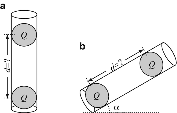
  Figure 3.30

• 3.4 Repulsion Forces: Two point charges, each with charge q = 10⁻⁹ C, are suspended by two strings, 0.2 m long, and connected to the same point as in Figure 3.31. If each charge has a mass of 10⁻⁴ kg, find the horizontal distance between the two charges under the assumption that α is small.

  

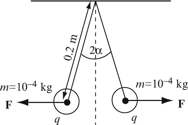
  Figure 3.31

• 3.5 Application: The Electrometer. An electrometer is a device that can measure electric field intensities or charge. One simple implementation is shown in Figure 3.31. Two very small conducting balls are suspended on thin conducting wires. To apply the charge, the test charge is placed at the point of contact of the two wires. The balls repel each other since half the charge is distributed on each ball.

  Suppose you need to design an instrument of this sort. Each wire is 0.2 m long and the mass of each ball is 10⁻⁴ kg. Assume each ball acquires half the measured charge and the balls are small enough to be considered as points:

  • (a) If the minimum distance measurable is 0.5 mm along the circumference of the circle the ball describes as it is deflected (arclength), what is the lowest amount of charge this instrument can measure?

  • (b) Can you also calculate the largest amount of charge measurable? Explain.

• 3.6 Force on Point Charge. Two positive point charges, each equal to Q [C], are located a distance d [m] apart. An electron, of charge e [C] and mass m [kg], is held in position on the centerline between them and at a distance x [m] from the line connecting the two charges as shown in Figure 3.32. The electron is now released:

  • (a) Calculate the acceleration the charge is experiencing (direction and magnitude). Where is the acceleration maximum?

  • (b) If there are no losses and no external forces, what is the path the electron describes?

  

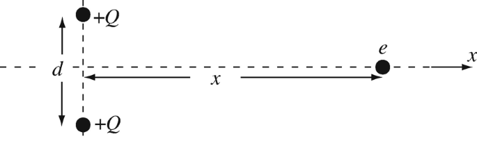
  Figure 3.32

• 3.7 Force on Point Charge. Two point charges are located at a distance d [m] apart. One charge is Q₁ = +q [C], the other is Q₂ = +2q [C], as in Figure 3.33. A third charge, +q [C], is placed somewhere on the line connecting the two charges:

  • (a) Assuming the third charge can only move on the line connecting Q₁ and Q₂, where will the charge move?

  • (b) From this stationary point, the charge is given a small vertical push (up or down) and allowed to move freely. Describe qualitatively the motion of the charge as it moves away from the two stationary charges.

  

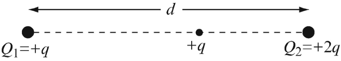
  Figure 3.33

• 3.8 Electric Field of Point Charges. Two point charges are located as in Figure 3.34:

  • (a) Sketch the electric field intensity of this arrangement using field lines.

  • (b) Find a point (on the axis) where the electric field intensity is zero.

  

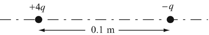
  Figure 3.34

• 3.9 Electric Field of Point Charges. Four point charges are arranged as shown in Figure 3.35 in free space:

  • (a) Find the electric field intensity at an arbitrary point in space.

  • (b) If Q₁ = Q₂ = Q and Q₃ = Q₄ = −Q show that the electric field intensity is perpendicular to the two dotted lines shown (at 45°).

  • (c) If Q₁ = Q₂ = Q₃ = Q₄ = Q show that the electric field intensity is parallel to the two dotted lines shown (at 45°).

  

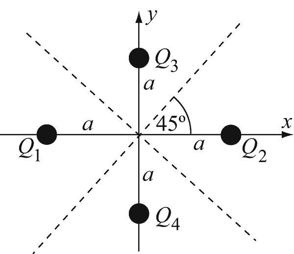
  Figure 3.35

• 3.10 The Quadrupole. Three point charges are located as shown in Figure 3.36. The outer charges equal q [C] and the center charge equals −2q [C]. This arrangement is called a linear quadrupole because it consists of two dipoles on a line:

  • (a) Find the electric field intensity at an arbitrary point P a distance R [m] from the negative charge.

  • (b) Use the binomial expansion to obtain an approximate solution for the electric field intensity at P for R ≫ d. Retain the first three terms in the expansion and then neglect those terms in the approximation that can be justifiably neglected.

  • (c) Sketch the field lines of the quadrupole and compare with those of the dipole in Section 3.4.1.3 (Figure 3.12).

  

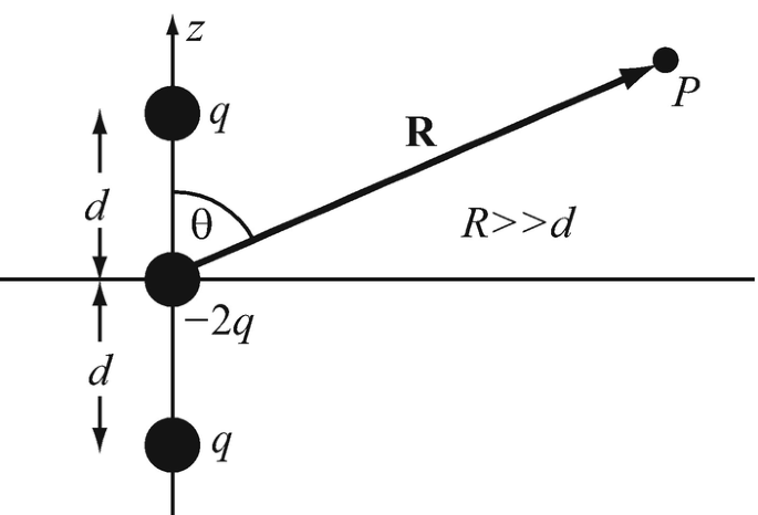
  Figure 3.36

• 3.11 Electric Field and Forces Due to Point Charges. Two positive point charges each equal to Q [C] and two negative charges each equal to –Q [C] are placed at the corners of the base of a pyramid as shown in Figure 3.37. The base is a square a × a m² in dimensions. A 5th point charge –Q [C] is placed at the pinnacle of the pyramid. If all edges of the pyramid equal to a [m], calculate:

  • (a) The electric field intensity at the pinnacle of the pyramid.

  • (b) The electric field intensity at the center of the base of the pyramid.

  • (c) The force on the negative charge at the pinnacle.

  

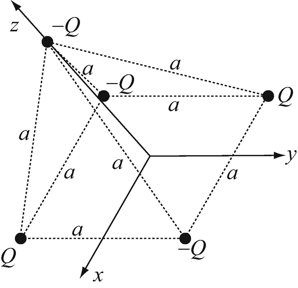
  Figure 3.37

• 3.12 Application: Electrostatic Levitation—Repulsion Mode. The repulsion force between charges can be used to levitate bodies by ensuring the repulsion force is equal to the weight of the levitated body. Suppose four small plastic balls are placed at the corners of a rigid square, a [m] on the side, and charged each to +100 nC. Four identically charged balls are embedded into a fixed plane, with the distance between the balls also a [m]. Assume the levitation h is small compared to the length a (h ≪ a), and the weight of the frame is negligible:

  • (a) If the movable frame is placed with its charges exactly above the four stationary charges and if the mass of each ball is 10⁻⁴ kg, calculate the elevation at which the movable frame levitates.

  • (b) If the movable frame is allowed to rotate but not to translate, what is the rest position of the charges? Do not calculate the position; just describe it.

  • (c) Suppose you push the movable frame downward slightly from the position in (b) and release it. What happens to the frame?

  • (d) Suppose you move the frame downward until the movable charges are in the same plane as the stationary charges. Disregarding mechanical questions of how this can be done, what happens to the frame now?

  • (e) If you continue pushing until the frame is below the plane, what will be the stationary position of the frame?

• 3.13 Application: Electrostatic Levitation—Attraction Mode. The situation in Problem 3.12 is given again, but the stationary charges are positive and the movable charges are negative and of the same magnitude:

  • (a) Find the position at which the frame is stationary (below the plane). Assume the distance h [m] between the frames is small compared to the frame’s size (h ≪ a) and the frame is free to rotate in its plane.

  • (b) If the frame is pushed either downward or upward slightly, what happens?

  • (c) Compare with Problem 3.12. Which arrangement would you choose?

• 3.14 Force on Charge in an Electric Field. Two stationary point charges, each equal in magnitude to q [C], are located a distance d [m] apart. A third point charge is placed somewhere on the line separating the two charges and is allowed to move. The charge is free to move in any direction:

  • (a) If the stationary charges are positive and the moving charge is positive, it will move to the midpoint between the two stationary charges. Is this a stable position? If not, where will the charge eventually end up if its position is disturbed?

  • (b) What is the answer to (a) if the stationary charges are positive but the moving charge is negative?

  • (c) What is the answer to (a) and (b) if the stationary charges are negative?

• 3.15 Application: Accumulation of Charge. One of the common mechanisms for charge to accumulate in clouds is through friction due to raindrops. In the process, each drop acquires a positive charge, while the cloud tends to become more negative. Suppose each raindrop is 2 mm in diameter and each acquires the charge of one proton. If it rains at a rate of 10 mm/h, what is the rate of transfer of charge to earth per unit area?

• 3.16 Electric Field of Point Charges. Three point charges are placed at the vertices of an equilateral triangle with sides of length L [m]:

  • (a) Each charge is equal to q [C]. Find the points in space at which the electric field intensity is zero.

  • (b) Two charges are equal to q [C], the third to 2q [C]. Show that the electric field intensity is zero only at infinity.

  Hint: To find the answers you will need to solve a transcendental equation. Use a graphical method to find the roots of the equation.

• 3.17 Application: Millikan’s Experiment—Determination of the Charge of Electrons. A very small oil drop has a mass of 1 μg. The oil drop is placed between two plates as shown in Figure 3.38. A uniform electric field intensity E is applied between the two plates, pointing down:

  • (a) What is the electric field intensity that will keep the drop suspended without moving up or down if the drop contains one free electron?

  • (b) What is the next (lower) value of field possible and what is the charge on the drop?

    

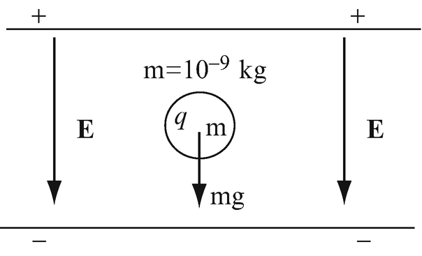
    Figure 3.38

• 3.18 Force in a Uniform Field. A uniform electric field intensity of 1,000 N/C is directed upwards. A very small plastic ball of mass 10⁻⁴ kg is charged with a charge such that the ball is suspended motionless in the field:

  • (a) Calculate the charge on the ball assuming a point charge. Find the magnitude and sign of the charge.

  • (b) If the charge is doubled and the ball allowed to move starting from rest, find the acceleration of the ball.

  • (c) If the ball starts from rest, in a frictionless environment, find the time it takes the ball to reach a speed equal to half the speed of light under the condition given in (b).

• 3.19 Application: Electrostatic Air Cleaner. An air cleaner is made as two parallel plates with an electric field intensity of 10 kN/C between the plates as shown in Figure 3.39. The cleaner is installed in a vertical chimney to collect dust particles as these rise through the chimney. Assume the air and particles are pushed upwards at a velocity of 10 m/sec and that particles have been charged with an electric charge of one electron each before entering the chamber. Calculate the mass of the heaviest particle that is guaranteed not to escape the cleaner chamber.

  

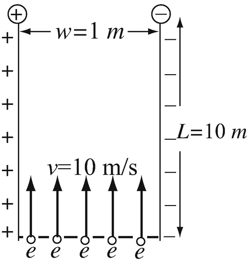
  Figure 3.39

3.1.2 Line Charge Densities

• 3.20 Field Due to Line Charge Density. A short line of length L [m] is charged with a line charge density ρ_l [C/m] (see Figure 3.40). Calculate the electric field intensity at the four points shown in Figure 3.40.

  

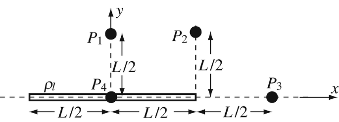
  Figure 3.40

• 3.21 Field Due to a Charged Ring. A thin ring of radius a [m] is charged so that a uniform line charge density of ρ_l [C/m] exists on the ring:

  • (a) Calculate the electric field intensity at a height h [m] above the center of the ring, on its axis.

  • (b) Show that at very large distances (h ≫ a), the electric field intensity is that of a point charge equal to the total charge on the ring.

• 3.22 Force on Line Charge Density. A charged line 1 m long is charged with a line charge density of 1 nC/m. A point charge is placed 10 mm away from its center. Calculate the force acting on the point charge if its charge equals 10 nC.

• 3.23 Electrostatic Forces. Two thin segments, each 1 m long, are charged, one with line charge density of 10 nC/m and the other with −10 nC/m and are placed a distance 10 mm apart, parallel to each other. Calculate the total force one segment exerts on the other.

• 3.24 Force Between Two Short Charged Segments. Two charged lines are colinear as shown in Figure 3.41. The total charge on line 1 is Q₁ [C]; the total charge on line 2 is Q₂ [C]. On each line the charge is uniformly distributed over the length of the line. Given the lengths of the lines (L₁ [m] and L₂ [m]) and the distance between them as a [m], calculate the force one line exerts on the other if both are in free space.

  

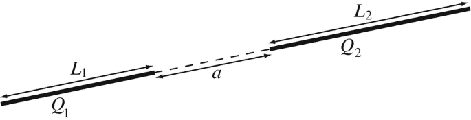
  Figure 3.41

• 3.25 Force Between Charged Lines. A very long thin conductor is charged with a uniform line charge density ρ_l [C/m]. A second, short conductor, placed vertically on the same plane as the long conductor has length b [m] and a uniform line charge density −ρ_l [C/m] (see Figure 3.42). Calculate the force the short line exerts on the longer line. The conductors are in free space.

  

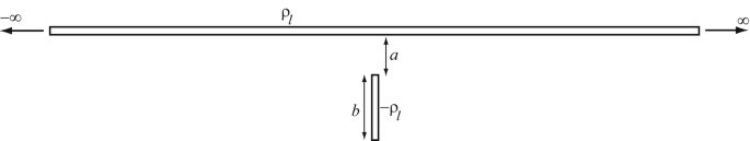
  Figure 3.42

3.1.3 Surface Charge Densities

• 3.26 Electric Field Due to Surface Charge Density. A disk of radius a [m] is charged with a uniform surface charge density ρ_s [C/m²] (see Figure 3.43).

  • (a) Calculate the electric field intensity at a distance h [m] from the center of the disk on the axis.

  • (b) Plot the magnitude of the electric field intensity for all values of h from h = −5a to h = 5a for a = 10 mm, ρ_s = 2 nC/m².

  • (c) What is the maximum electric field intensity and at what height does it occur?

  • (d) What is the electric field intensity in (a) if a → ∞?

  

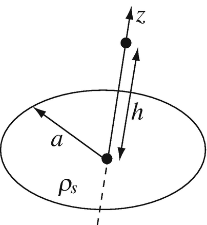
  Figure 3.43

• 3.27 Electric Field Due to Surface Charge Density. A disk of radius a [m] is charged with a nonuniform charge density ρ_s = ρ₀r² [C/m²], where r [m] is the distance from the center of the disk.

  • (a) Calculate the electric field intensity at a distance h [m] from the center of the disk, on the axis (see Figure 3.43).

  • (b) Plot the magnitude of the electric field intensity for all values of h from h = −5a to h = 5a for a = 10 mm, ρ₀ = 2 × 10⁻⁹.

• 3.28 Electric Field of Infinite Surface. Calculate the electric field intensity in free space at a distance d [m] above an infinite plane charged with a uniform surface charge density ρ_s [C/m²]. Show that the electric field intensity is independent of d and is perpendicular to the plane.

• 3.29 Charged Infinite Plate with a Hole. A thin infinite plate is charged with a uniform surface charge density ρ_s [C/m²]. A disk of radius a [m] is removed so that a hole of radius a [m] is left at the center of the plate (no charge on the surface occupied by the hole). Calculate the electric field intensity at a height a [m] above the center of the hole in free space.

• 3.30 Electric Force Due to Hollow, Charged Cylindrical Surface. A very thin-walled cylindrical tube of length L [m] and radius a [m] has a surface charge density ρ_s [C/m²] uniformly distributed as shown in Figure 3.44. A point charge Q [C] is placed at point P on the axis of the tube. Calculate the force on the charge Q (magnitude and direction). The tube is drawn in axial cross section.

  

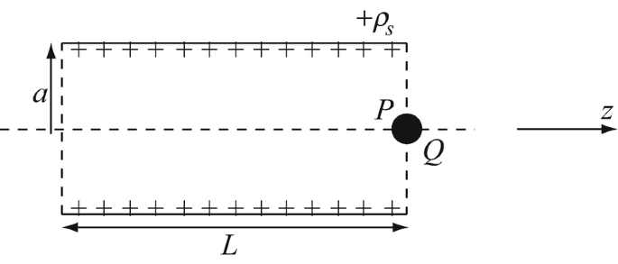
  Figure 3.44

3.1.4 Volume Charge Densities

• 3.31 Field Due to Volume Charge Density. A short plastic cylinder of length L [m] and diameter L/2 [m] has a uniform volume charge density ρ_v [C/m³] uniformly distributed throughout its volume.

  • (a) Calculate the electric field intensity at all points on the z-axis (Figure 3.45).

  • (b) Find the location of maximum field on the z-axis.

  

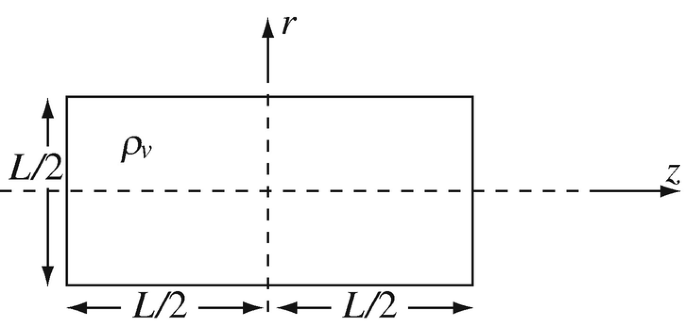
  Figure 3.45

• 3.32 Electric Field of the Electron. The structure of the electron is not defined (i.e., its dimensions cannot be identified with certainty). Its charge, however, is considered to be a point charge. Consider the following:

  • (a) Suppose the electron is a point charge equal to e = −1.602 × 10⁻¹⁹ C. Calculate the electric field intensity it produces everywhere in space.

  • (b) Suppose now that the charge of the electron is distributed uniformly over a spherical volume of radius R₀ = 2 × 10⁻¹³ m. Calculate the electric field intensity everywhere in space outside the electron (that is, for R > R₀). Show that the result is the same as in (a). Hint: To simplify solution, assume that the sphere is made of a stack of disks of varying radii and differential thickness dz′ and calculate the electric field intensity on the axis of the disk (see, for example, Problem 3.26).

• 3.33 Electric Field of Small Volume Charge Density. A small sphere of radius a [m] has a nonuniform volume charge density given as ρ_v = ρ₀R(a − R)/a [C/m³] where R [m] is the distance from the center of the sphere. Find the electric field intensity at a very large distance R ≫ a. What are the assumptions you must make?

3.1.5 The Electric Flux Density

• 3.34 Electric Flux Density Due to Point Charges. Two point charges are separated a distance d [m] apart. Each charge is 10 nC and both are positive:

  • (a) Calculate the force between the two charges.

  • (b) Both charges, while still at the same distance, are immersed in distilled water (ε = 81ε₀). What is the force between the charges in water? Explain the difference.

  • (c) What can you say about the electric field intensity and electric flux density in air and water?

• 3.35 Electric Flux Density in Dielectrics. A point charge is located in free space. The charge is surrounded by a spherical dielectric shell, with inner diameter d₁ [m], outer diameter d₂ [m], and permittivity ε [F/m]. Calculate:

  • (a) The electric flux density everywhere in space.

  • (b) The electric field intensity everywhere in space.

  • (c) The total electric flux passing through the outer surface of the dielectric shell.

  • (d) The total flux passing through the inner surface of the dielectric.

  • (e) The total flux through a spherical surface of radius R > d₂/2 in air.

  • (f) What is your conclusion from the results in (c), (d), and (e)?