Antennas and Electromagnetic Radiation

Ida, Nathan

doi:10.1007/978-3-030-15557-5_18

Nathan Ida²

2518 Accesses
1 Citations

Abstract

After discussing wave propagation, it is time we go back and discuss the sources of the waves. Recall that our whole discussion of waves was based on the solution to the source-free wave equation. Starting with Chapter 11, we assumed that a wave was generated in some fashion but did not concern ourselves too much with how the wave was generated. Occasionally, the term “source” or “antenna” was mentioned but only to indicate that the wave must have a source.

Is it a fact—or have I dreamt it—that, by means of electricity, the world of matter has become a great nerve, vibrating thousands of miles in a breathless point of time? Rather, the round globe is a vast head, a brain, instinct with intelligence!

—Nathaniel Hawthorne (1804–1864),

Novelist

This is a preview of subscription content, log in via an institution to check access.

Access this chapter

Log in via an institution

eBook: USD 16.99; Price excludes VAT (USA)

Softcover Book: USD 89.99; Price excludes VAT (USA)

Hardcover Book: USD 109.99; Price excludes VAT (USA)

Tax calculation will be finalised at checkout

Purchases are for personal use only

Institutional subscriptions

Notes

1.
Radar has a long and interesting history. Although it appeared as a military instrument around the beginning of WWII (a radar installation in Hawaii detected the attack planes heading for Pearl Harbor, but the warning was ignored), its development started much earlier. The first reported radar experiment goes back to 1904 when Christian Hulsmeyer used waves from a spark gap (at a wavelength of about 0.5 m) to show azimuthal location capabilities at 3 km, for which he received the first radar patent. He called his device a “telemobiloscope.” After that, many more experiments were performed, including experiments by Guglielmo Marconi (1874–1937), and as early as 1925, primitive forms of radar were used for remote sensing of the ionosphere. The development of radar for detection and tracking of aircraft started in 1935 in Britain, and after the development of the magnetron and klystron (both are microwave tubes used for generation of waves at high frequencies), the radar became a reality at the beginning of WWII. From then on, radar became a household name and, today, it is used in many areas from storm prediction and detection to mapping of planets to looking for dinosaurs’ bones to collision avoidance.
2.
Although parabolic antennas are rather new, it is worth mentioning that in 1888, Heinrich Hertz used a parabolic reflector to focus electromagnetic waves. In his experiments, he used a spark gap which radiated at a wavelength of about 0.6 m. He designed a wooden frame, about 2 m by 1.2 m, and coated it with zinc to obtain the first parabolic reflector.

Author information

Authors and Affiliations

Department of Electrical Engineering, University of Akron, Akron, OH, USA
Nathan Ida

Authors

Nathan Ida
View author publications
You can also search for this author in PubMed Google Scholar

Corresponding author

Correspondence to Nathan Ida .

Problems

18.1.1 Hertzian Dipole

18.1
Near and Far Fields of Antennas. In preparation for a propagation experiment, a researcher places a field measuring instrument (an antenna) at a distance of 150 m from a transmitting antenna, which operates at 30 GHz. Is the instrument in the near or the far field of the transmitting antenna?
18.2
The Hertzian Dipole. A short dipole antenna is 0.02 λ long and carries a current of 2 A at 150 MHz. Calculate (in free space):
1. (a)
  The electric and magnetic field intensities in the near field.
2. (b)
  The electric and magnetic field intensities in the far field.
3. (c)
  The radiation resistance and radiated power of the antenna.
4. (d)
  Maximum range in the direction of maximum power density if the time-averaged power density required for reception is 10⁻¹⁰ W/m².
18.3
Radiated Power. An antenna produces an electric field intensity in the far field:
$$ \mathbf{E}=\hat{\boldsymbol{\uptheta}}\frac{jV_0}{R}{\mathrm{e}}^{-j{\beta}_0R}\sin \theta \kern1em \left[\frac{\mathrm{V}}{\mathrm{m}}\right] $$
where β₀ [rad/m] is the phase constant in free space, R [m] is the distance from the source (antenna), and θ is the angle with respect to the vertical (z) axis. Calculate:
1. (a)
  The radiated time-averaged power density.
2. (b)
  The total time-averaged power radiated by the antenna.
18.4
Application: The Dipole Antenna. A dipole antenna is 1 m long and is fed with a current of amplitude 2 A. Find the radiated power of the antenna in free space:
1. (a)
  At 540 kHz (lowest AM band frequency).
2. (b)
  At 1.6 MHz (highest AM band frequency).
3. (c)
  To what do you attribute the difference between the radiated powers in (a) and (b)?
18.5
Power Line as Antenna. Calculate the power radiated by one conductor of a single phase high voltage power line one km long carrying a current of 250 A at 60 Hz. Neglect the effect of the ground and the proximity of other lines. Treat air as free space.

18.1.2 Magnetic Dipole

18.6
Application: Magnetic Dipole (Loop) Antenna. A transmitter uses a Hertzian dipole, 0.02λ long. Because of changes in design, it becomes necessary to replace the Hertzian dipole by an equivalent magnetic dipole (loop) antenna, keeping the current in the loop the same as the current in the dipole:
1. (a)
  What is the radius of the loop that will produce the same fields in the far field?
2. (b)
  What is the orientation of the loop with respect to the Hertzian dipole?
18.7
The Small-Loop Antenna. A magnetic dipole (loop) antenna is made of 10 turns, closely wound. The turns are of radius a [m]. A current I₀cosωt [A] flows in the antenna:
1. (a)
  Find the radiated power of the antenna in free space.
2. (b)
  Find an expression for the radiation resistance of the antenna in free space.
3. (c)
  Extend the expressions in (a) and (b) to an n-turn loop antenna.

18.1.3 Linear Antennas of Arbitrary Length

18.8
Application: The Short Dipole Antenna. A short dipole is a dipole that is too long to be considered a Hertzian dipole but too short to be an arbitrarily long antenna. This usually means an antenna between λ/50 and λ/10 in. length. Given: In the short dipole, the current is linear that is, I(z′) = I₀(1 − (2/l)∣z′∣) [A], where l = λ/20 is the total length of the dipole and I₀ [A] is a constant amplitude. Calculate:
1. (a)
  The far-field electric field intensity, magnetic field intensity, and power density.
2. (b)
  The radiation resistance and radiation pattern of the dipole.
18.9
Arbitrary-Length Dipole. A communication system uses a dipole antenna for transmission. Calculate:
1. (a)
  The maximum power density received 5 km away given the following: I₀ = 2 A, dipole length is d = 80 cm, wavelength is λ = 1 m, propagation is in free space.
2. (b)
  The radiated power of the antenna.
3. (c)
  The radiation resistance of the antenna.
4. (d)
  Maximum directivity of the antenna.
18.10
Radiation Efficiency. Find the radiation efficiencies of the following antennas. They are made of round copper wire of radius a = 0.4 mm and conductivity σ = 5.7×10⁷ S/m. Permeability of copper is the same as that of free space.
1. (a)
  A dipole of length 2 m operating at 1 MHz.
2. (b)
  A dipole of length 1.5 m operating at 100 MHz.

18.1.4 The Half-Wave Dipole Antenna

18.11
Application: λ/2 Dipole. A half-wavelength antenna is made of copper wire with conductivity σ = 5.7 × 10⁷ S/m and permeability μ₀ = 4π × 10⁻⁷ H/m. The antenna is 3 mm thick and 1.5 m long:
1. (a)
  Calculate the impedance of the antenna and its efficiency when radiating in free space.
2. (b)
  In an attempt to reduce the impedance and increase efficiency, the antenna is made of a copper tube, 12 mm in diameter. What is the efficiency of the antenna? Assume current flows entirely within one skin depth, on the surface of the wire.
18.12
Application: Simple Dipole Antenna. Suppose you need a good antenna in a hurry for a transmitter operating at 27 MHz. A friend suggests the following: Take a two-wire cable, with characteristic impedance of 72 Ω. Split the cable for a length of 2.77 m. Bend the two wires so that they are perpendicular to the cable and on a line as shown in Figure 18.43. To support it, the friend suggests tacking it onto a nonconducting wall:
1. (a)
  What kind of antenna is this antenna?
2. (b)
  If the conductor is 1 mm thick and made of copper (σ = 5.7 × 10⁷ S/m, μ = 4π × 10⁻⁷ H/m), what is the efficiency of the antenna?
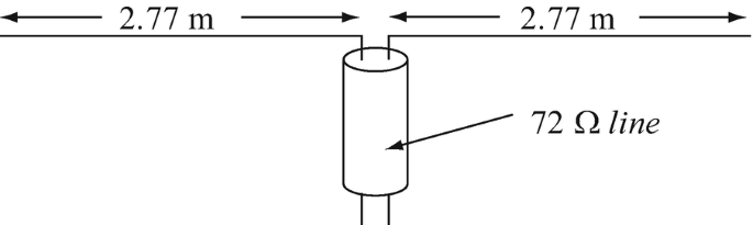
  Figure 18.43
18.13
Radiated Power of λ/2 Dipole. A half-wavelength antenna is given. The maximum magnetic field intensity of the antenna at a distance of 120 m is measured and found to be equal to 1 mA/m (peak value). Radiation is at a wavelength of 1 m.
1. (a)
  Assuming free space, calculate the radiated power of the antenna.
2. (b)
  Calculate the radiated power of the antenna if the space also has a conductivity of 10⁻⁶ S/m.
18.14
Properties of λ/2 Dipole. A half-wavelength dipole is driven at 100 MHz with a current of 10 A (peak). The antenna may be assumed to be at ground level and perpendicular to the ground. Neglect the effect of the ground. An airplane receives transmission from the antenna when it is at 100 km horizontal distance from the antenna and at 10 km elevation above ground. Calculate assuming air has properties of free space:
1. (a)
  The time-averaged power density at the airplane.
2. (b)
  The antenna gain in the direction of the airplane.
18.15
Fields of λ/2 Dipole. A half wavelength dipole is directed vertically (z-axis) and radiates a time averaged power density of 28 W in free space at a frequency of 275 MHz. Find the amplitudes of the electric and magnetic field intensities at a distance R = 100 m from the center of the antenna, at θ = 90° and ϕ = 30°.

18.1.5 Various Length Dipole Antennas

18.16
Radiation Resistance and Standing Wave Ratio. An antenna is connected to a 50 Ω transmission line. The antenna radiates in free space. Calculate the standing wave ratio on the transmission line if:
1. (a)
  The antenna is a half-wavelength dipole with zero internal resistance.
2. (b)
  The antenna is a half-wavelength dipole with internal resistance of 1.2 Ω.
3. (c)
  The antenna is a Hertzian dipole, λ/50 long and has no internal resistance.
18.17
Various Length Dipoles. Find and plot the current distribution along a dipole antenna of the following length:
1. (a)
  λ/2.
2. (b)
  λ.
3. (c)
  3λ/2.
4. (d)
  3λ/4.
5. (e)
  2λ.
6. (f)
  5λ/4.
18.18
Various Length Dipoles. Find and plot the normalized E-plane field radiation pattern of the following dipole antenna lengths:
1. (a)
  0.75λ.
2. (b)
  1λ.
3. (c)
  1.5λ.
4. (d)
  2λ.
5. (e)
  2.5λ.
18.19
Radiation Resistance, Directivity, and Radiated Power. Calculate the radiation resistance, directivity, and radiated power (in free space) of a 3λ/2 dipole carrying a peak current of 0.2 A.
18.20
Radiation Resistance, Directivity, and Radiated Power
1. (a)
  Estimate the radiation resistance of a 1.25λ dipole in free space using Table 18.2 and Figure 18.15.
2. (b)
  Calculate the exact radiation resistance of the 1.25λ dipole in free space.
3. (c)
  Calculate the directivity of the 1.25λ dipole using the estimate in (a) and by exact calculation.

18.1.6 The Monopole Antenna

18.21
Application: λ/2 Monopole. A half-wavelength monopole antenna is used for FM transmission at 100 MHz. The antenna is placed vertically above a conducting surface in free space. Find:
1. (a)
  The antenna length.
2. (b)
  The radiation resistance of the monopole.
3. (c)
  The radiated power of the monopole for a current of amplitude I₀.
4. (d)
  The directivity of the monopole at θ = π/2.
18.22
Application: Short Monopole. A short monopole is used in a mobile telephone. The limitation is that a telephone of this type should not transmit more than 0.6 W. If the telephone transmits at 76 MHz and the antenna length is 0.1 m:
1. (a)
  Calculate the required current in the antenna. Assume a perfect conductor for the antenna.
2. (b)
  What is the maximum range of the telephone if the amplitude of the electric field intensity at the receiving antenna should be no lower than 10 mV/m?
18.23
Monopole Antennas: Efficiency. Two quarter-wavelength monopoles are used at the same frequency. Both are made of copper, with conductivity 5.7 × 10⁷ S/m. Both transmit at 1 GHz. One is 1 mm thick, the second is 10 mm thick.
1. (a)
  Which antenna has higher efficiency?
2. (b)
  What are the efficiencies of the two antennas if both transmit in free space?
3. (c)
  Calculate the ratio between the (power) gains of the two antennas.
18.24
Application: The Monopole Antenna. A short monopole antenna is used at 1 MHz for AM transmission. The antenna is 0.5 m long and placed vertically above a conducting surface in air (free space). Find:
1. (a)
  The radiation resistance of the monopole.
2. (b)
  The radiated power of the monopole for a given current.
3. (c)
  The maximum directivity of the monopole.
18.25
Application: λ/4 Monopole. A quarter-wavelength monopole antenna is used at 100 MHz. The antenna is placed vertically above a conducting surface in air (free space). Find:
1. (a)
  The physical length of the antenna.
2. (b)
  The radiation resistance of the monopole.
3. (c)
  The radiated power of the monopole for a given current.
4. (d)
  The maximum directivity of the monopole.

18.1.7 Two-Element Image Antennas

18.26
Two-Element Array. A Hertzian dipole antenna of length d is placed horizontally above a perfectly conducting ground at a height h [m]. Assuming a current in the antenna of amplitude I₀ [A]:
1. (a)
  Find the electric and magnetic fields in the far field of the antenna.
2. (b)
  Find the radiation pattern of the antenna.
18.27
Two-Element Array. A wire antenna is placed perpendicularly above the ground. The wire is 3 m long and is used in conjunction with a transmitter which operates at 100 MHz:
1. (a)
  Find the field radiation pattern of the antenna.
2. (b)
  For a current I = 1 A, find the radiated power of the antenna in free space.
3. (c)
  Suppose the wire length is adjusted so that it is exactly 1.5 wavelengths. What are now the field radiation pattern and radiated power? Compare with (a) and (b).
18.28
Two-Element Arrays. Two half-wavelength dipole antennas are placed a distance d apart, parallel to each other. Calculate and plot the field radiation patterns for:
1. (a)
  d = 0, φ = 0° (zero separation, in phase)
2. (b)
  d = 0.5λ, φ = 0.
3. (c)
  d = 0.5λ, φ = π [rad].
4. (d)
  d = 0.5λ, φ = π/2 [rad].
5. (e)
  d = 0.5λ, φ = π/4 [rad].
6. (f)
  d = 1λ, φ = 0.
7. (g)
  d = 1λ, φ = π [rad].
8. (h)
  d = 1λ, φ = π/2 [rad].
9. (i)
  d = 1λ, φ = π/4 [rad].
10. (j)
  d = 1.5λ, φ = 0.
11. (k)
  d = 1.5λ, φ = π [rad].
12. (l)
  d = 1.5λ, φ = π/2 [rad].
13. (m)
  d = 1.5λ, φ = π/4 [rad].
18.29
Two-Element Array. Two half-wavelength antennas are spaced 10 wavelengths apart:
1. (a)
  If the two antennas are driven in phase, find the radiation pattern of the array.
2. (b)
  If the two antennas are driven with a phase difference of π/2 [rad], find the field radiation pattern of the array.
3. (c)
  Describe how the pattern changes as the antennas are moved further apart.
18.30
Magnetic and Hertzian Dipoles. An antenna is built as a combination of a Hertzian dipole of length 0.05λ and a small magnetic dipole (loop) loop of diameter 0.025λ. The dipole is placed at the center of the loop so that the plane of the loop is perpendicular to the dipole, at its center (see Figure 18.44). The two antennas are driven at 100 MHz with a current of magnitude I₀ = 0.1 A. For convenience place the loop on the x–y plane at z = 0 and the dipole on the z axis, symmetrically about the x–y plane in free space:
1. (a)
  Find the electric and magnetic intensities in the far field if the currents in the antennas are in phase.
2. (b)
  Find the electric and magnetic field intensities in the far field if the current in the loop lags behind the current in the dipole by 180°.
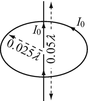
  Figure 18.44
18.31
Magnetic and Hertzian Dipoles. In Problem 18.30 assume the currents in the dipole and in the loop are I₁ and I₂, but they are in phase:
1. (a)
  Find the polarization of the wave in the far field.
2. (b)
  Suppose the current in the magnetic dipole (loop) and in the dipole are individually adjustable, but their phase is fixed. What are the types of polarization that may be achieved?
3. (c)
  Suppose the currents in the loop and Hertzian dipole remain constant in magnitude, but their phases may be changed individually. What are the types of polarization achievable? See Section 12.8 for the concept of polarization.

18.1.8 The n-Element Linear Array

18.32
Application: Linear Antenna Array. An array antenna is made of six identical elements, each a half-wavelength dipole, and is fed with identical currents, all in phase. Spacing of the elements is one-half wavelength. Assume the antennas are placed on the x axis and are parallel to the z axis. Find:
1. (a)
  The normalized array field radiation pattern.
2. (b)
  The normalized array power radiation pattern.
3. (c)
  The direction of maximum radiation.
4. (d)
  The directions of the sidelobes.
18.33
Linear Arrays. An antenna array is made of n half-wavelength dipoles, parallel to each other, all placed on the x-axis and directed in the z direction. Find and plot the normalized field array antenna radiation patterns for the following number of elements N, spacing h [m], phase constant β = π [rad/m], and progressive phase angle φ [rad] of each consecutive element with respect to the previous element starting with zero phase angle for the first element in the array. Plot the patterns for 0 ≤ θ ≤ π and ϕ = π/4:
1. (a)
  N = 5, h = 0.6 m, φ = −0.6π [rad].
2. (b)
  N = 6, h = 0.6 m, φ = −π [rad].
3. (c)
  N = 10, h = 0.7 m, φ = −0.75π [rad].
4. (d)
  N = 5, h = 0.7 m, φ = π [rad].
18.34
Five-Element Array. An antenna array is made of five Hertzian dipoles, spaced λ/4 apart, and driven in phase. The dipoles are parallel to each other. Using the notation in Figure 18.33:
1. (a)
  Find the array radiation pattern of the antenna.
2. (b)
  What is the direction of maximum power?
18.35
Application: 5 Element Array. A three-element array as shown in Figure 18.45 carries currents I₁ = I₃ = I₀ [A] and I₂ = 2I₀ [A]. Calculate and plot the antenna radiation pattern, with all elements in phase:
1. (a)
  In the plane of the elements.
2. (b)
  In the plane perpendicular to the elements.
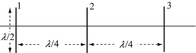
  Figure 18.45
18.36
Linear Array of Monopoles. An array is made of n monopoles, all perpendicular to the ground and separated one-half wavelength from each other. The monopoles are 0.25λ long and are all in phase. For orientation purposes place the monopoles on the x-axis and calculate:
1. (a)
  The array field radiation pattern and plot it in a plane that includes the monopoles and in a plane perpendicular to the monopoles.
2. (b)
  The electric and magnetic field intensities at a general point in space for a given current. All monopoles carry identical currents.
18.37
Linear Magnetic Dipole (Loop) Array. An antenna array is made of n magnetic dipoles (loops), all lying flat on a surface in a line, separated a distance 2d apart where d = 0.02λ is the diameter of the loop. For orientation purposes place the loops on the x-axis.
1. (a)
  Calculate the electric and magnetic field intensities in the far field of the array, given a current I [A] in each loop and a phase difference φ between each two consecutive loops. Assume free space propagation.
2. (b)
  Calculate the array factor and the normalized array factor if all elements are in phase.
3. (c)
  Explain the relation between the result obtained here and that for a linear array of Hertzian dipoles.
18.38
Application: Co-Linear Array. Five (5) half-wavelength dipole antennas are stacked on a line as in Figure 18.46 to form a co-linear array. The centers of each two dipoles are a distance λ apart and the antennas are in free space. The currents in all elements have the same magnitude and the same phase. Use the system of coordinates shown and write the expression in terms of the radial distance R from the center of the array and calculate:
1. (a)
  The electric and magnetic field intensity of the array in the far field.
2. (b)
  The time-averaged power density of the array.
3. (c)
  Plot the E-plane field radiation pattern of the array.
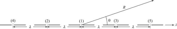
  Figure 18.46
18.39
Application: Superposition of Linear Arrays. A Hertzian dipole is placed at a distance λ/2 in front of a corner conductor to form a reflector antenna as shown in Figure 18.47. The dipole is parallel to the corner and symmetrically placed with respect to the conducting surfaces, with its current in the negative z direction. The corner conductor may be assumed to be very large. The dipole operates at a wavelength λ and transmits in free space. Assume there are no losses in the system (i.e., the dipole and the corner conductor are made of perfect conductors). For orientation purposes, use the system of coordinates shown with the origin at the corner. Calculate:
1. (a)
  The array factor of the reflector antenna.
2. (b)
  The time-averaged power density of the reflector antenna.
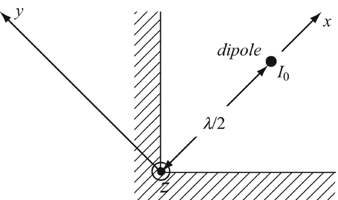
  Figure 18.47
18.40
Application: Superposition of Linear Arrays. A seven (7)-element linear array is made of half-wavelength dipoles, all parallel, and the distance between each two elements is h = λ/4. Taking the middle of the array as reference, calculate the time-averaged power density of the array in the far field given that the magnitude of the current in all elements is I₀ [A] but their directions alternate (see Figure 18.48. You may assume the antennas are oriented in the z direction and placed on the x axis, symmetrically about the origin in free space.
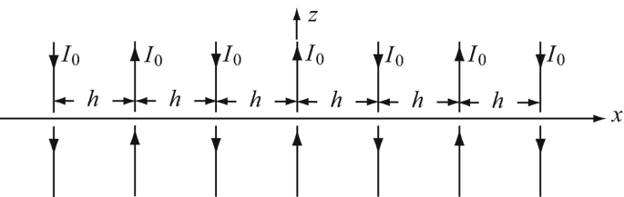
Figure 18.48
18.41
Nonuniform Linear Array. A 6 element array is made of Hertzian dipoles, each Δl = 2 cm long with their centers lying on the x axis in free space. The spacings are shown in Figure 18.49. The amplitude of each element is I₀ = 0.1 A. The array radiates at 432 MHz and all elements are in phase.
1. (a)
  Find the time averaged power density at the center of the main beam at a distance of 250 m from the center of the array.
2. (b)
  Calculate the beamwidth of the main beam.
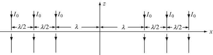
  Figure 18.49

18.1.9 Reciprocity and Receiving Antennas

18.42
Effective Area of a Monopole. The receiving antenna in an AM car radio is a 1 m long monopole, vertical above the body of the car. AM reception is between 520 kHz and 1.6 MHz. Calculate the effective area of the antenna at the two extremes of the frequency range, assuming properties of free space.
18.43
Application: Circular Magnetic Dipole (Loop) Receiving Antenna. A small circular loop of radius a [m] is used as a receiving antenna. The antenna is placed at a distance R [m] in the field of an isotropic antenna which radiates P [W] at a frequency f [Hz] in free space:
1. (a)
  What is the maximum power received by the loop antenna?
2. (b)
  What is the maximum peak current in the loop antenna?
18.44
Application: Receive–Transmit System. Two units communicate with each other at 120 MHz and 10 W, in free space. Unit A uses a half-wavelength dipole antenna placed as shown in Figure 18.50. Unit B uses a 1/100 wavelength long dipole antenna and is 10 km from the transmitting antenna as shown:
1. (a)
  Find the current in antenna B when unit A transmits.
2. (b)
  Find the current in antenna A when unit B transmits.
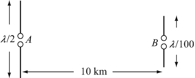
  Figure 18.50
18.45
Application: Receive–Transmit System. To evaluate the properties of an antenna, two identical antennas are used in a receive–transmit system. The two antennas are placed a distance d = 10 km apart in free space and one antenna transmits 10 W at 300 MHz. The second antenna receives 10 μW. The two antennas are adjusted so that the direction of maximum directivity coincides with the line connecting them. Calculate:
1. (a)
  The maximum directivity of the antenna.
2. (b)
  The maximum effective area of the antenna.
18.46
Application: Send–Receive System. A half-wavelength dipole antenna is placed vertically (to the surface of the earth) and transmits 1 W (time-averaged power) at a wavelength of 3 m. A second, identical antenna, also placed vertically, is on top of a mountain 1 km high and 1 km away (horizontally) from the first antenna as in Figure 18.51. Neglect all effects due to the earth and assume properties of free space for air:
1. (a)
  Calculate the current the receiving antenna supplies to the receiver assuming both antennas are matched.
2. (b)
  In an attempt to increase this current, both antennas are adjusted by tilting them from the vertical direction. How must they be tilted (sketch or give accurate description) and what is the maximum current obtainable by doing so?
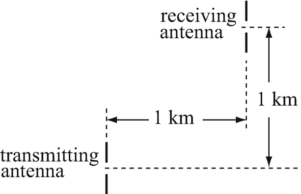
  Figure 18.51

18.1.10 Radar

18.47
Application: Radar Cross Section. A radar is used for navigational purposes. A fixed radar station transmits at 3 GHz and 100 kW. If the smallest ocean-going ship has a radar cross section of 200 m² and the radar antenna gain is 15 dB, find the effective range of the radar if detection requires a minimum of 1 nW/m² at the radar antenna. Neglect losses in the antenna and assume free space properties for air.
18.48
Application: λ/2 antenna in a Radar. A half wavelength antenna is used as the transmitting antenna of a radar system. A second, identical antenna is used as the receiving antenna. An object with radar cross section of 100 m² reflects the wave and this wave is received by the receiving antenna. The transmitting antenna transmits 50 kW at 9 GHz, in free space. To calculate the range of the object, the amplitude of the current at the receiver input is measured as 0.1 μA. Calculate the range of the object if:
1. (a)
  The antennas are oriented so that the current measured is maximum.
2. (b)
  The two antennas are arbitrarily oriented.
18.49
Application: Radar Cross Section. A small radar is used to measure the radar cross section of a small airplane as part of the certification process. The radar transmits 100 W at 6 GHz. The antenna has a gain of 20 and is placed 100 m from the airplane (in the far field) so that the plane is in the direction of maximum antenna directivity. The received power at the radar’s antenna is 100 nW. If propagation is in free space and there are no losses in the antenna, calculate the radar cross section of the airplane.
18.50
Application: Jamming of Radar Signals. A ground-based radar transmits a power P₀ [W] and tries to detect an incoming aircraft at a distance R [m]. The aircraft, trying to evade, transmits a jamming signal toward the radar based on the fact that if the jamming signal is larger than the received radar signal the aircraft cannot be detected. Assume the transmission and reception is lossless, the radar cross section of the aircraft is σ [m²], the gain of the radar antenna is G₀, and the gain of the aircraft antenna is G_a. Calculate the minimum power P_j [W] the aircraft must transmit to jam the ground-based radar. You may assume the antennas are lossless, directed so that maximum signals are obtained and propagation is in free space.

Rights and permissions

Reprints and permissions

Copyright information

About this chapter

Cite this chapter

Ida, N. (2021). Antennas and Electromagnetic Radiation. In: Engineering Electromagnetics. Springer, Cham. https://doi.org/10.1007/978-3-030-15557-5_18

Download citation

DOI: https://doi.org/10.1007/978-3-030-15557-5_18
Published: 09 December 2020
Publisher Name: Springer, Cham
Print ISBN: 978-3-030-15556-8
Online ISBN: 978-3-030-15557-5
eBook Packages: EngineeringEngineering (R0)

Publish with us

Policies and ethics

Antennas and Electromagnetic Radiation

Abstract

Access this chapter

Notes

Author information

Authors and Affiliations

Corresponding author

Problems

Problems

18.1.1 Hertzian Dipole

18.1.2 Magnetic Dipole

18.1.3 Linear Antennas of Arbitrary Length

18.1.4 The Half-Wave Dipole Antenna

18.1.5 Various Length Dipole Antennas

18.1.6 The Monopole Antenna

18.1.7 Two-Element Image Antennas

18.1.8 The n-Element Linear Array

18.1.9 Reciprocity and Receiving Antennas

18.1.10 Radar

Rights and permissions

Copyright information

About this chapter

Cite this chapter

Download citation

Share this chapter

Publish with us

Search

Navigation