Transients on Transmission Lines

Abstract

Chapter 14 discussed the propagation properties of transmission lines with particular emphasis on impedance, the reflection coefficient, and time-harmonic representation. Voltage and current were phasors, and a number of properties such as the speed of propagation, wavelength, and phase and attenuation constants were used as a direct consequence of the time-harmonic nature of the waves. Much of the discussion paralleled that of propagation of plane waves in unbounded domains.

Swift as a shadow, short as any dream,

Brief as the lightning in the collied night,

William Shakespeare, A midsummer night’s dream

Problems

16.1.1 Propagation of Narrow Pulses on Finite, Lossless, and Lossy Transmission Lines

• 16.1 Narrow Pulses on Mismatched Line. A generator is matched to a line. A single, narrow pulse is applied to the line. The load equals 2Z₀ [Ω], where Z₀ = 50 Ω is the characteristic impedance of the line. If the pulse is 20 ns wide and the delay on the line (time of propagation to load) is 100 ns, calculate the line voltage and current at the load for t > 0 for a generator voltage of 1 V.

• 16.2 Narrow Pulses on Mismatched Line. A generator with an internal impedance 2Z₀ [Ω] is connected to a line of characteristic impedance Z₀ = 50 Ω. A single, narrow pulse is applied to the line. The load equals 2Z₀ [Ω]. If the pulse is 20 ns wide and the delay on the line is 100 ns, calculate the line voltage and current for t > 0 for a generator voltage of 1 V.

• 16.3 Application: Transients in Digital Circuits. Two sensors are connected as inputs to an AND gate as shown in Figure 16.37. The lines have characteristic impedance of 50 Ω. The inputs to the AND gate and the sensors are matched to the lines. Each sensor generates a single pulse, 50 ns wide at t = 0, of open circuit voltage 10 V. Each AND gate has a threshold of 3.25 V (i.e., if both inputs are above this value, the output is 5 V; if one or both are below 3.25 V, the output is zero). One line is 10 m long, the second is 100 m long, and the speed of propagation is 0.1c [m/s]:

  • (a) Calculate the gate output for t > 0.

  • (b) What must be the minimum pulse width for the output to ever be 5 V? What are your conclusions from this result?

    

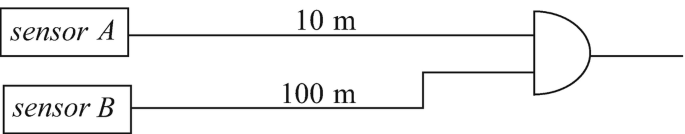
    Figure 16.37

• 16.4 Application: Reflectometry (Narrow Pulses). A lossless cable TV coaxial transmission line is matched to both generator and load. As a routine test, a signal is applied to the input and sent down the line. The distance to the receiver is known to be d = 1 km. The speed of propagation on the line is v_p = c [m/s], and the characteristic impedance on the line is Z₀ = 75 Ω:

  • (a) The signal in Figure 16.38a is obtained on the oscilloscope screen. If Δt = 0.1 μs, what happened to the line and at what location?

  • (b) The signal in Figure 16.38b is obtained on the oscilloscope screen. If Δt = 0.2 μs, what happened on the line and at what location?

    

    Figure 16.38

• 16.5 Application: Reflections on Lossy Line. The cable in Problem 16.4 is given again. However, now the line is considered distortionless, with an attenuation constant of 0.001 Np/m:

  • (a) The signal in Figure 16.38a is obtained on the oscilloscope screen. If Δt = 0.1 μs, what happened to the line and at what location?

  • (b) The signal in Figure 16.38b is obtained on the oscilloscope screen. If Δt = 0.2 μs, what happened on the line and at what location?

  • (c) Compare the location of the fault on the line and magnitude of fault impedance with those for the lossless line in Problem 16.4.

16.1.2 Transients on Transmission Lines: Long Pulses

• 16.6 Transients on an Open Line. A lossless open transmission line is given as shown in Figure 16.39. The line is 10 m long, has capacitance of 200 pF/m and inductance of 0.5 μH/m. Calculate the transient voltage at a distance of 5 m from the DC source:

  • (a) 0.5 μs after closing the switch.

  • (b) 50 μs after closing the switch.

    

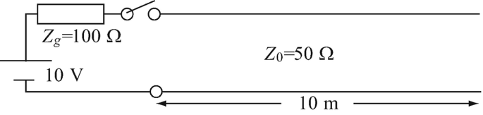
    Figure 16.39

• 16.7 Line Voltage on Long, Loaded Line. A lossless line is very long and the speed of propagation on the line is 10⁸ m/s. Assume the ideal DC source has been switched on. The voltage wave reaches the load at time t₀. Calculate the voltage at point A − A′ (2 m from the load) for t > t₀ and for times t < t₀ (Figure 16.40).

  

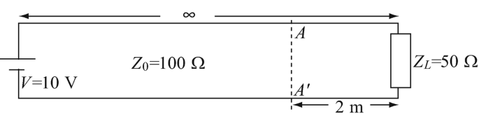
  Figure 16.40

• 16.8 Transient and Steady-State Voltages on Lossless Line. A lossless transmission line of length d [m] is given as in Figure 16.41. The transmission line has capacitance per unit length C₀ [F/m] and inductance per unit length L₀ [H/m]. The switch is closed at time t = 0. Given: L₀ = 10 μH/m, C₀ = 1,000 pF/m, d = 1,000 m, R_g = 100 Ω, R_L = 50 Ω, and V₀ = 100 V:

  • (a) Calculate the steady-state voltage on the line.

  • (b) Calculate the steady-state current in the line.

  • (c) How long does it take the voltage to reach steady state at the load?

  • (d) How long does it take the voltage to reach steady state at the generator?

    

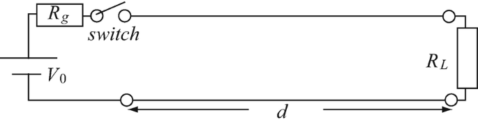
    Figure 16.41

16.1.3 Transients on Transmission Lines: Finite-Length Pulses

• 16.9 Transient Due to a Single Short Pulse. The transmission line in Figure 16.42 is given. The generator supplies a single pulse as shown. Calculate:

  • (a) The voltage and current at the generator 10 μs after the pulse began.

  • (b) The steady-state current and voltage on the line.

    

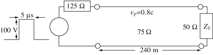
    Figure 16.42

• 16.10 Transient Due to a Single Square Short Pulse on Lossy Line. The circuit in Figure 16.42 is given. In addition to the data in the figure, the line has an attenuation constant α = 0.0001 Np/m. Assume the line is distortionless and calculate the voltage and current at the generator terminals 10.5 μs after the pulse began.

16.1.4 Reflections from Discontinuities

• 16.11 Reflections from Discontinuities. Three sections of lines are connected as shown in Figure 16.43. The propagation time on each section is indicated:

  • (a) If both the load and generator are matched, calculate the line voltage at g, L, and on both sides of the discontinuities a and b, 45 ns after the switch is closed.

  • (b) Same as (a) but the generator impedance is 50 Ω and the load is matched.

    

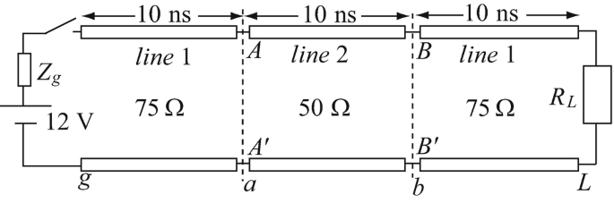
    Figure 16.43

• 16.12 Reflections from Discontinuities. Use the same figure and data as in Problem 16.11. The load now is a short circuit. Given a matched generator, calculate the voltage and current at g, L, and on both sides of the discontinuities a and b, 45 ns after the switch is closed.

16.1.5 Reactive Loading

• 16.13 Application: Capacitively Loaded Transmission Line. A long lossless transmission line with a characteristic impedance of 50 Ω is terminated with a 1 μF capacitor. The length of the line is 100 m and the speed of propagation on the line is c/3 [m/s]. At t = 0, a 100 V matched generator is switched on. Calculate and plot:

  • (a) The load voltage and current for t > 0.

  • (b) The line voltage and current at any point on the line for t > 0.

• 16.14 Application: Inductively Loaded Transmission Line. A long lossless transmission line with characteristic impedance of 50 Ω is terminated with a 1 μH inductor. The line is 10 km long and the speed of propagation on the line is c/3 [m/s]. At t = 0, a 100 V matched generator is switched on:

  • (a) Calculate and plot the load voltage and current for t > 0.

  • (b) Calculate and plot the line voltage and current at any point on the line for t > 0.

16.1.6 Initially Charged Lines

• 16.15 Application: Initially Charged Line. A 300 m long, lossless transmission line has characteristic impedance of 75 Ω and speed of propagation of c/3 [m/s]. The transmission line is matched at the generator and is open ended. The generator’s voltage is 100 V. After the line has reached steady state, the generator is disconnected and a resistor R = 125 Ω is connected across the open end. Calculate and plot the voltage on and the current in R.

• 16.16 Application: Initially Charged Line. A 100 m long lossless transmission line has characteristic impedance of 75 Ω and speed of propagation of 0.2c [m/s]. The transmission line is matched at the generator and is open ended. The generator’s voltage is 100 V. After the line has reached steady state, the generator is disconnected and a resistor R = 125 Ω is connected across the open end:

  • (a) Calculate the voltage on and current in R.

  • (b) How long does it take for the voltage on R to be below 1 V?

16.1.7 Time Domain Reflectometry

• 16.17 Application: Time Domain Reflectometry. An underground cable used for transmission of power has developed a fault. The speed of propagation on the line is known and equal to v_p [m/s]. To locate the fault before starting to dig, time domain reflectometry is performed. A 1 V step pulse is applied to the input with matched impedance and the output in Figure 16.44a is obtained on the oscilloscope. The characteristic impedance of the cable is Z₀ = 50 Ω. Use v_p = 0.2c [m/s] and calculate:

  • (a) The location of the fault.

  • (b) Type of fault: calculate the impedance on the line at the fault.

    

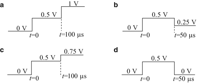
    Figure 16.44

• 16.18 Application: Time Domain Reflectometry. The measurement in Problem 16.17 is performed on a line and the signal in Figure 16.44b is recorded on the time domain reflectometer. Using the data in Problem 16.17, calculate:

  • (a) The location of the fault.

  • (b) Type of fault: calculate the impedance on the line at the fault.

• 16.19 Application: Time Domain Reflectometry. The measurement in Problem 16.17 is performed on a line and the signal in Figure 16.44c is recorded on the time domain reflectometer. Using the data in Problem 16.17, calculate:

  • (a) The location of the fault.

  • (b) Type of fault: find the impedance on the line at the fault.

• 16.20 Application: Time Domain Reflectometry. The measurement in Problem 16.17 is performed on a line and the signal in Figure 16.44d is recorded on the time domain reflectometer. Using the data in Problem 16.17, calculate:

  • (a) The location of the fault.

  • (b) Type of fault: find the impedance on the line at the fault.