The Smith Chart, Impedance Matching, and Transmission Line Circuits

Abstract

A look back at much of what we did with transmission lines reveals that perhaps the dominant feature in all our calculations is the use of the reflection coefficient. The reflection coefficient was used to find the conditions on the line, to calculate the line impedance, and to calculate the standing wave ratio. Voltage, current, and power were all related to the reflection coefficient. The reflection coefficient, in turn, was defined in terms of the load and line impedances (or any equivalent load impedances such as at a discontinuity). You may also recall, perhaps with some fondness, the complicated calculations which required, in addition to the use of complex variables, the use of trigonometric and hyperbolic functions. Thus, the following proposition: Build a graphical chart (or an equivalent computer program) capable of representing the reflection coefficient as well as load impedances in some general fashion and you have a simple method of designing transmission line circuits without the need to perform rather tedious calculations. This has been accomplished in a rather general tool called the Smith chart. The Smith chart is a chart of normalized impedances (or admittances) in the reflection coefficient plane. As such, it allows calculations of all parameters related to transmission lines as well as impedances in open space, circuits, and the like. Although the Smith chart is rather old, it is a common design tool in electromagnetics. Some measuring instruments such as network analyzers actually use a Smith chart to display conditions on lines and networks. Naturally, any chart can also be implemented in a computer program, and the Smith chart has, but we must first understand how it works before we can use it either on paper or on the screen. A computerized Smith chart can then be used to analyze conditions on lines. The examples provided here are solved using graphical tools and a printed Smith chart, rather than the computer program, to emphasize the techniques and approximations involved although some of the numerical results listed were obtained with a computerized Smith chart (smith-chart.m) available with this text (see page xi).

Errors using inadequate data are much less than those using no data at all

—attributed to Charles Babbage (1791–1871)

Designer of the “difference machine” –

the first programmable computing machine and

predecessor to modern computers

Problems

15.1.1 General Design Using the Smith Chart

• 15.1 Application: Line Properties Using the Smith Chart. A long line with characteristic impedance Z₀ = 100 Ω operates at 1 GHz. The speed of propagation on the line is c [m/s] and the load impedance is 260 + j180 Ω. Find:

  • (a) The reflection coefficient at the load.

  • (b) The reflection coefficient at a distance of 20 m from the load toward the generator.

  • (c) Standing wave ratio.

  • (d) Input impedance at 20 m from the load.

  • (e) Location of the first voltage maximum and first voltage minimum from the load.

• 15.2 Application: Calculation of Voltage/Current Along Transmission Lines. A transmission line with a characteristic impedance of 100 Ω and a load of 50 – j50 Ω is connected to a matched generator. The line is very long and the voltage measured at the load is 50 V. Calculate using the Smith chart:

  • (a) Maximum voltage on the line (magnitude only).

  • (b) Minimum voltage on the line (magnitude only).

  • (c) Location of maxima and minima of voltage on the line (starting from the load).

• 15.3 Application: Impedance of Composite Line. A transmission line is made of two segments, each 1 m long (Figure 15.30). Calculate the input impedance of the combined line using a Smith chart if the speed of propagation on line (1) is 3 × 10⁸ m/s and on line (2) 1 × 10⁸ m/s. The lines operate at 300 MHz.

  

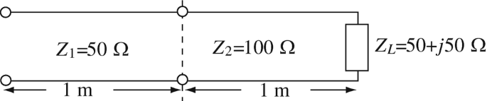
  Figure 15.30

• 15.4 Application: Line Properties. A lossless transmission line has characteristic impedance Z₀ = 300 Ω, is 6.3 wavelengths long, and is terminated in a load impedance Z_L = 35 + j25 Ω. Find:

  • (a) The input impedance on the line.

  • (b) The standing wave ratio on the main line.

  • (c) If the load current is 1 A, calculate the input power to the line.

• 15.5 Application: Line Properties. A lossless transmission line has characteristic impedance Z₀ = 50 Ω and its input impedance is 60 − j70 Ω. The line operates at a wavelength of 0.4 m and is 3.85 m long. Calculate:

  • (a) The load impedance connected to the line.

  • (b) The location of the voltage minima and maxima on the line, starting from the load.

  • (c) The reflection coefficient at the load (magnitude and angle) and the standing wave ratio on the line.

  • (d) The magnitude of the maximum and minimum voltage and current on the line if the load voltage is 22 − j10 V.

• 15.6 Application: Design of Transmission Lines. It is required to design a load of 75 − j50 Ω to simulate a device operating at 100 MHz. It is proposed using a section of a 50 Ω line and connecting to its end a lumped resistance R [Ω]. The line’s phase velocity is c/3 [m/s].

  • (a) Calculate the length of line and the required resistance R that will accomplish this.

  • (b) Is the solution unique? Explain and find all possible solutions if the solution is not unique.

• 15.7 Application: Line Properties Using the Smith Chart. An unknown load is connected to a 75 Ω lossless transmission line. To find the load, two measurements are performed: (1) The location of the first voltage minimum is found at 0.18 λ from the load. (2) The SWR is measured as 2.5. Find using the Smith chart:

  • (a) The load impedance.

  • (b) The load reflection coefficient (magnitude and phase angle).

• 15.8 Application: Evaluation on Line with Unknown Load. A two-wire transmission line with unknown characteristic impedance is 35 m long and connected to an unknown load impedance. Only the input to the line is accessible. To characterize the line and its load, the dimensions of the line are measured as is the input impedance. Each wire is 1.2 mm in diameter and the wires are separated 15 mm apart in air. The input impedance is measured at 915 MHz and found to be Z_in = 350 – j400 Ω and assuming the line is lossless, find:

  • (a) The load impedance.

  • (b) The standing wave ratio on the line.

15.1.2 Stub Matching

• 15.9 SWR on Line. A general load (Z_L = Z₀ + jX_L [Ω]) is connected on a lossless transmission line as shown in Figure 15.31. The shorted section is made of a different line with a different characteristic impedance Z₁ [Ω] and is connected on a lossless transmission line in series with the load.

  • (a) Assuming the generator is matched, calculate the standing wave ratio on the line.

  • (b) What must be the length of the shorted line to ensure matching of the load (no reflection). Are there any other conditions that must be satisfied for this to happen?

    

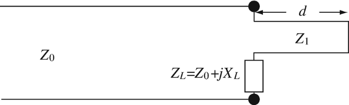
    Figure 15.31

• 15.10 Matching with Shorted/Open Loads. The transmission line network in Figure 15.32 is given. The shorted transmission line and the open transmission line are part of the network. Show that no stub network will match the two line sections to the main line.

  

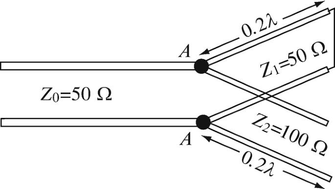
  Figure 15.32

• 15.11 Application: Series Stub Matching. A transmission line of characteristic impedance Z₀ = 50 Ω is loaded with an impedance Z_L = 100 + j80 Ω (Figure 15.33). An open transmission line is connected in series with the line as shown. The open line has the same characteristic impedance as the main line.

  • (a) Find the length of the open series stub and the location (closest to the load) it should be inserted to match the load to the line.

  • (b) Since a stub is a reactive component, find the equivalent lumped component (capacitor or inductor) that can replace the stub found in (a) if the line operates at 500 MHz.

    

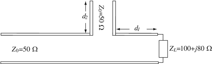
    Figure 15.33

• 15.12 Application: Single Stub Matching. A transmission line is loaded as in Figure 15.34. If the wavelength on the line equals 5 m, find a shorted parallel open and its characteristic impedance is the same as that of the line (location and length of stub) placed to the left of points A–A to match the load to the line.

  

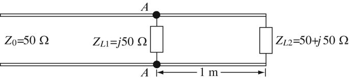
  Figure 15.34

• 15.13 Application: Series Stub Matching. A load is connected to a transmission line as shown in Figure 15.35. It is required to match the load to the line (which has a characteristic impedance of 75 Ω). Find the location and length of a stub to match the line. The stub is open and its characteristic impedance is the same as that of the line as shown in Figure 15.35.

  

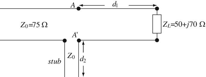
  Figure 15.35

• 15.14 Application: Single Stub Matching. A 75 Ω coaxial cable is used to connect to a TV. The load is matched to the line (Figure 15.36a). A second TV must be connected 10 m from the first TV, again with a 12 m section of the same cable (Figure 15.36b). Assuming the phase velocity on the line is c/2 [m/s], calculate:

  • (a) The reflection coefficient at the location of connection of the two lines.

  • (b) The standing wave ratio on the main line.

  • (c) Design a single stub (its location to the left of the discontinuity and its length) to match the line for TV channel 3 (63 MHz). Use the same line impedance for the stubs.

  • (d) For the design in (c) calculate the reflection coefficient to the left of the stub for channel 2 (57 MHz). What is your conclusion from this calculation as far as stub matching across a range of frequencies?

    

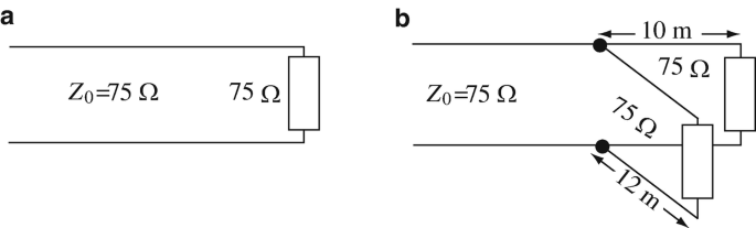
    Figure 15.36

• 15.15 Application: Single Stub Matching of a Generator. Consider the problem of matching a generator with internal impedance of 50 Ω to a line with characteristic impedance of 75 Ω. Find the length (l) of a parallel stub and the distance of the stub (d) from the generator terminals that will achieve the required match (see Figure 15.37). Comment on the behavior of the forward and backward waves on the line to the right and to the left of the stub.

  

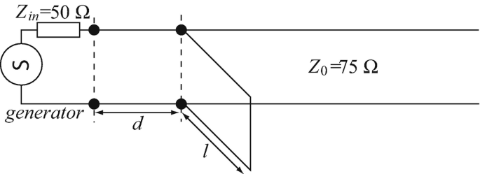
  Figure 15.37

• 15.16 Application: Double Stub Matching. Two stubs are used on a transmission line as shown in Figure 15.38. Calculate stub lengths d₁ and d₂ (in wavelengths) to match the load to the line. Is this arrangement of stubs a good arrangement? Why?

  

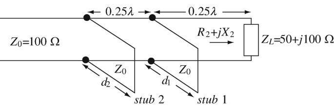
  Figure 15.38

• 15.17 Application: Double Stub Matching. An antenna has an impedance of 68 + j100 Ω. The antenna needs to be connected to a 75 Ω line. Because the antenna goes on a mast, the design engineer decided to fabricate a matching section as shown in Figure 15.39. The matching section is then connected to the antenna during installation. At the required frequency, the section is 0.3 λ long and the two stubs are made of 75 Ω line sections. Calculate the lengths of the stubs, if the antenna is connected at A − A.

  

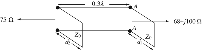
  Figure 15.39

15.1.3 Transformer Matching

• 15.18 Application: λ/4 Transformer. Show that two lines with any characteristic (real) impedances Z₁ [Ω] and Z₂ [Ω] may be matched with a quarter-wavelength line. What is the characteristic impedance of the matching section?

• 15.19 Application: 3λ/4 Transformer. A lossless transmission line with characteristic impedance Z₀ [Ω] transfers power to a load Z_L [Ω] (real). To match the line, a matching section is connected as shown in Figure 15.40. At what distance d (in wavelengths) from the load must the line be connected (minimum distance) and what must the characteristic impedance of the matching section be?

  

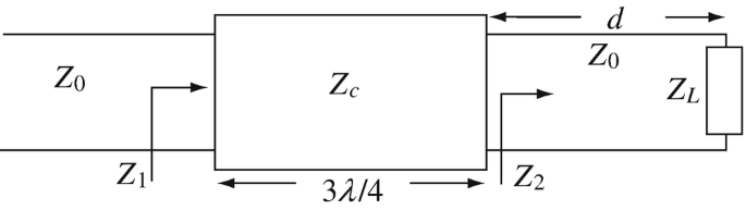
  Figure 15.40

• 15.20 Application: λ/4 Transformer. A transmission line is given as shown in Figure 15.41. If the characteristic impedance of the quarter-wavelength transformer must be real, find the location of the transformer (distance d in the figure, in wavelengths) and the intrinsic impedance of the transformer Z_t [Ω].

  

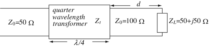
  Figure 15.41

• 15.21 Application: λ/4 Transformer. A two-wire transmission line has characteristic impedance of 300 Ω and connects to an antenna. The line is long and the antenna has an impedance of 200 Ω and operates at a wavelength of 3.8 m. To match the line and load, a quarter-wavelength transformer is connected on the line, but the location at which the transformer may be connected is 10 m from the antenna or larger. Calculate:

  • (a) The closest location at which the transformer may be connected.

  • (b) For the result in (a), the characteristic impedance of the transformer section.

  • (c) The standing wave ratios on the sections of line between the transformer and antenna and between transformer and generator.

• 15.22 Application: λ/4 Transformer Matching at Load and Generator. A 75 Ω transmission line is connected at one end to a generator with internal impedance Z_in = 50 − j75 Ω and on the other end to a load of impedance Z_L = 100 + j75 Ω.

  • (a) Design a λ/4 transformer to match the generator to the line; specify the minimum distance from the generator and its characteristic impedance.

  • (b) Design a λ/4 transformer to match the load to the line; specify the minimum distance from the load and its characteristic impedance.

• 15.23 Application: Imperfect Transformer Matching. A λ/4 transformer can only match exactly at the frequency at which it is exactly λ/4.

  A λ/4 transformer is designed to operate at 2.4 GHz to match a 24 + j40 Ω load to a 50 Ω lossless transmission line.

  • (a) Find the lowest possible characteristic impedance of the transformer and the distance from the load at which it must be located to match the load to the line at 2.4 GHz.

  • (b) If the frequency changes to 1.9 GHz, calculate the standing wave ratio to the left of the transformer designed in (a).