Theory of Transmission Lines

Abstract

Hopefully, by now you have a good understanding of waves propagating in space and in materials, including reflection and transmission at interfaces. Although not mentioned often enough, there were a number of assumptions implicit in this type of propagation. The most important was the fact that only plane waves were treated. In most cases, we also assumed the waves only propagate forward from the source, although reflections from interfaces cause waves to also propagate backward toward the source and these were treated in Chapter 13. While the existence of interfaces complicates treatment, it also allows for applications such as radar to be feasible. If we were to summarize the previous two chapters in a few words, we would say that all wave phenomena were treated in essentially infinite space; that is, plane waves were not restricted in space except for the occasional interface.

O tell me, when along the line

From my full heart the message flows,

What currents are induced in thine?

One click from thee will end my woes.

—James C. Maxwell (1831–1879),

mathematician, physicist

Valentine from a telegraph clerk to a telegraph clerk,

Problems

14.1.1 Transmission Line Parameters

• 14.1 Application: Coaxial Transmission Line. Two coaxial transmission lines, each made of an inner and an outer conducting shell, are given. The radius of the inner shell is a = 10 mm and the radius of the outer shell is b = 20 mm. The lines are shown in cross section in Figure 14.31. Permittivity and permeabilities are given. Calculate the line parameters for each line assuming perfect conductors.

  

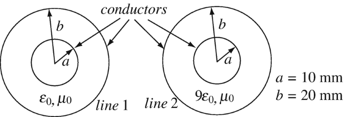
  Figure 14.31

• 14.2 Application: Overhead Transmission Line with Ground Return. Two students live 1 km apart. They decide to connect between them a line so that they may use a private telephone without having to pay for the service. To do so, they need a transmission line and this requires two conductors. Since they do not have enough money, they decide to use a single wire and use the ground as the return conductor, assuming the ground is a good conductor. The wire is 1 mm thick and is strung at a height of 5 m above ground.

  • (a) Is this a sound approach?

  • (b) If so, calculate the line parameters for the transmission line made of the single conductor and ground, assuming a perfectly conducting ground.

  • (c) Suppose the installation was a bit flimsy and during a storm, their wire fell to the ground. The wire is insulated and the insulation is 0.5 mm thick. What are the line parameters now? Use permittivity and permeability of free space for the insulating material.

14.1.2 Long, Lossless Lines

• 14.3 Application: Parameters of Coaxial Line. The RG-11/U coaxial line has the following properties: Z₀ = 75 Ω, v_p = 2c/3 m/s. Assuming the line to be lossless, calculate its inductance and capacitance per unit length.

• 14.4 Application: Coaxial Line and Delay on the Line. A coaxial transmission line is made of two circular conductors as shown in Figure 14.32. The inner conductor has diameter b and the outer conductor diameter a. The conductors are perfect conductors and are separated by a lossless ferrite (a material with finite permeability, finite permittivity, and zero conductivity). Given: ε₀ = 8.854 × 10⁻¹² F/m, μ₀ = 4π × 10⁻⁷ H/m, ε₁ = 9ε₀ [F/m], μ₁ = 100μ₀ [H/m], a = 8 mm, b = 1 mm.

  • (a) Calculate the characteristic impedance and the phase velocity on the line.

  • (b) Two coaxial transmission lines connect two memory banks to a processor. Line A is the same as calculated in part (a). Line B has the same dimensions, but the ferrite is replaced with free space. What must be the minimum execution cycle (maximum frequency) of the processor if the two memory signals must reach the processor within one execution cycle. Assume the length of each line is d = 100 mm. The execution cycle is defined by the slower of the signals.

    

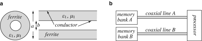
    Figure 14.32

• 14.5 Application: Microstrip Line. A conducting strip with dimensions as shown in Figure 14.33 is located above a conducting surface. The strip is very long and the conducting surface is infinite. Also, w ≫ d. The strip and surface serve as a transmission line. Calculate assuming perfect conductors:

  • (a) Speed of propagation of waves on this line.

  • (b) Characteristic impedance of the transmission line for w = 10 mm, and d = 0.1 mm.

    

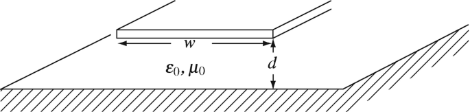
    Figure 14.33

14.1.3 The Distortionless Transmission Line

• 14.6 Application: The Distortionless Line. A coaxial line is made as shown in Figure 14.34. Material properties and dimensions are given in the figure. The design calls for a distortionless transmission line at 250 MHz.

  • (a) Assuming the outer radius must remain constant (b = 20 mm), what must be the radius a of the inner conductor for the line to be distortionless? Assume material properties μ₀ [H/m], ε₀ [F/m], σ_c = 5.7 × 10⁷ [S/m] for copper.

  • (b) What is the characteristic impedance of the line and what is its attenuation constant for the design in (a)?

  • (c) If reduction of at most 10 dB in amplitude is allowed before an amplifier is required, calculate the distance between each two amplifiers on the line.

    

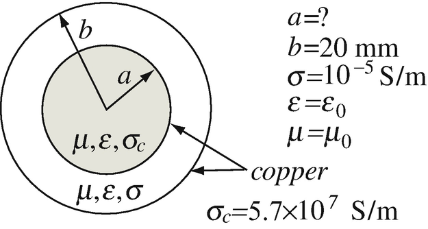
    Figure 14.34

• 14.7 Application: Distortionless Parallel Plate Line. A parallel plate line is made as shown in Figure 14.35. Material properties and dimensions are given in the figure. The design calls for a distortionless transmission line operating at 1,000 MHz.

  • (a) Calculate the required distance d between the two conductors to produce a distortionless line at the given frequency.

  • (b) What are the characteristic impedance and attenuation constant of the line?

  • (c) If a reduction of at most 75 dB in amplitude is allowed before an amplifier is required, calculate the distance between each two amplifiers on the line.

    

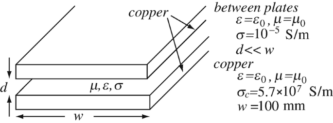
    Figure 14.35

14.1.4 The Low-Resistance Transmission Line

• 14.8 Application: Low-Resistance Power Line. A power line is made of two round, parallel conductors, 20 mm in diameter, separated by 0.8 m, and suspended above ground, in air. Neglect any ground effects. Properties of air are: ε₀ [F/m], μ₀ [H/m], σ = 10⁻⁵ S/m. The line is made of aluminum (μ = μ₀ [H/m], ε = ε₀ [F/m], σ_c = 3.5 × 10⁷ S/m) and operates at 60 Hz. Calculate:

  • (a) The propagation constant on the line. Show that this may be assumed to be a low-resistance line.

  • (b) Under the assumption of a low-resistance line, calculate the characteristic impedance of the line and its attenuation and phase constants.

• 14.9 Application: Properties of Telephone Lines. A two-wire, open-air telephone line is made of round wires, 1 mm in radius, and are supported 200 mm apart on insulating cups.

  The line is made of copper, with conductivity of 5.7 × 10⁷ S/m, and the surrounding space is air (with properties of free space). The line is 3 km long, may be assumed to be low loss, and is used to transmit data at 10 kHz.

  • (a) What is the load impedance if it must equal the characteristic impedance of the line?

  • (b) If the load requires 0.01 W to operate, how much power must be supplied to the line input?

  • (c) Suppose you are free to adjust the distance between the lines. Can the line be redesigned to be distortionless? If so, how?

  • (d) Is the assumption that the line is a low-loss line justified? Explain.

• 14.10 Properties of Long Lines. A long line has parameters R, L, C, G = 0, and operates at 100 kHz. The characteristic impedance is Z₀ = 300 − j10 Ω and the phase velocity on the line is v_p = 2c/3 m/s. Find:

  • (a) The values of R, L, and C assuming the line is a low-loss line.

  • (b) Calculate the propagation constant on the line.

  • (c) Is the assumption in (a) that the line is low loss justified?

14.1.5 The Field Approach to Transmission Lines

• 14.11 Application: Power Relations on Coaxial Lines. Coaxial lines are usually used for transmission of signals at high frequencies. In some cases however, the lines are also required to carry considerable power at lower frequencies. One example is the cable TV coaxial line. These carry both the high-frequency video signals and 60 Hz power to operate devices on the line (such as amplifiers). Typical requirements are for the lines to carry up to 10 A at about 60 V. Consider the following example:

  A coaxial cable with the dimensions shown in Figure 14.36 has a characteristic impedance of 75 Ω. The line is connected to an AC source at 60 V (peak), 60 Hz. Neglect internal impedance in the source. The line may be considered long and the load is matched to the line. Calculate:

  • (a) The electric and magnetic field intensities in the dielectric of the line.

  • (b) Show that application of the Poynting theorem anywhere on the line gives the same time-averaged power as that obtained from the current voltage relations.

    

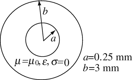
    Figure 14.36

• 14.12 Application: Exposure to Electromagnetic Fields. One recent health concern is with exposure to both low- and high-frequency electromagnetic fields. These are believed by some to cause cancer. An AM station transmitting at 1 MHz decided to minimize exposure of personnel due to power on the transmission line leading from the generator to the antenna. The transmission line is a two-wire exposed (no insulation) line, 10 mm in diameter and separated by 0.2 m. The transmission line is parallel to the ground and leads to an antenna located at some distance from the transmitter, on top of a hill. The station decided that to minimize the risk due to the fields generated by the line, it will not allow the peak magnetic flux density at a distance 1 m from the center of the transmission line to exceed 10⁻⁶ T.

  • (a) What is the peak power the station can transmit without violating the maximum magnetic flux density requirement? Assume a lossless line and matched conditions at load and generator. Neglect effects due to the ground.

  • (b) Suppose the station needs to transmit more power than allowed in (a). To do so, the engineers decide to move the two wires closer together so that now they are 0.1 m apart. How much power can the station transmit now without violating the maximum field requirement?

  • (c) What are the peak electric field intensities in (a) and (b) at the location of the peak magnetic flux density?

14.1.6 Finite Transmission Lines

• 14.13 Application: Voltage and Current on Transmission Lines. The voltage and current at the center of the lossless line in Figure 14.37 are given as V_c=18 V, I_c=0.2 A. If the wavelength is 1 m, calculate:

  • (a) The forward- and backward-propagating voltages.

  • (b) The forward- and backward-propagating currents.

  • (c) The load impedance.

    

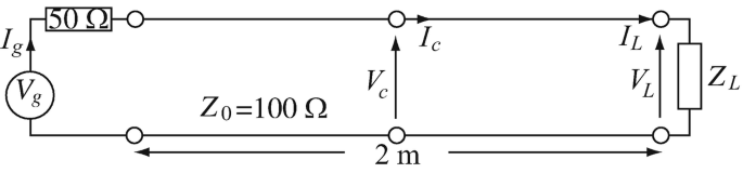
    Figure 14.37

• 14.14 Application: Voltage and Current on Transmission Lines. The voltage and current at the load of the lossless line in Figure 14.37 are given as V_L = 50 V, I_L = 0.2 A. If the wavelength is 1 m, calculate:

  • (a) The voltage and current of the generator.

  • (b) The power supplied by the generator.

• 14.15 Multiple Loads on a Line. A lossless transmission line with characteristic impedance of 100 Ω is connected to a generator and three loads as shown in Figure 14.38 are connected to the line. Calculate:

  • (a) The power dissipated in each of the loads if the amplitude of the voltage across load (2) is given as 12 V.

  • (b) The power supplied by the generator to the line.

  • (c) The power dissipated in the generator itself.

    

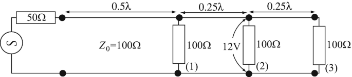
    Figure 14.38

• 14.16 Application: Terminated Line, Matched Power Transfer. A load impedance Z_L = 50 Ω is connected to a generator of impedance Z_G = 50 Ω through a lossless transmission line with characteristic impedance Z₀ = 200 Ω.

  • (a) What must be the length d of the line (in wavelengths) for matched power transfer from generator to load?

  • (b) If the characteristic impedance of the line is changed to Z₀ = (200 + j91) Ω, what is the length of the line (in wavelengths) for matched power transfer between generator and load?

  • (c) Show that at any value of d other than those found in (a) or (b), the load is not matched to the generator.

• 14.17 Terminated, Mismatched Line. The line in Figure 14.39 is given. The generator can be connected anywhere on the line. It is required that the generator be matched to the line so that there are no reflections into the generator. Find the closest location d (in wavelengths) to the load at which you can move the generator so that the generator is best matched to the line (i.e., the reflection coefficient at the generator is minimum). Assume the phase constant on the line is known as β₀ [rad/m].

  

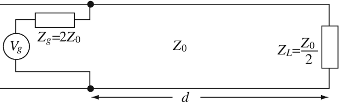
  Figure 14.39

14.1.7 Line Impedance, Reflection Coefficient, Etc

• 14.18 Generalized Reflection Coefficient on a Line. Calculate the generalized reflection coefficient and the line impedance at a distance a wavelengths from the discontinuity shown in Figure 14.40. Assume the generator is matched to the line but the load is not. Dimensions are in wavelengths.

  

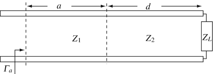
  Figure 14.40

• 14.19 Application: Input Impedance of Striplines. A transmission line is made of two strips separated a distance d [m]. The width of the strips is w [m] and their thickness is b [m]. The strips are made of a conductor with conductivity σ [S/m]. The material between the strips is air (free space). A load Z_L [Ω] is connected at one end of the line (see Figure 14.41). Calculate the input impedance of the line at a distance r = 1.8 wavelengths from the load. Given: w ≫ d, σ_c = 1.0 × 10⁷ S/m, w = 20 mm, d = 0.5 mm, b ≫ δ, μ = μ₀ [H/m], ε = ε₀ [F/m], Z_L = 75 Ω, f = 1 GHz.

  

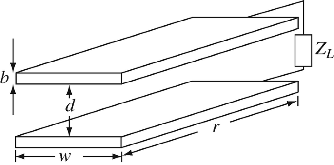
  Figure 14.41

• 14.20 Line Impedance on Line with Multiple Loads. The lossless transmission line in Figure 14.42 represents a distribution line and a load that has been shorted at its end as shown. Calculate the line impedance at a distance of 0.5λ to the left of the load.

  

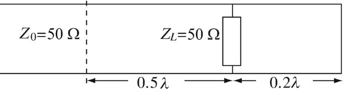
  Figure 14.42

• 14.21 Line Impedance on Line with Multiple Loads. The transmission line in Figure 14.43 is a distribution line normally operating at matched conditions. A second load at the end of the line has opened inadvertently. Calculate the line impedance at a distance 0.25λ from the load as shown.

  

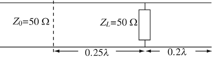
  Figure 14.43

• 14.22 Voltage and Power on Lossless Line. A 75 Ω, lossless transmission line is connected on one side to a generator and the other to a load. The generator has internal impedance of 150 Ω and open circuit voltage amplitude of 24 V. Wavelength is 0.32 m and the line is 125 m long. The load is an antenna with impedance 75 + j42 Ω. Calculate:

  • (a) The voltage at the load.

  • (b) The power supplied to the line by the generator.

• 14.23 Connection of Transmission Lines in Parallel. A lossless transmission line with characteristic impedance of 50 Ω is connected as shown in Figure 14.44. The measured impedance between points A–A′ is 100 Ω. Calculate the two impedances Z_L1 and Z_L2 if the input impedance of the two lines when disconnected is equal.

  

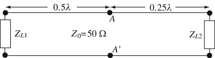
  Figure 14.44

14.1.8 Shorted and Open Transmission Lines

• 14.24 Open and Shorted Transmission Lines. The two configurations in Figure 14.45 are given. The lines are lossless with air as insulator between the lines and operate at 300 MHz. The voltage of the generator is 12 V rms.

  • (a) Calculate the current supplied by the generator in Figure 14.45a.

  • (b) Calculate the current supplied by the generator in Figure 14.45b.

  • (c) How much power does the generator supply in (a) and in (b)? Explain.

  • (d) What are the answers to (a) and (b) if the frequency is doubled to 600 MHz?

  • (e) What are the answers to (a) and (b) if the frequency is halved to 150 MHz?

    

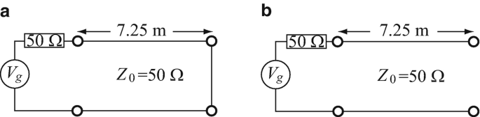
    Figure 14.45

• 14.25 Application: Design of Network Elements. In the design of a transmission line network, it is required to design a reactance of j100 Ω as an element in the network. Show how this can be accomplished with:

  • (a) A lossless, shorted transmission line with characteristic impedance of 50 Ω at a wavelength of 1 m.

  • (b) A lossless open transmission line with characteristic impedance of 75 Ω at a wavelength of 1 m.

  • (c) If a capacitive reactance of − j100 Ω is needed instead, what are the answers to (a) and (b)?

• 14.26 Application: Experimental Evaluation of Line Parameters. A transmission line is 10 km long and operates under matched conditions. An engineer requires the properties of the line; that is, its characteristic impedance, its attenuation constant, and its phase constant. It is not possible to subject the line to testing equipment, but the voltage and currents can be measured at the load and at the generator. These are given as V = 10 V, I = 0.1 A at the generator and V = 3 − j2 V at the load. Find:

  • (a) The characteristic impedance, attenuation, and phase constants on the line.

  • (b) The time-averaged power loss on the line.

• 14.27 Application: Measurements of Line Conditions. A lossless transmission line is connected to a matched load. The characteristic impedance of the line is 50 Ω. An additional load is connected to the line. To determine the additional load, the maximum voltage on the line is measured as 48 V and the minimum voltage on the line is measured as 30 V. From these measurements, calculate:

  • (a) The additional load connected across the matched load.

  • (b) What are the maximum and minimum line impedances and where do these occur?

• 14.28 Line Conditions on Shorted and Open Lines. The standing wave ratio on a lossless transmission line is measured and found to be infinite.

  • (a) Can you tell from this measurement if the load is a short or an open circuit? Explain.

  • (b) Suppose you can measure the line impedance directly and you find that at one point, the line impedance is zero. Moving toward the load a very short distance, you find that the line impedance is purely reactive and increases. Can you now tell if the line is shorted or open? If so, how?

• 14.29 Design with Open and Shorted Transmission Lines. The filter shown in Figure 14.46 needs to be implemented with transmission line segments so that it may be inserted in a line circuit. Show how this may be done and calculate the line segment lengths in your implementation. The lines are lossless two-wire lines with air as insulator and a characteristic impedance of 75 Ω. Assume that the distance between the two wires in the line segments is very small compared to the wavelength. The frequency of operation is 450 MHz. Note that there is more than one solution possible.

  

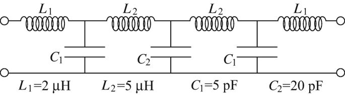
  Figure 14.46

14.1.9 Resistive Loads on Transmission Lines

• 14.30 Application: Standing Wave Ratio Measurements. On a lossless transmission line, SWR = 5 and Z₀ = 50 Ω. To identify the conditions on the line, three measurements are made by sliding a voltmeter along the line. (1) The first maximum is found at a distance 0.25 m from the load. (2) The next maximum is found at 0.75 m from the load. (3) V_L = 100 V. Calculate:

  • (a) The load impedance.

  • (b) The amplitudes of the forward- and backward-propagating voltage waves.

  • (c) The amplitudes of the forward- and backward-propagating current waves.

• 14.31 Application: Standing Wave Ratio and Minima and Maxima on the Line. For a line with characteristic impedance Z₀ = 50 Ω and a load R = 220 Ω, calculate:

  • (a) The standing wave ratio on the line.

  • (b) If the voltage at the load is 100 V, find the maximum and minimum voltage on the line.

  • (c) Where do the voltage maxima and minima occur?

• 14.32 Application: Power Supplied to Resistively Loaded Line. Two lossless transmission line segments are connected as shown in Figure 14.47. Calculate the power supplied by the generator to the line.

  

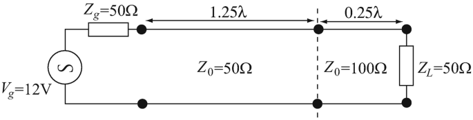
  Figure 14.47

• 14.33 Application: Measurement of Characteristic Impedance. To measure the characteristic impedance of a lossless transmission line it is proposed to measure the voltage at the load and at a distance d [m] from the load. The line is made of two wires in free space (air) and is connected to a 100 Ω load. The voltage at the load is measured as 50 V and at a distance d it is 120 V.

  • (a) Calculate the characteristic impedance of the line.

  • (b) If the line operates at a wavelength of 1.8 m, what is the distance d?

• 14.34 Application: Standing Wave Ratio and Minima and Maxima on the Line. A lossless line has a characteristic impedance Z₀ = 50 Ω and a load R = 25 Ω. Calculate:

  • (a) The standing wave ratio on the line.

  • (b) If the voltage at the load is 100 V, find the maximum and minimum voltage on the line.

  • (c) Where do the voltage maxima and minima occur?

14.1.10 Capacitive and Inductive Loads on Transmission Lines

• 14.35 Application: Line Impedance on a Capacitively Loaded Line. A long lossless transmission line with characteristic impedance 50 Ω is terminated with a capacitance. At the frequency at which the line operates, the impedance of the load is − j50 Ω and the phase constant on the line is 20π [rad/m]. Calculate and plot the line impedance as a function of distance from load.

• 14.36 Application: Line Impedance on an Inductively Loaded Line. A long lossless transmission line with characteristic impedance 50 Ω is terminated with an inductance. At the frequency at which the line operates, the reactance of the load is 50 Ω and the phase constant is 20π [rad/m]. Calculate and plot the line impedance as a function of distance from load.

• 14.37 Line Impedance on Line with General Load. A long lossless transmission line with characteristic impedance 50 Ω is terminated with a load as in Figure 14.48. The line operates in free space (material between the two lines is air) at 1 MHz. Calculate:

  • (a) The generalized reflection coefficient on the line.

  • (b) The standing wave ratio on the line.

  • (c) The location of the first minimum voltage on the line.

  • (d) The standing wave ratio as a function of frequency. Plot for frequencies between 0.5 and 1 MHz.

    

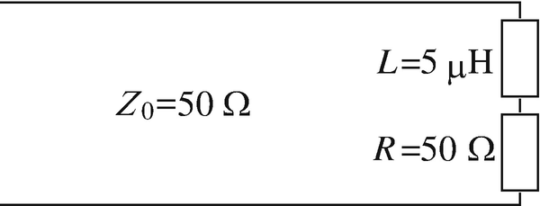
    Figure 14.48

• 14.38 Line Impedance on Line with General Load. A long lossless transmission line with characteristic impedance 50 Ω is terminated with a load as in Figure 14.49. The line operates in free space (material between the two lines is air) at 1 MHz. Calculate:

  • (a) The generalized reflection coefficient on the line.

  • (b) The standing wave ratio on the line.

  • (c) The location of the first minimum voltage on the line.

  • (d) The standing wave ratio as a function of frequency. Plot for frequencies between 0.5 and 1 MHz.

  

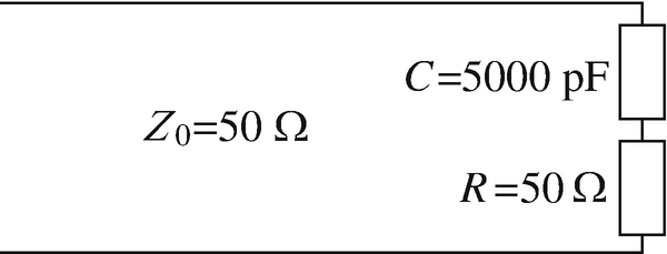
  Figure 14.49

14.1.11 Power Relations on Transmission Lines

• 14.39 Power on Lossless Line. A lossless transmission line is given as shown in Figure 14.50. Calculate the power dissipated in the load. The generator is matched to the line and has a voltage of 100 V rms.

  

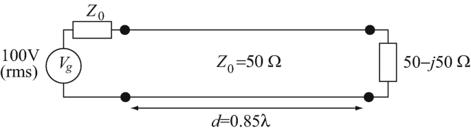
  Figure 14.50

• 14.40 Voltage and Power on a Coaxial Line. A coaxial line is made as follows (Figure 14.51): The inner wire diameter is 0.5 mm and the outer one is 6 mm. The material between the conductors is a polymer with relative permittivity 4 and conductivity 10⁻⁷ S/m. The line is matched at generator and load and is used as a cable TV line at 100 MHz. The peak input voltage to the line is 10 V and the line is 200 m long. Assuming ideal conductors, calculate:

  • (a) The voltage at the load.

  • (b) The time averaged power loss on the line.

    

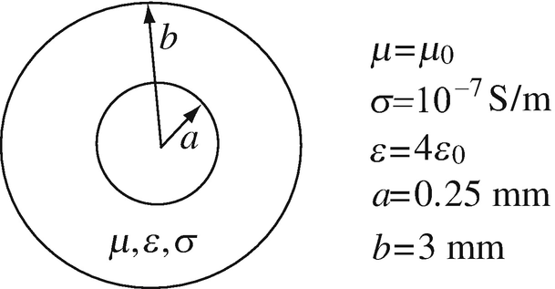
    Figure 14.51

• 14.41 Application: Power Loss on Lossy Transmission Line. A distortionless transmission line has the following parameters:

  $$ R=0.2\kern0.5em \left[\Omega /\mathrm{m}\right],L=1\kern0.5em \left[\upmu \mathrm{H}/\mathrm{m}\right],G={10}^{-5}\kern0.5em \left[\mathrm{S}/\mathrm{m}\right],C=50\kern0.5em \left[\mathrm{pF}/\mathrm{m}\right] $$

  The line is matched at the load and is 12.2 wavelengths long at a frequency of 120 MHz. If a power P₀ [W] is supplied at its input terminals, what is the percentage of power lost on the line?

• 14.42 Power on Lossy Line. In the line shown in Figure 14.52 it is required that the load dissipates 10 W. Calculate the net power entering the line at location A to produce the required power in the load. Note: net power means the power that propagates towards the load and is the difference between the forward propagating power and the backward propagating power.

  

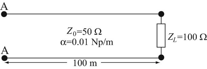
  Figure 14.52

• 14.43 Power Transfer on Lossy Line. A lossy 2-wire transmission line with an attenuation constant α = 0.1 Np/m is matched at the generator. That is, Z_g = Z₀ = 50 Ω. The load is Z_L = 100 Ω. The medium between the wires is air. The line operates at a wavelength of 0.5 m. The voltage at a distance d = 3.2 wavelengths from the load is measured as V = 100 V. Calculate the power delivered to the load.

14.1.12 Resonant Transmission Lines

• 14.44 Application: Transmission Line Resonator. A transmission line resonator is made by connecting a 10 pF capacitor across the input of a 75 Ω lossless line and shorting the other end (Figure 14.53). What must be the length of the line in wavelengths so that the lowest resonant frequency is 100 MHz?

  

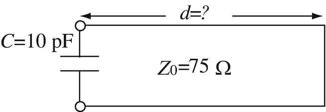
  Figure 14.53

• 14.45 Application: Transmission Line Resonator. A lossless transmission line is cut into a length b = 0.5 m and shorted at both ends (Figure 14.54). Properties of the line are Z₀ = 75 Ω and v_p = c/3 [m/s].

  • (a) If a connection is made at a point x = b/2, what is the impedance of the line at this point?

  • (b) A connection is now made on the line such that x = 0.1 m. Find the first four resonant frequencies for this line.

    

    Figure 14.54

• 14.46 Application: Transmission Line Sensors. A transmission line resonator is made as shown in Figure 14.55. The device is used to sense moisture content of dough on a production line as the dough passes through the device, given as a percentage. Dough has a permittivity given by ε = ε₀(1 + 14k) [F/m], where k is the percentage of water in the dough. Calculate:

  • (a) The resonant frequency of the device when empty.

  • (b) The resonant frequency for 15%, 10%, and 5% moisture in the dough.

  • (c) Comment on the applicability of this design for moisture measurements.

    

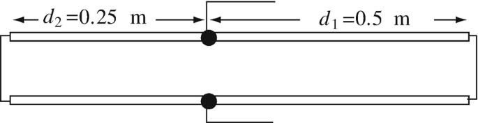
    Figure 14.55

• 14.47 Application: Detection of Faults in Buried Lines. A buried cable has been cut at an unknown point. A signal generator is connected to the cable input and the frequency is swept. The first maximum at the generator occurs at a frequency f₁ [Hz] and the first minimum at a frequency f₂ > f₁. What is the distance from the generator to the short if the phase velocity is known and equals v_p0 [m/s] at both frequencies. The generator is matched to the line.

• 14.48 Application: Detection of Faults in Buried Lines. A buried cable has water leaking into it, at a location along its length. The water leak manifests itself as an unknown impedance on the cable at the location of the leak. If the same results as in Problem 14.47 are obtained at the generator:

  • (a) Is it possible with the data given in Problem 14.47 to find the exact location of the leak?

  • (b) If yes, what is that location? If not, what is the minimum section that must be dug to ensure that the leak is found?