Electromagnetic Waves and Propagation

Abstract

After summarizing Maxwell’s equations in Chapter 11, we are now ready to discuss their implications. In particular, we will deal directly or indirectly with the displacement current term in Maxwell’s equations.

As to the properties of electromagnetic radiation, I need first of all to come up with a little more than just words to the idea that a changing magnetic field makes an electric field, a changing electric field makes a magnetic field and that this pumping cycle produces an electromagnetic wave…

J. Robert Oppenheimer (1904–1967), physicist

from The Flying Trapeze, Oxford University Press, 1964

Problems

12.1.1 The Time-Dependent Wave Equation

• 12.1 The Wave Equation. Starting with the general time-dependent Maxwell’s equations in a linear, isotropic, homogeneous medium, write a wave equation in terms of the electric field intensity.

  • (a) Show that if you neglect displacement currents, the equation is not a wave equation.

  • (b) Write the source-free wave equation from the general equation you obtained.

• 12.2 Source-Free Wave Equation. Obtain the source-free time-dependent wave equation for the magnetic flux density in a linear, isotropic, homogeneous medium.

12.1.2 The Time-Harmonic Wave Equation

• 12.3 Time-Harmonic Wave Equation. Using the source-free Maxwell’s equations, show that a Helmholtz equation can be obtained in terms of the magnetic vector potential. Use the definition B = ∇ × A and a simple medium (linear, isotropic, homogeneous material). Justify the choice of the divergence of A.

• 12.4 The Helmholtz Equation for D. Using Maxwell’s equations, find the Helmholtz equation for the electric flux density D in a linear, isotropic, homogeneous material.

• 12.5 The Electric Hertz Potential. In a linear, isotropic, homogeneous medium, in the absence of sources, the Hertz vector potential Π_e may be defined such that H = jωε∇ × Π_e:

  • (a) Express the electric field intensity in terms of Π_e.

  • (b) Show that the Hertz potential satisfies a homogeneous Helmholtz equation provided a correct gauge is chosen. What is this appropriate gauge?

12.1.3 Solution for Uniform Plane Waves

• 12.6 Plane Wave. The electric field intensity of a plane wave has an amplitude of 120 V/m, is directed in the negative z direction, has a frequency of 76 MHz and propagates in the positive y direction in free space (properties of free space are ε = ε₀ [F/m], μ = μ₀ [H/m].)

  • (a) Write the expression of the electric field intensity in phasor and time-dependent forms.

  • (b) Write the expression for the magnetic field intensity in phasor and time-dependent forms.

• 12.7 Plane Wave. A wave propagates in free space and its electric field intensity is $\mathbf{E}=\hat{\mathbf{x}}100{e}^{-j220z}+\hat{\mathbf{x}}100{e}^{j220z}\;\left[\mathrm{V}/\mathrm{m}\right]$:

  • (a) Show that E satisfies the source-free wave equation.

  • (b) What are the wave’s phase velocity and frequency?

12.1.4 The Poynting Vector

• 12.8 Use of the Poynting Vector. A simple and common use of the Poynting vector is identification of direction of propagation of a wave or the direction of fields in space. Consider the magnetic field intensity of a plane electromagnetic wave propagating in free space:

  $$ \mathbf{H}=\hat{\mathbf{x}}{H}_0{e}^{j\beta y}+\hat{\mathbf{z}}{H}_1{e}^{j\beta y}\kern1em \left[\mathrm{A}/\mathrm{m}\right] $$

  • (a) Calculate the electric field intensity using the properties of the Poynting vector.

  • (b) Show that the result in (a) is correct by substituting the magnetic field intensity into Maxwell’s equations and evaluating the electric field intensity through Maxwell’s equations.

• 12.9 Application: Power Relations in a Microwave Oven. The peak electric field intensity at the bottom of a microwave oven is equal to 2,500 V/m. Assuming that this is uniform over the area of the oven which is equal to 400 cm², calculate the peak power the oven can deliver. Permeability and permittivity are those of free space.

• 12.10 Application: Heating Food in a Microwave Oven. A frozen pizza is marketed to be heated in a microwave oven. As an engineer you are asked to write heating instructions, specifically how long should it be heated to reach a proper temperature. The average residential microwave oven is 50 cm wide, 40 cm deep, and 30 cm high. The oven has a low and a high heating level. At low, it produces a time averaged power of 500 W, whereas at high, the power is 1000 W. We will assume the pizza is placed flat on the bottom of the oven and any power coupled into the pizza enters from above. The pizza is 25 cm in diameter, 1.5 cm thick, and is 75% water by volume. The microwave oven heats the water in the pizza. The frozen pizza is at –20 °C and must be heated to 75 °C. Heat capacity of water is 4.1885 J/(g⋅K) and the latent heat (of melting ice) is 334 J/g (heat capacity is the energy needed to raise the temperature of one gram of substance (water in this case) by 1 degree Kelvin, and latent heat is the energy required to melt a gram of ice at 0 °C to water at 0 °C). Assume that the heat transfer from the electromagnetic waves to the pizza is 80% efficient and calculate:

  • (a) The time it takes to heat the pizza on the low setting of the oven.

  • (b) The time it takes to heat the pizza on the high setting of the oven.

  • (c) The cost in electricity to heat the pizza if a kW⋅h costs $0.16.

• 12.11 Application: Power Dissipation in Cylindrical Conductor. A cylindrical conductor of radius R and infinite length carries a current of amplitude I [A] and frequency f [Hz]. The conductivity of the conductor is σ [S/m] (Figure 12.23). Calculate the time-averaged dissipated power per unit length in the conductor, neglecting displacement currents in the conductor. Assume the current is uniformly distributed throughout the cross section.

  

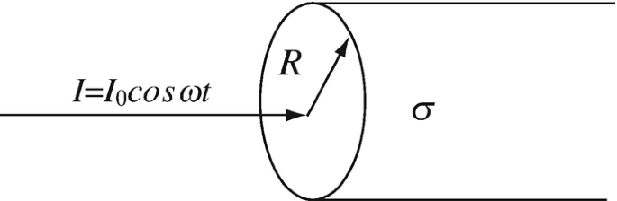
  Figure 12.23

• 12.12 Application: Power Radiated by an Antenna. An antenna produces an electric field intensity in free space as follows:

  $$ \mathbf{E}=\hat{\boldsymbol{\uptheta}}\frac{12\pi }{R}{e}^{-j2\pi R}\sin \theta \kern1.25em \left[\frac{\mathrm{V}}{\mathrm{m}}\right] $$

  where R is the radial distance from the antenna and the field is described in a spherical coordinate system. The field of the antenna behaves as a plane wave in the spherical system of coordinates. Calculate:

  • (a) The magnetic field intensity of the antenna.

  • (b) The time-averaged power density at a distance R from the antenna.

  • (c) The total radiated power of the antenna.

• 12.13 Application: Electromagnetic Radiation Safety. The allowable time-averaged microwave power density exposure in industry in the United States is 10 mW/cm². As a means of understanding the thermal effects of this radiation level (nonthermal effects are not as well defined and are still being debated), it is useful to compare this radiation level with thermal radiation from the Sun. The Sun’s radiation on Earth is about 1,400 W/m² (time averaged). To compare the fields associated with the two types of radiation, view these two power densities as the result of a Poynting vector. Calculate:

  • (a) The electric and magnetic field intensity due to the Sun’s radiation on Earth.

  • (b) The maximum electric and magnetic field intensities allowed by the standard. Compare with that due to the Sun’s radiation.

• 12.14 Poynting Vector and Theorem in a Capacitor. A parallel plate capacitor is made of two parallel disks as shown in Figure 12.24. The capacitor is connected to a sinusoidal source, V(t) = V₀sinωt. The dielectric between the plates is free sapce:

  • (a) Calculate the complex Poynting vector in the capacitor.

  • (b) Show that the time-averaged power in the capacitor is zero.

  • (c) Show that reactive power propagates in the negative r direction.

  • (d) How do the results in (b) and (c) square with the circuit theory behavior of capacitors?

  Hint: start with the calculation of the electric and magnetic field intensities inside the capacitor.

  

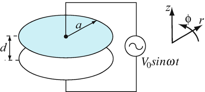
  Figure 12.24

• 12.15 Stored Energy. In a region of space where there are no currents, the time-averaged Poynting vector equals 120 W/m². Assume that this power density is uniform on the surface of a sphere of radius a = 0.1 m, pointing outwards. Calculate the total stored energy in the sphere. The frequency is 1 GHz and the sphere has properties of free space.

12.1.5 Propagation in Lossless, Low-Loss, and Lossy Dielectrics

• 12.16 Energy Density in Dielectrics. A plane wave of given frequency propagates in a perfect dielectric:

  • (a) Calculate the time-averaged stored electric energy density and show that it is equal to the magnetic volume energy density.

  • (b) Suppose now the dielectric is lossy: calculate the time-averaged-stored electric and magnetic energy densities. Are they still the same?

• 12.17 Application: Propagation in Lossy Media. Seawater has a conductivity of 4 S/m. Its permittivity depends on frequency; relative permittivity at 100 Hz is 80, at 100 MHz it is 32, and at 10 GHz it is 24:

  • (a) How can seawater be characterized in terms of its loss at these three frequencies? That is, is seawater a low-loss, high-loss, or a general lossy medium for which no approximations can be made?

  • (b) Calculate the intrinsic impedance at the three frequencies.

  • (c) What can you conclude from these calculations for the propagation properties of seawater?

• 12.18 Generation of a Plane Wave in a Lossy Dielectric. A very thin conducting layer carries a surface current density J₀ [A/m] as shown in Figure 12.25. The frequency is f and the current is directed in the positive z direction. The layer is immersed in seawater, which has permittivity ε, permeability μ₀, and conductivity σ. If the layer is at x = 0, calculate the electric and magnetic fields at x = x₀. Given: J₀ = 1 A/m, f = 100 MHz, σ = 4 S/m, ε₀ = 8.854 × 10⁻¹² F/m, ε_r = 80, μ₀ = 4π × 10⁻⁷ H/m, x₀ = 1 m.

  

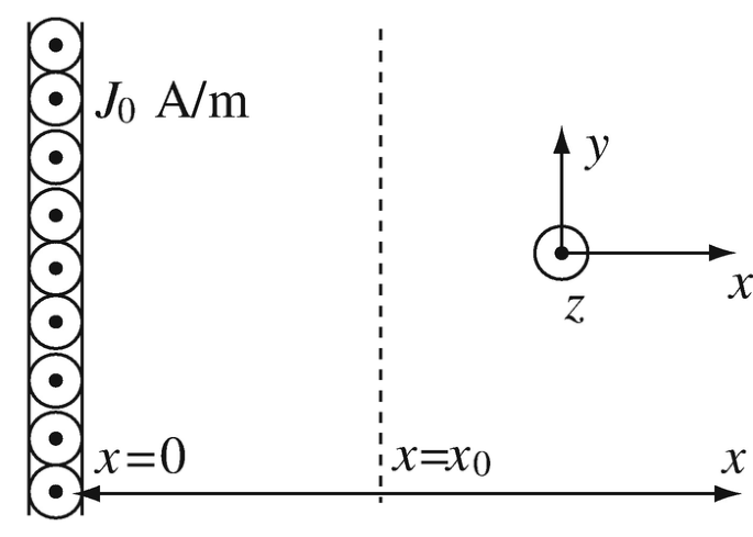
  Figure 12.25

• 12.19 Application: Communication in the Atmosphere. A parabolic antenna of radius b = 1 m transmits at a frequency f = 300 MHz to a receiving antenna a distance d = 200 km away. The receiving antenna is also of radius b and the transmission is parallel to the ground, in the atmosphere, as in Figure 12.26a. Assume that the wave propagates as a plane wave and the beam remains constant in diameter (same diameter as the antennas). Use the following properties: ε = ε₀ [F/m], μ = μ₀ [H/m], σ = 2 × 10⁻⁷ S/m.

  • (a) Calculate the time-averaged power the transmitting antenna must supply if the receiving antenna must receive a magnetic field intensity of magnitude 1 mA/m.

  • (b) In an attempt to reduce the power required, the transmission is directed to a satellite which contains a perfect reflector, as shown in Figure 12.26b. The waves propagate through the atmosphere, into free space to the satellite and back to the receiving antenna. If the satellite is at a height h = 36,000 km and the waves propagate in the atmosphere for a distance q = 20 km in each direction, what is the power needed in this case for the same reception condition as in (a)? Compare the result with that in (a).

    

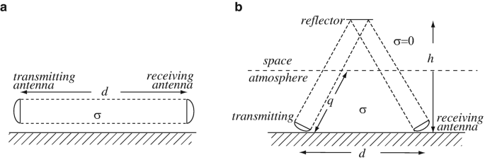
    Figure 12.26

• 12.20 Power Relations in the Atmosphere. A plane wave propagates in the atmosphere. Properties of the atmosphere are ε₀ [F/m], μ₀ [H/m], and σ = 10⁻⁶ S/m. The electric field intensity has an amplitude E₀ =100 V/m in the x direction and E₀ = 100 V/m in the z direction. The frequency of the wave is f = 100 MHz. Find:

  • (a) The direction of propagation.

  • (b) The instantaneous power per unit area in the direction of propagation.

  • (c) The magnitude of the magnetic field intensity after the wave has propagated a distance d = 10 km.

• 12.21 Application: Radar Detection and Ranging of Aircraft. A radar antenna transmits 50 kW at 10 GHz. Assume transmission is in a narrow beam, 1 m² in area, and that within the beam, waves are plane waves. The wave is reflected from an aircraft but only 1% of the power propagates back in the direction of the transmitting antenna. If the airplane is at a distance of 100 km, calculate the total power received by the antenna assuming the reflected power propagates in the same narrow beam as the transmitted power. Assume permittivity and permeability of free space and conductivity of 10⁻⁷ S/m.

• 12.22 Application: Fiber Optics Communication. Two optical fibers are used for communication. One is made of glass with properties μ = μ₀ [H/m] and ε = 1.75ε₀ [F/m] and has an attenuation of 2 dB/km. The second is made of plastic with properties μ = μ₀ and ε = 2.5ε₀ and attenuation of 10 dB/km. Suppose both are used to transmit signals over a length of 10 km. The input to each fiber is a laser, operating at a free-space wavelength of 800 nm and input power of 0.1 W. Calculate:

  • (a) The power available at the end of each fiber.

  • (b) The wavelength, intrinsic (wave) impedance, and phase velocity in each fiber.

  • (c) The phase difference between the two fibers at their ends.

• 12.23 Application: Wave Properties and Remote Sensing in the Atmosphere. A plane wave of frequency f propagates in free space and encounters a large volume of heavy rain. The permittivity of air increases by 8% due to the rain:

  • (a) Calculate the intrinsic impedance, phase constant, and phase velocity in rain and the percentage change in wavelength.

  • (b) Compare the properties calculated in (a) with those in free space. Can any or all of these be used to monitor atmospheric conditions (such as weather prediction)? Explain.

• 12.24 Application: Attenuation in the Atmosphere. Measurements with satellites show that the average solar radiation (solar constant) in space is approximately 1,400 W/m². The total radiation reaching the surface of the Earth on a summer day is approximately 1,100 W/m². 50% of this radiation is in the visible range. To get some insight into the radiation process, assume an atmosphere which is 15 km thick. From this calculate the average attenuation constant in the atmosphere over the visible range assuming it is constant throughout the range and that attenuation is the only loss process.

12.1.6 Propagation in High-Loss Dielectrics and Conductors

• 12.25 Intrinsic Impedance in Copper. Copper has the following properties: μ = μ₀ [H/m], ε = ε₀ [F/m], and σ = 5.7 × 10⁷ S/m. Calculate the intrinsic impedance of copper at 100 MHz:

  • (a) Using the exact formula for general lossy materials.

  • (b) Assuming a high-loss material. Compare with (a) and with the intrinsic impedance of free space.

• 12.26 Application: Communication with Trapped Miners. A serious problem with mine accidents is the difficulty of communicating with trapped miners. The main problem is the lossy nature of soils. Properties of soil depend on composition and moisture but may be approximated as ε_r = 3.2 and σ = 0.02 S/m. Suppose that one wishes to communicate with miners trapped underground by generating a wave at the surface with an electric field intensity of amplitude 400 V/m and a frequency of 300 MHz.

  • (a) If the minimum electric field intensity required at the receiver is 10⁻⁶ V/m, what is the maximum depth of communication possible?

  • (b) Suppose one tries the same at a frequency 10 times higher. What is now the maximum depth?

  • (c) Suppose one tries the same at a frequency 10 times lower. What is now the maximum depth?

  • (d) What is your conclusion from these calculations regarding the possibility of wireless communication with trapped miners?

  Note: There are other effects that limit communication underground, some of which will be discussed in the following chapter including reflections and effects on antennas but these are neglected here.

• 12.27 Skin Depth and Penetration in Lossy Media. Two plane waves propagate in two materials as shown in Figure 12.27:

  • (a) What is the ratio between the distances the waves travel in each material before the electric and magnetic field intensities are attenuated to 1% of their amplitude at the surface? Assume that the waves enter the materials without losses or reflections.

  • (b) What is the ratio between the phase velocities?

    

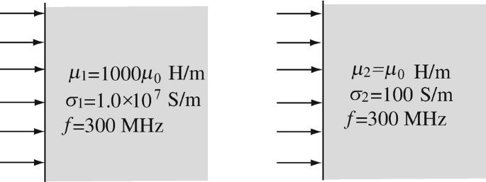
    Figure 12.27

• 12.28 Application: Measurement of Conductivity in Lossy Materials. In an attempt to measure conductivity of a material, a plane wave is applied to one surface of a slab and measured at the other surface. Suppose the electric field intensity just below the left surface of the material is measured as E₀ [V/m]. The electric field intensity at the right surface (again, just below the surface) is 0.1E₀ [V/m]. Permeability and permittivity are those of free space, the material is known to have high conductivity, and the slab is d = 10 mm thick. The measurements are performed at 400 Hz. Calculate the conductivity of the material and its attenuation constant.

• 12.29 Application: Underwater Communication. Suppose a submarine could generate a plane wave and use it to communicate with another submarine in seawater. If the ratio between the amplitude at the receiver and that at the transmitter must be 10⁻¹² or higher, what is the maximum range of communication at:

  • (a) 10 MHz.

  • (b) 100 Hz.

    Assume relative permittivity in both cases is 72 and conductivity of seawater is 4 S/m.

• 12.30 Application: Skin Depth in Conductors. Calculate the skin depth for the following conditions:

  • (a) Copper: f = 10 GHz, μ = μ₀ [H/m], σ = 5.7 × 10⁷ S/m.

  • (b) Mercury: f = 10 GHz, μ = μ₀ [H/m], σ = 1 × 10⁶ S/m.

• 12.31 Wave Impedance in Conductors. Calculate the intrinsic (wave) impedance of copper and iron at 60 Hz and 10 GHz. The conductivity of copper is 5.7 × 10⁷ S/m and that of iron is 1 × 10⁷ S/m. The permeability of copper is μ₀ [H/m] and that of iron is 1,000μ₀ [H/m] at 60 Hz and 2.3μ₀ [H/m] at 10 GHz:

  • (a) Compare these with the wave impedance in free space.

  • (b) What can you conclude from these calculations for the propagation properties of conductors in general and ferromagnetic conductors in particular?

• 12.32 Classification of Lossy Materials. Three materials are considered for their propagation properties: ethanol, concrete and seawater. In ethanol, ε/ε₀ = 24 and σ = 1.3x10⁻⁷ S/m, in concrete, ε/ε₀ = 4.5 and σ = 0.012 S/m and in seawater, ε/ε₀ = 78 and σ = 4 S/m. How do you classify these materials for propagation purposes at 1 MHz and 2.4 GHz assuming properties do not change in the given range of frequencies? Explain.

• 12.33 Application: Skin Depth and Communication in Seawater. How deep does an electromagnetic wave transmitted by a radar operating at 3 GHz propagate in seawater before its amplitude is reduced to 10⁻⁶ of its amplitude just below the surface? Use the following properties: σ = 4 S/m, ε = 76ε₀ [F/m] (at 3 GHz), and μ = μ₀ [H/m]. How good is radar for detection of submarines? Explain.

• 12.34 Penetration of Light in Copper. Since light is an electromagnetic wave and electromagnetic waves penetrate in any material except perfect conductors, calculate the depth of penetration of light into a sheet of copper. The conductivity of copper is 5.7 × 10⁷ S/m, and its permeability is that of free space. Assume the frequency of light (in mid-spectrum) is 5 × 10¹⁴ Hz.

• 12.35 Properties of Seawater at Different Frequencies. The relative permittivity of seawater changes with frequency in a rather complex fashion. A simple approximation is the following: the relative permittivity stays constant at 78 up to 1 GHz. Then it goes down linearly to 5 at 100 GHz and stays constant at a value of 5 above 100 GHz. Its conductivity is 4 S/m and may be assumed frequency independent for the purpose of this problem. Calculate:

  • (a) The approximate range of frequencies over which seawater may be assumed to be a high loss medium, assuming permittivity remains constant.

  • (b) The approximate range of frequencies over which seawater may be assumed to be a low loss medium.

• 12.36 AC Current Distribution in a Conductor. A cable made of iron, with properties as shown in Figure 12.28, carries a current at 100 Hz. If the current density allowed (maximum) is 100 A/mm², find the current density at the center of the conductor (σ = 1 × 10⁷ S/m, μ =20μ₀ [H/m], r = 0.1 m).

  

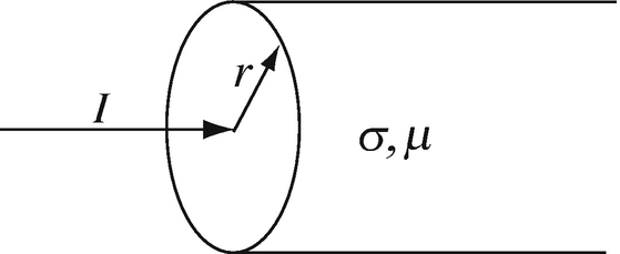
  Figure 12.28

• 12.37 Application: Skin Depth and Design of Cables for AC Power Distribution. A thick wire (cable) is made of steel as shown in Figure 12.29a. If the maximum current density allowed at any point in the material is 10 A/mm²:

  • (a) What is the total current the cable can carry at 60 Hz?

  • (b) To improve the current-carrying capability, a cable is made of 10 thinner wires (see Figure 12.29b) such that the total cross-sectional area is equal to that of the cable in (a). What is the total current the new cable can carry for the same maximum current density, frequency, and material properties?

  • (c) Compare the results in (a) and (b) with the DC current the wire can carry at.

    Note: Assume that the solution for plane waves applies here even though the surface is curved. This is, in general, applicable if the skin depth is small compared to the radius.

    

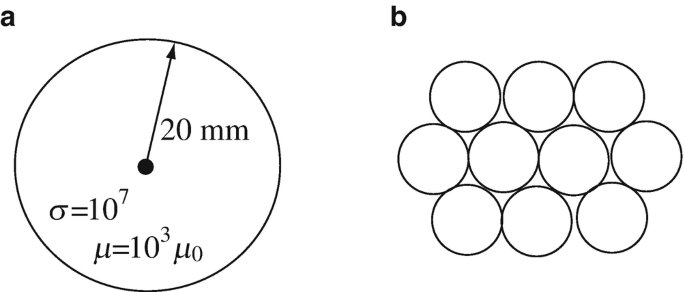
    Figure 12.29

• 12.38 Application: Electromagnetic Shielding. A shielded room is designed to reduce the amplitude of high-frequency waves that penetrate into the room. The shield is made of a nonconducting, nonmagnetic material with a thin coating of conducting material on the outer surface. The shield must reduce the electric field intensity by a factor of 10⁶ compared to the field outside at a frequency of 10 MHz. The conducting layer may be made of aluminum, copper, mu-metal, or a conducting polymer. Conductivities, permeabilities, cost, and mass of the three materials are given in the table below.

  	Cu	Al	Mu-metal	Polymer
  Conductivity [S/m]	5.7 × 107	3.6 × 107	0.5 × 107	0.001
  Permeability [H/m]	μ0	μ0	105μ0	μ0
  Mass [kg/m3]	8,960	2,700	7,800	1,200
  Cost [unit/kg]	1	1.5	100	0.01

  • (a) Calculate the minimum thickness required for each of the four materials.

  • (b) Which material should we choose if the overall important parameter is: 1. Cost. 2. Mass. 3. Volume of conducting material. Use a unit area of the wall for comparison.

12.1.7 Dispersion and Group Velocity

• 12.39 Dispersion and Group Velocity. Under certain conditions, a wave propagates with the following phase constant:

  $$ \beta =\omega \sqrt{\mu \varepsilon}\sqrt{1-\frac{\omega_c^2}{\omega^2}}\kern1em \left[\frac{\mathrm{rad}}{\mathrm{m}}\right] $$

  where ω [rad/s] is the angular frequency of the wave, and ω_c [rad/s] is a fixed angular frequency. Because this gives the relation between β and ω, it is a dispersion relation:

  • (a) Plot the dispersion relation for the wave: use ω_c = 10⁷, 10⁷ ≤ ω ≤ 2 × 10⁷ [rad/s].

  • (b) What are the phase and group velocities?

  • (c) What happens at ω = ω_c? Explain.

• 12.40 Dispersion and Group Velocity. The dispersion relation for a wave is given as

  $$ \beta =\sqrt{\omega^2\mu \varepsilon -\frac{\pi^2}{a}}\kern1em \left[\frac{\mathrm{rad}}{\mathrm{m}}\right] $$

  • (a) Plot the dispersion relation. a is a constant and π²/a < ω²με.

  • (b) Find the group and phase velocities.

• 12.41 Phase and Group Velocities. Show that the following relation between group and phase velocity exists:

  $$ {v}_g={v}_p+\beta \frac{{d v}_p}{d\beta}\kern1em \left[\frac{\mathrm{m}}{\mathrm{s}}\right] $$

• 12.42 Phase and Group Velocities in Lossy Dielectrics. A plane wave with electric field intenstity E = $\hat{\mathbf{x}}100{e}^{-j2z}\left[\mathrm{V}/\mathrm{m}\right]$ propagates in rubber, which has properties μ = μ₀ [H/m], ε = 4ε₀ [F/m], and σ = 0.001 S/m and may be considered to be a very low-loss dielectric. Calculate:

  • (a) The phase velocity in the material.

  • (b) The group velocity in the material.

  • (c) The energy transport velocity.

  • (d) What is the conclusion from the results in (a)–(c)?

• 12.43 Group Velocity and Dispersion in Low-Loss Media. A general low-loss medium is given in which the term σ/ωε is small but not negligible:

  • (a) Calculate the group velocity.

  • (b) Plot the group velocity as a function of frequency.

  • (c) Is the medium dispersive and, if so, is the dispersion normal or anomalous? Explain.

12.1.8 Polarization of Plane Waves

• 12.44 Polarization of Plane Waves. The magnetic field intensity of a plane wave is given as $\mathbf{H}(x)=\hat{\mathbf{y}}10{e}^{- j\beta x}$ [A/m]. What is the polarization of this wave?

• 12.45 Polarization of Plane Waves. The magnetic field intensity of a plane wave is given as $\mathbf{H}(x)=\hat{\mathbf{y}}10{e}^{- j\beta x}+\hat{\mathbf{z}}15{e}^{- j\beta x}\;\left[\mathrm{A}/\mathrm{m}\right]$. What is the polarization of this wave?

• 12.46 Polarization of Plane Waves. The electric field intensity of a plane wave is given as $\mathbf{E}(x)=\hat{\mathbf{y}}10{e}^{-0.1x}\left({e}^{- j\beta x}+{e}^{j\beta x}\right)+\hat{\mathbf{y}}10{e}^{-0.1x}\left({e}^{- j\beta x}-{e}^{j\beta x}\right)\;\left[\mathrm{V}/\mathrm{m}\right]$. What is the polarization of this wave?

• 12.47 Polarization of Plane Waves. The electric field intensity of a plane wave is given as $\mathbf{E}\left(x, t\right)=\hat{\mathbf{y}}100\cos \left(\omega t-\beta x\right)+\hat{\mathbf{z}}200\cos \left(\omega t-\beta x-\pi /2\right)$ [V/m]. What is the polarization of this wave?

• 12.48 Polarization of Superposed Plane Waves. Two plane waves propagate in the same direction. Both waves are at the same frequency and have equal amplitudes. Wave A is polarized linearly in the x direction, and wave B is polarized in the direction of $\hat{\mathbf{x}}+\hat{\mathbf{y}}$. In addition, wave B lags behind wave A by a small angle θ. What is the polarization of the sum of the two waves?

• 12.49 Polarization of Plane Waves. The magnetic field intensity of a plane wave is given as $\mathbf{H}\left(x, t\right)=\hat{\mathbf{y}}100\kern-0.1em \cos \kern-0.15em \left(\omega t-\beta x\right)+\hat{\mathbf{z}}200\cos \left(\omega t-\beta x+\pi /2\right)$ [A/m]. What is the polarization of this wave?