Maxwell’s Equations

Abstract

Most students in engineering and science have heard the term “Maxwell’s equations,” and some may also have heard that Maxwell’s equations “describe all electromagnetic phenomena.” However, it is not always clear what exactly do we mean by these equations. How are they any different from what we have studied in the previous chapters? We recall discussing static and time-dependent fields and, in the process, discussed many applications. To do so, we used the definitions of the curl and divergence of the electric and magnetic fields: what we called “the postulates.” Are Maxwell’s equations different? Do they add anything to the previously described phenomena? Perhaps the best question to ask is the following: Is there any other electromagnetic phenomenon that was not discussed in the previous chapters because the definitions we used were not sufficient to do so? If so, do Maxwell’s equations define these yet unknown properties of the electromagnetic field? The answer to the latter is emphatically yes.

From a long view of the history of mankind—seen from say, ten thousand years from now—there can be little doubt that the most significant event of the 19th century will be judged as Maxwell’s discovery of the laws of electrodynamics. The American civil war will pale into provincial insignificance in comparison with this important scientific event of the same decade.

Richard P. Feynman (1918–1988)

Physicist, Nobel laureate

Problems

11.1.1 Maxwell’s Equations, Displacement Current, and Continuity

• 11.1 Displacement Current Density. A magnetic flux density, B = ŷ(0.1cos5z)cos100t [T] exists in a linear, isotropic, homogeneous material characterized by ε and μ. Find the displacement current density in the material if there are no source charges or current densities in the material.

• 11.2 Displacement Current in Spherical Capacitor. Determine the displacement current I_d [A] which flows between two concentric, conducting spherical shells of radii a and b [m] where b > a in free space with a voltage difference V₀sinωt [V] applied between the spheres.

• 11.3 Application: Displacement Current in Cylindrical Capacitor. A voltage source V₀sinωt [V] is connected between two concentric conductive cylinders of radii r = a and r = b [m], where b > a, with length L [m]. ε = ε_rε₀ [F/m], μ = μ₀ [H/m], and σ = 0 for a < r < b. Neglect any end effects and find:

  • (a) The displacement current density at any point a < r < b.

  • (b) The total displacement current I_d flowing between the two cylinders.

• 11.4 Conservation of Charge and Displacement Current. Show that the displacement current density in Maxwell’s second equation (Ampère’s law) is a direct consequence of the law of conservation of charge.

• 11.5 Application: Displacement and Conduction Current Densities in Lossy Capacitor. A lossy dielectric is located between two parallel plates which are connected to an AC source (Figure 11.5). Material properties of the dielectric are ε = 9ε₀ [F/m], μ = μ₀ [H/m], and σ = 4 S/m. The source is given as V = 1cosωt [V]. Calculate the frequency at which the magnitude of the displacement current density is equal to the magnitude of the conduction current density. Assume all material properties are independent of frequency.

  

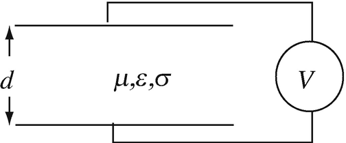
  Figure 11.5

• 11.6 Application: Displacement and Conduction Current Densities. A capacitor is made of two parallel plates with a dielectric between them. The area of each plate is A [m²] and the dielectric is d [m] thick. The dielectric is lossy with a permittivity ε [F/m] and conductivity σ [S/m]. If the capacitor is connected to a sinusoidal AC source of amplitude V [V] and angular frequency ω [rad/s]:

  • (a) Find the ratio between the amplitudes of the conduction current density and displacement current density.

  • (b) Show that the conduction and displacement current densities are 90° out of phase.

• 11.7 Application: Lossy Capacitor. The capacitor in Problem 11.6 is connected to a 12 V DC source and charged for a long period of time. Now the source is disconnected. Find the time constant of discharge of the capacitor.

• 11.8. Application: Displacement Current. An AC generator operating at a frequency of 1 GHz is connected with a wire to a small conducting sphere of radius a = 10 mm at some distance away (see Figure 11.6). If the sphere is in free space, calculate the current in the wire. Neglect any effect the ground may have. The generator generates a sinusoidal voltage of amplitude 100 V.

  

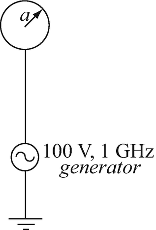
  Figure 11.6

• 11.9 Application: Displacement current. Two conducting spheres, each of radius a = 0.2 m are connected to an AC source of amplitude 120 V and frequency of 100 kHz as shown in Figure 11.7, separated a distance d = 10 m apart. Assume the voltage source is sinusoidal (V(t) = 120sin2πft) and free space everywhere. Calculate the current supplied by the source. Hint: think about the spheres as forming a capacitor and assume charge on the spheres at any instant in time is uniformly distributed on their surfaces.

  

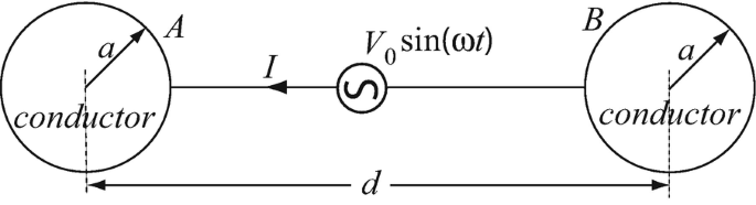
  Figure 11.7

11.1.2 Maxwell’s Equations

• 11.10 Maxwell’s Equations. An electric field intensity and a magnetic field intensity are given as follows:

  $$ {\displaystyle \begin{array}{l}\mathbf{E}=\hat{\mathbf{y}}\kern-1pt 120\pi \cos \left({10}^6\pi t+\beta z\right)\kern1em \left[\mathrm{V}/\mathrm{m}\right]\\ {}\mathbf{H}=\hat{\mathbf{x}}{H}_0\cos \left({10}^6\pi t+\beta z\right)\kern1em \left[\mathrm{A}/\mathrm{m}\right]\end{array}} $$

  • (a) What values of H₀ and β are required for the two fields to satisfy Maxwell’s equations in free space?

  • (b) What values of H₀ and β are required for the two fields to satisfy Maxwell’s equations in a perfect dielectric with relative permittivity 4 and relative permeability 1? Assume there are no charge densities in the dielectric.

• 11.11 Dependency in Maxwell’s Equations. Show that Eq. (11.8) (∇ ⋅ B = 0) can be derived from Eq. (11.5) and, therefore, is not an independent equation.

• 11.12 Dependency in Maxwell’s Equations. Show that Eq. (11.7) (∇ ⋅ D = ρ_v) can be derived from Eq. (11.6) with the use of the continuity equation [Eq. (11.13)] and, therefore, is not an independent equation.

• 11.13 The Lorenz Condition (Gauge). Show that the Lorenz condition in Eq. (11.49) leads to the continuity equation. Hint: Use the expression for electric potential due to a general volume charge distribution and the expression for the magnetic vector potential due to a general current density in a volume.

• 11.14 Application: Displacement Current in a Conductor. A copper wire with conductivity σ = 5.7 × 10⁷ S/m carries a sinusoidal current of amplitude I₀ = 0.1 A and frequency f = 100 MHz. Assume the current is uniformly distributed within the conductor’s cross-section. Calculate the amplitude of the displacement current in the wire.

• 11.15 Maxwell’s Equations in Cylindrical Coordinates. Write Maxwell’s equations explicitly in cylindrical coordinates by expanding the expressions in Eqs. (11.24) through (11.27).

• 11.16 Maxwell’s Equations. A time-dependent magnetic field is given as $\mathbf{B}=\hat{\mathbf{x}}20{e}^{j\left({10}^4t+{10}^{-4}z\right)}\;\left[\mathrm{T}\right]$ in a material with properties ε_r = 9 and μ_r = 1. Assume there are no sources in the material. Using Maxwell’s equations:

  • (a) Calculate the electric field intensity in the material.

  • (b) Calculate the electric flux density and the magnetic field intensity in the material.

• 11.17 Maxwell’s Equations. A time-dependent electric field intensity is given as $\mathbf{E}=\hat{\mathbf{x}}\kern-1pt 10\pi \cos \left({10}^6t-50z\right)\ \left[\mathrm{V}/\mathrm{m}\right]$. The field exists in a material with properties ε_r = 4 and μ_r = 1. Given that J = 0 and ρ_v = 0, calculate the magnetic field intensity and magnetic flux density in the material.

11.1.3 Potential Functions

• 11.18 Current Density as a Primary Variable in Maxwell’s Equations. Given Maxwell’s equations in a linear, isotropic, homogeneous medium. Assume that there are no source current densities and no charge densities anywhere in the solution space. An induced current density J_e [A/m²] exists in conducting materials. Assume the whole space is conducting, with a very low conductivity, σ [S/m]. Rewrite Maxwell’s equations in terms of the current density J_e = σE. In other words, assume you need to solve for J_e directly.

• 11.19 Magnetic Scalar Potential. Write an equation, equivalent to Maxwell’s equations in terms of a magnetic scalar potential in a linear, isotropic, homogeneous medium. State the conditions under which this can be done:

  • (a) Show that Maxwell’s equations reduce to a second-order partial differential equation in the scalar potential. What are the assumptions necessary for this equation to be correct?

  • (b) What can you say about the relation between the electric and magnetic field intensities under the given conditions?

• 11.20 Magnetic Vector Potential. Given: Maxwell’s equations and the vector B = ∇ × A, in a linear, isotropic, homogeneous medium. Assume that E = 0 for static fields:

  • (a) By neglecting the displacement currents, show that Maxwell’s equations reduce to a second-order partial differential equation in A alone.

  • (b) What is the electric field intensity?

  • (c) Show that by using the Coulomb’s gauge, the equation in (a) becomes a simple Poisson equation.

• 11.21 An Electric Vector Potential. A vector potential may be derived as ∇ × F = –D where D is the electric flux density:

  • (a) What must be the static magnetic field intensity (other than H = 0 or H = C, where C is a constant vector) if we know that in the static case, ∇ × H = 0?

  • (b) Find a representation of Maxwell’s equations in terms of the vector potential F in a current-free region (i.e., a region without source currents).

  • (c) What might the divergence of F be for the representation in (b) to be useful? Explain.

• 11.22 Modified Vector Potential. A modified vector potential may be defined as F = A + ∇ψ, where A is the magnetic vector potential as defined in Eq. (11.40) and ψ is any scalar function:

  • (a) Show that this is a correct definition of the vector potential.

  • (b) Find an expression of Maxwell’s equations in terms of F alone.

  • (c) How would you name the two potentials F and ψ?

• 11.23 The Hertz Potential. In a linear, isotropic, homogeneous medium devoid of sources, one can derive the fields from a single potential called the Hertz potential, π, as follows:

  $$ \mathbf{A}= j\omega \mu \varepsilon \boldsymbol{\uppi}, \kern1.25em V=-\nabla \cdot \boldsymbol{\uppi} $$

  where A is the magnetic vector potential and V the electric scalar potential.

  Find the expressions for the electric and magnetic field intensities to show that they are dependent on π alone.

• 11.24 The Use of a Gauge. In a linear, isotropic, homogeneous medium devoid of sources, one can define the magnetic Hertz potential π_m as

  $$ \mathbf{E}=- j\omega \mu \nabla \times {\boldsymbol{\uppi}}_m\kern1em \left[\mathrm{V}/\mathrm{m}\right] $$

  Show that one can write Maxwell’s equations in the frequency domain in terms of π_m alone provided a proper gauge is defined. What is that gauge?

11.1.4 Interface Conditions for General Fields

• 11.25 Application: Displacement Current Density in a Dielectric. A time-dependent electric field intensity is applied on a dielectric as shown in Figure 11.8. The electric field intensity in free space is given as $\mathbf{E}=\hat{\mathbf{z}}{E}_0\cos \omega t\ \left[\mathrm{V}/\mathrm{m}\right]$. The relative permittivity of the material is ε_r = 25. For E₀ = 100 V/m and ω = 10⁹ rad/s, calculate the peak displacement current density in the dielectric (there are no surface charges at the interface between air and material).

  

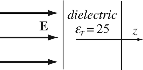
  Figure 11.8

• 11.26 Interface Conditions for General Materials. Two dielectrics meet at an interface (see Figure 11.9) at x = 0. A sinusoidal electric field intensity of peak value 80 V/m and frequency 1 kHz exists in dielectric (1) directed as shown. For x < 0, ε = 2ε₀ [F/m], and μ = μ₀ [H/m]. For x > 0, ε = 3ε₀, and μ = 2μ₀. If the electric field intensity vector is incident at 30° from the normal, find the magnitudes of the electric field intensity and the electric flux density on each side of the interface if:

  • (a) There is no charge density on the interface.

  • (b) A charge density of magnitude 0.6 nC/m² exists on the interface and the electric field intensity in medium (1) is the same as in (a). The charge density varies with time exactly the same as the electric field intensity.

  

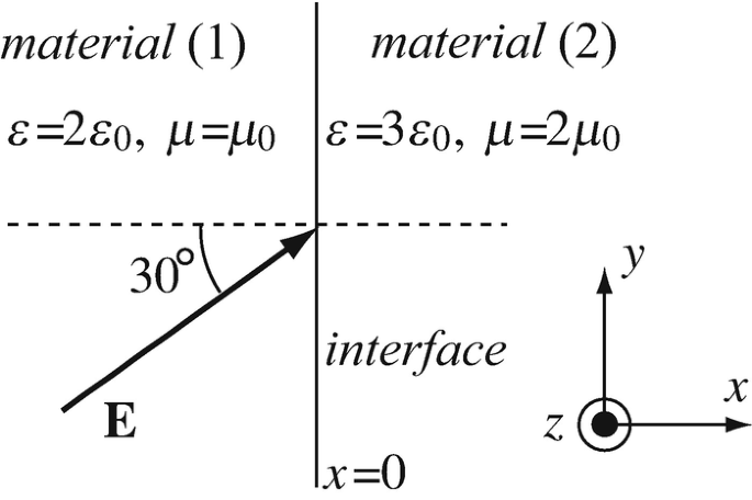
  Figure 11.9

• 11.27 Calculation of Fields Across Interfaces. A region, denoted as region (1), occupies the space x < 0 and has relative permeability μ_r1 = 6. The magnetic field intensity in region (1) is ${\mathbf{H}}_1=\hat{\mathbf{x}}4+\hat{\mathbf{y}}-\hat{\mathbf{z}}2$ [A/m]. Region (2) is defined as x > 0 with μ_r2 = 5.0. No current exists at the interface. Find B in region (2).

• 11.28 Interface Conditions for Permeable Materials. An interface between free space and a perfectly permeable material exists. In free space (1), μ = μ₀ [H/m], ε = ε₀ [F/m], and σ =0. In the permeable material (2), μ = ∞, σ = 0, and ε = ε₀. Define the interface conditions at the interface between the two materials.

• 11.29 Surface Current Density at Interfaces. Two materials meet at an interface as shown in Figure 11.10. Material (1) has relative permeability 4 and material (2) has relative permeability 50. The interface is at z = 0. The magnetic flux density in material (1) is given as $\mathbf{B}=\hat{\mathbf{x}}0.01+\hat{\mathbf{y}}0.02+\hat{\mathbf{z}}0.015\ \left[\mathrm{T}\right]$. In material (2), it is known that all tangential components of H are zero. It is assumed that material (2) is conducting.

  • (a) Calculate the surface current density that must exist on the interface for this condition to be satisfied.

  • (b) Calculate the magnetic flux density in material (2).

    

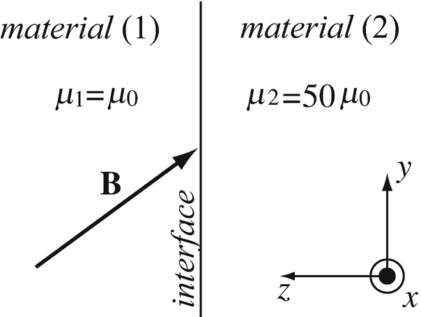
    Figure 11.10

• 11.30 Surface Current Density at an Interface. The interface between a conducting medium and free space coincides with the x–y plane. The conducting medium occupies the space z > 0 and has permeability μ₀ [H/m]. The magnetic field intensity in free space is given as $\mathbf{H}=\hat{\mathbf{x}}\kern-1pt {10}^5+\hat{\mathbf{y}}2\times {10}^5+\hat{\mathbf{z}}\kern-0.75pt {10}^4$ [A/m].

  • (a) The magnetic field intensity in the conducting medium.

  • (b) The surface current density that must exist on the interface required to cancel the tangential components of the magnetic field intensity in the conductor.

11.1.5 Time-Harmonic Equations/Phasors

• 11.31 Vector Operations on Phasors. Two complex vectors are given as A = a + jb and B = c + jd, where a, b, c, and d are real vectors. Calculate (^* indicates complex conjugate) and compare the following products:

  $$ {\displaystyle \begin{array}{cccc}\mathbf{A}\cdot \mathbf{A}& \mathbf{A}\cdot {\mathbf{A}}^{\ast }& \mathbf{A}\cdot \mathbf{B}& \mathbf{A}\cdot {\mathbf{B}}^{\ast}\kern1em {\mathbf{A}}^{\ast}\cdot \mathbf{B}\\ {}\mathbf{A}\times \mathbf{A}& \mathbf{A}\times {\mathbf{A}}^{\ast }& \mathbf{A}\times \mathbf{B}& \mathbf{A}\times {\mathbf{B}}^{\ast}\kern0.75em {\mathbf{A}}^{\ast}\times \mathbf{B}\end{array}} $$
  $$ \mathbf{B}\times \mathbf{A}\kern1em \mathbf{B}\times {\mathbf{A}}^{\ast}\kern1em {\mathbf{B}}^{\ast}\times \mathbf{A} $$

• 11.32 Conversion of Phasors to the Time Domain. A magnetic field intensity is given as $\mathbf{H}=\hat{\mathbf{y}}5{e}^{- j\beta z}$ [A/m]. Write the time-dependent magnetic field intensity.

• 11.33 Conversion to Phasors. The following magnetic field intensity is given in a domain 0 ≤ x ≤ a, 0 ≤ y ≤ b:

  $$ H\left(x, y, z, t\right)={H}_0\kern-0.15em \sin \frac{m\pi x}{a}\cos \frac{n\pi y}{b}\cos \left(\omega t- kz\right)\kern1em \left[\mathrm{A}/\mathrm{m}\right] $$

  where x, y, and z are the space variables, m and n are integers, and k is a constant. Find the rectangular, polar, and exponential phasor representations of the field.

• 11.34 Conversion to Phasors. An electric field intensity is given as

  $$ E\left(z, t\right)={E}_1\cos \left(\omega t- kz+\psi \right)+{E}_2\cos \left(\omega t+ kz+\psi \right)\kern1em \left[\mathrm{V}/\mathrm{m}\right] $$

  Write the phasor form of E in polar and exponential forms.

• 11.35 Conversion of Phasors to the Time Domain. A phasor is given as

  $$ E\left(x, z\right)={E}_0{e}^{-j{\beta}_0\left(x\kern-0.1em \sin \kern-0.11em {\theta}_i+z\kern-0.1em \cos \kern-0.11em {\theta}_i\right)}\kern1em \left[\mathrm{V}/\mathrm{m}\right] $$

  where x and z are variables and β₀ and θ_i are constants. Find the time-dependent form of the field E.

• 11.36 Conversion to Phasors. The electric field intensity in a domain is given as

  $$ {E}_x\left(z, t\right)={E}_0\cos \left(\omega t- kz+\phi \right)\kern1em \left[\mathrm{V}/\mathrm{m}\right] $$

  Find:

  • (a) The phasor representation of the field in exponential form.

  • (b) The first-order time derivative of the phasor.

• 11.37 Time-Harmonic Fields. The electric field intensity

  $$ \mathbf{E}=\hat{\mathbf{x}}10\pi \cos \left({10}^6t-50z\right)+\hat{\mathbf{y}}10\pi \cos \left({10}^6t-50z\right)\kern1em \left[\mathrm{V}/\mathrm{m}\right] $$

  is given in a linear, isotropic, homogeneous medium of permeability μ₀ [H/m] and permittivity ε₀ [F/m]. Write the magnetic field intensity and the magnetic flux density:

  • (a) In terms of the time-dependent electric field intensity.

  • (b) In terms of the time-harmonic electric field intensity.

• 11.38 Time-Harmonic Fields. The magnetic field intensity in air is given as $\mathbf{H}=\left(\hat{\mathbf{x}}{H}_x+\hat{\mathbf{y}}{H}_y+\hat{\mathbf{z}}{H}_z\right){e}^{j\beta z}{e}^{j\phi}$ [A/m], where H_x, H_y and H_z are complex numbers given as H_x = h_x + jg_x, H_y = h_y + jg_y and H_z = h_z + jg_z:

  • (a) What is the time-dependent magnetic field intensity H in air?

  • (b) Write the magnetic field intensity in terms of amplitude and phase.

• 11.39 Conversion of Phasors. Two vector fields are given in phasor form as

  $$ {\mathbf{E}}_1=\hat{\mathbf{x}}\left(20+j20\right){e}^{j0.3\pi z}+\hat{\mathbf{y}}\left(10-j20\right){e}^{j0.3\pi z},\kern1em {\mathbf{E}}_2=-\hat{\mathbf{x}}\left(20-j10\right){e}^{j0.3\pi z}+\hat{\mathbf{y}}\left(20+j20\right){e}^{j0.3\pi z}\kern1em \left[\mathrm{V}/\mathrm{m}\right] $$

  Calculate:

  • (a) The time domain representation of the two fields.

  • (b) The sum E₁ + E₂ in phasor form and in the time domain.

  • (c) The difference E₁ – E₂ in phasor form and in the time domain.

  • (d) The vector product of the two fields in the time domain and in phasor form.

  • (e) The scalar product of the two fields in the time domain and in phasor form.