Programming for GPUs

Abstract

Over the last few decades, Graphics Processing Units (GPUs) have evolved from specialized hardware devices capable of drawing images on a screen to general-purpose devices capable of executing complex parallel kernels. Nowadays, nearly every computer includes a GPU alongside a traditional CPU, and many programs may be accelerated by offloading part of a parallel algorithm from the CPU to the GPU.

Over the last few decades, Graphics Processing Units (GPUs) have evolved from specialized hardware devices capable of drawing images on a screen to general-purpose devices capable of executing complex parallel kernels. Nowadays, nearly every computer includes a GPU alongside a traditional CPU, and many programs may be accelerated by offloading part of a parallel algorithm from the CPU to the GPU.

In this chapter, we will describe how a typical GPU works, how GPU software and hardware execute a SYCL application, and tips and techniques to keep in mind when we are writing and optimizing parallel kernels for a GPU.

Performance Caveats

As with any processor type, GPUs differ from vendor to vendor or even from product generation to product generation; therefore, best practices for one device may not be best practices for a different device. The advice in this chapter is likely to benefit many GPUs, both now and in the future, but…

To achieve optimal performance for a particular GPU, always consult the GPU vendor’s documentation!

Links to documentation from many GPU vendors are provided at the end of this chapter.

How GPUs Work

This section describes how typical GPUs work and how GPUs differ from other accelerator types.

GPU Building Blocks

Figure 15-1 shows a very simplified GPU consisting of three high-level building blocks:

• 1. Execution resources: A GPU’s execution resources are the processors that perform computational work. Different GPU vendors use different names for their execution resources, but all modern GPUs consist of multiple programmable processors. The processors may be heterogeneous and specialized for particular tasks, or they may be homogeneous and interchangeable. Processors for most modern GPUs are homogeneous and interchangeable.

• 2. Fixed functions: GPU fixed functions are hardware units that are less programmable than the execution resources and are specialized for a single task. When a GPU is used for graphics, many parts of the graphics pipeline such as rasterization or raytracing are performed using fixed functions to improve power efficiency and performance. When a GPU is used for data-parallel computation, fixed functions may be used for tasks such as workload scheduling, texture sampling, and dependence tracking.

• 3. Caches and memory: Like other processor types, GPUs frequently have caches to store data accessed by the execution resources. GPU caches may be implicit, in which case they require no action from the programmer, or may be explicit scratchpad memories, in which case a programmer must purposefully move data into a cache before using it. Many GPUs also have a large pool of memory to provide fast access to data used by the execution resources.

  Figure 15-1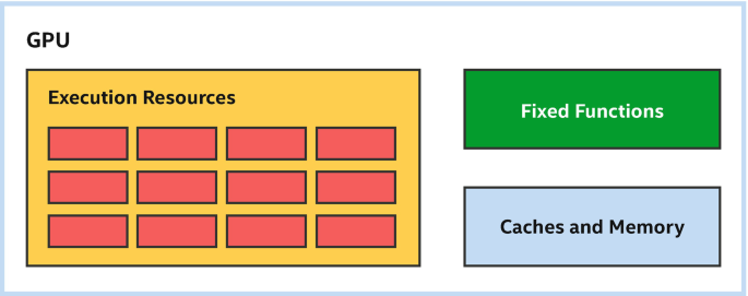

  

  Typical GPU building blocks—not to scale!

Simpler Processors (but More of Them)

Traditionally, when performing graphics operations, GPUs process large batches of data. For example, a typical game frame or rendering workload involves thousands of vertices that produce millions of pixels per frame. To maintain interactive frame rates, these large batches of data must be processed as quickly as possible.

A typical GPU design tradeoff is to eliminate features from the processors forming the execution resources that accelerate single-threaded performance and to use these savings to build additional processors, as shown in Figure 15-2. For example, GPU processors may not include sophisticated out-of-order execution capabilities or branch prediction logic used by other types of processors. Due to these tradeoffs, a single data element may be processed on a GPU slower than it would on another processor, but the larger number of processors enables GPUs to process many data elements quickly and efficiently.

Figure 15-2

GPU processors are simpler, but there are more of them

To take advantage of this tradeoff when executing kernels, it is important to give the GPU a sufficiently large range of data elements to process. To demonstrate the importance of offloading a large range of data, consider the matrix multiplication kernel we have been developing and modifying throughout this book.

A REMINDER ABOUT MATRIX MULTIPLICATION

In this book, matrix multiplication kernels are used to demonstrate how changes in a kernel or the way it is dispatched affects performance. Although matrix multiplication performance are significantly improved using the techniques described in this chapter, matrix multiplication is such an important and common operation that many hardware (GPU, CPU, FPGA, DSP, etc.) vendors have implemented highly tuned versions of many routines including matrix multiplication. Such vendors invest significant time and effort implementing and validating functions for specific devices and in some cases may use functionality or techniques that are difficult or impossible to use in standard kernels.

USE VENDOR-PROVIDED LIBRARIES!

When a vendor provides a library implementation of a function, it is almost always beneficial to use it rather than re-implementing the function as a kernel! For matrix multiplication, one can look to oneMKL as part of Intel’s oneAPI toolkits for solutions appropriate for DPC++ programmers.

A matrix multiplication kernel may be trivially executed on a GPU by submitting it into a queue as a single task. The body of this matrix multiplication kernel looks exactly like a function that executes on the host CPU and is shown in Figure 15-3.

Figure 15-3

A single task matrix multiplication looks a lot like CPU host code

If we try to execute this kernel on a CPU, it will probably perform okay—not great, since it is not expected to utilize any parallel capabilities of the CPU, but potentially good enough for small matrix sizes. As shown in Figure 15-4, if we try to execute this kernel on a GPU, however, it will likely perform very poorly, because the single task will only utilize a single GPU processor.

Figure 15-4

A single task kernel on a GPU leaves many execution resources idle

Expressing Parallelism

To improve the performance of this kernel for both CPUs and GPUs, we can instead submit a range of data elements to process in parallel, by converting one of the loops to a parallel_for. For the matrix multiplication kernel, we can choose to submit a range of data elements representing either of the two outermost loops. In Figure 15-5, we’ve chosen to process rows of the result matrix in parallel.

Figure 15-5

Somewhat-parallel matrix multiplication

CHOOSING HOW TO PARALLELIZE

Choosing which dimension to parallelize is one very important way to tune an application for both GPUs and other device types. Subsequent sections in this chapter will describe some of the reasons why parallelizing in one dimension may perform better than parallelizing in a different dimension.

Even though the somewhat-parallel kernel is very similar to the single task kernel, it should run better on a CPU and much better on a GPU. As shown in Figure 15-6, the parallel_for enables work-items representing rows of the result matrix to be processed on multiple processor resources in parallel, so all execution resources stay busy.

Figure 15-6

Somewhat-parallel kernel keeps more processor resources busy

Note that the exact way that the rows are partitioned and assigned to different processor resources is not specified, giving an implementation flexibility to choose how best to execute the kernel on a device. For example, instead of executing individual rows on a processor, an implementation may choose to execute consecutive rows on the same processor to gain locality benefits.

Expressing More Parallelism

We can parallelize the matrix multiplication kernel even more by choosing to process both outer loops in parallel. Because parallel_for can express parallel loops over up to three dimensions, this is straightforward, as shown in Figure 15-7. In Figure 15-7, note that both the range passed to parallel_for and the item representing the index in the parallel execution space are now two-dimensional.

Figure 15-7

Even more parallel matrix multiplication

Exposing additional parallelism will likely improve the performance of the matrix multiplication kernel when run on a GPU. This is likely to be true even when the number of matrix rows exceeds the number of GPU processors. The next few sections describe possible reasons why this may be the case.

Simplified Control Logic (SIMD Instructions)

Many GPU processors optimize control logic by leveraging the fact that most data elements tend to take the same control flow path through a kernel. For example, in the matrix multiplication kernel, each data element executes the innermost loop the same number of times since the loop bounds are invariant.

When data elements take the same control flow path through a kernel, a processor may reduce the costs of managing an instruction stream by sharing control logic among multiple data elements and executing them as a group. One way to do this is to implement a Single Instruction, Multiple Data or SIMD instruction set, where multiple data elements are processed simultaneously by a single instruction.

THREADS VS. INSTRUCTION STREAMS

In many parallel programming contexts and GPU literature, the term “thread” is used to mean an “instruction stream.” In these contexts, a “thread” is different than a traditional operating system thread and is typically much more lightweight. This isn’t always the case, though, and in some cases, a “thread” is used to describe something completely different.

Since the term “thread” is overloaded and easily misunderstood, this chapter uses the term “instruction stream” instead.

Figure 15-8

Four-wide SIMD processor: The four ALUs share fetch/decode logic

The number of data elements that are processed simultaneously by a single instruction is sometimes referred to as the SIMD width of the instruction or the processor executing the instruction. In Figure 15-8, four ALUs share the same control logic, so this may be described as a four-wide SIMD processor.

GPU processors are not the only processors that implement SIMD instruction sets . Other processor types also implement SIMD instruction sets to improve efficiency when processing large sets of data. The main difference between GPU processors and other processor types is that GPU processors rely on executing multiple data elements in parallel to achieve good performance and that GPU processors may support wider SIMD widths than other processor types. For example, it is not uncommon for GPU processors to support SIMD widths of 16, 32, or more data elements.

PROGRAMMING MODELS: SPMD AND SIMD

Although GPU processors implement SIMD instruction sets with varying widths, this is usually an implementation detail and is transparent to the application executing data-parallel kernels on the GPU processor. This is because many GPU compilers and runtime APIs implement a Single Program, Multiple Data or SPMD programming model, where the GPU compiler and runtime API determine the most efficient group of data elements to process with a SIMD instruction stream, rather than expressing the SIMD instructions explicitly. The “Sub-Groups” section of Chapter 9 explores cases where the grouping of data elements is visible to applications.

In Figure 15-9, we have widened each of our execution resources to support four-wide SIMD, allowing us to process four times as many matrix rows in parallel.

Figure 15-9

Executing a somewhat-parallel kernel on SIMD processors

The use of SIMD instructions that process multiple data elements in parallel is one of the ways that the performance of the parallel matrix multiplication kernels in Figures 15-5 and 15-7 is able to scale beyond the number of processors alone. The use of SIMD instructions also provides natural locality benefits in many cases, including matrix multiplication, by executing consecutive data elements on the same processor.

Kernels benefit from parallelism across processors and parallelism within processors!

Predication and Masking

Sharing an instruction stream among multiple data elements works well so long as all data elements take the same path through conditional code in a kernel. When data elements take different paths through conditional code, control flow is said to diverge. When control flow diverges in a SIMD instruction stream, usually both control flow paths are executed, with some channels masked off or predicated. This ensures correct behavior, but the correctness comes at a performance cost since channels that are masked do not perform useful work.

To show how predication and masking works, consider the kernel in Figure 15-10, which multiplies each data element with an “odd” index by two and increments each data element with an “even” index by one.

Figure 15-10

Kernel with divergent control flow

Let’s say that we execute this kernel on the four-wide SIMD processor shown in Figure 15-8 and that we execute the first four data elements in one SIMD instruction stream and the next four data elements in a different SIMD instruction stream and so on. Figure 15-11 shows one of the ways channels may be masked and execution may be predicated to correctly execute this kernel with divergent control flow.

Figure 15-11

Possible channel masks for a divergent kernel

SIMD Efficiency

SIMD efficiency measures how well a SIMD instruction stream performs compared to equivalent scalar instruction streams. In Figure 15-11, since control flow partitioned the channels into two equal groups, each instruction in the divergent control flow executes with half efficiency. In a worst-case scenario, for highly divergent kernels, efficiency may be reduced by a factor of the processor’s SIMD width.

All processors that implement a SIMD instruction set will suffer from divergence penalties that affect SIMD efficiency, but because GPU processors typically support wider SIMD widths than other processor types, restructuring an algorithm to minimize divergent control flow and maximize converged execution may be especially beneficial when optimizing a kernel for a GPU. This is not always possible, but as an example, choosing to parallelize along a dimension with more converged execution may perform better than parallelizing along a different dimension with highly divergent execution.

SIMD Efficiency and Groups of Items

All kernels in this chapter so far have been basic data-parallel kernels that do not specify any grouping of items in the execution range, which gives an implementation freedom to choose the best grouping for a device. For example, a device with a wider SIMD width may prefer a larger grouping, but a device with a narrower SIMD width may be fine with smaller groupings.

When a kernel is an ND-range kernel with explicit groupings of work-items, care should be taken to choose an ND-range work-group size that maximizes SIMD efficiency. When a work-group size is not evenly divisible by a processor’s SIMD width, part of the work-group may execute with channels disabled for the entire duration of the kernel. The kernel preferred_work_group_size_multiple query can be used to choose an efficient work-group size. Please refer to Chapter 12 for more information on how to query properties of a device.

Choosing a work-group size consisting of a single work-item will likely perform very poorly since many GPUs will implement a single-work-item work-group by masking off all SIMD channels except for one. For example, the kernel in Figure 15-12 will likely perform much worse than the very similar kernel in Figure 15-5, even though the only significant difference between the two is a change from a basic data-parallel kernel to an inefficient single-work-item ND-range kernel (nd_range<1>{M, 1}).

Figure 15-12

Inefficient single-item, somewhat-parallel matrix multiplication

Switching Work to Hide Latency

Many GPUs implement one more technique to simplify control logic, maximize execution resources, and improve performance: instead of executing a single instruction stream on a processor, many GPUs allow multiple instruction streams to be resident on a processor simultaneously.

Having multiple instruction streams resident on a processor is beneficial because it gives each processor a choice of work to execute. If one instruction stream is performing a long-latency operation, such as a read from memory, the processor can switch to a different instruction stream that is ready to run instead of waiting for the operation to complete. With enough instruction streams, by the time that the processor switches back to the original instruction stream, the long-latency operation may have completed without requiring the processor to wait at all.

Figure 15-13 shows how a processor uses multiple simultaneous instruction streams to hide latency and improve performance. Even though the first instruction stream took a little longer to execute with multiple streams, by switching to other instruction streams, the processor was able to find work that was ready to execute and never needed to idly wait for the long operation to complete.

Figure 15-13

Switching instruction streams to hide latency

GPU profiling tools may describe the number of instruction streams that a GPU processor is currently executing vs. the theoretical total number of instruction streams using a term such as occupancy.

Low occupancy does not necessarily imply low performance, since it is possible that a small number of instruction streams will keep a processor busy. Likewise, high occupancy does not necessarily imply high performance, since a GPU processor may still need to wait if all instruction streams perform inefficient, long-latency operations. All else being equal though, increasing occupancy maximizes a GPU processor’s ability to hide latency and will usually improve performance. Increasing occupancy is another reason why performance may improve with the even more parallel kernel in Figure 15-7.

This technique of switching between multiple instruction streams to hide latency is especially well-suited for GPUs and data-parallel processing. Recall from Figure 15-2 that GPU processors are frequently simpler than other processor types and hence lack complex latency-hiding features. This makes GPU processors more susceptible to latency issues, but because data-parallel programming involves processing a lot of data, GPU processors usually have plenty of instruction streams to execute!

Offloading Kernels to GPUs

This section describes how an application, the SYCL runtime library, and the GPU software driver work together to offload a kernel on GPU hardware. The diagram in Figure 15-14 shows a typical software stack with these layers of abstraction. In many cases, the existence of these layers is transparent to an application, but it is important to understand and account for them when debugging or profiling our application.

Figure 15-14

Offloading parallel kernels to GPUs (simplified)

SYCL Runtime Library

The SYCL runtime library is the primary software library that SYCL applications interface with. The runtime library is responsible for implementing classes such as queues, buffers, and accessors and the member functions of these classes. Parts of the runtime library may be in header files and hence directly compiled into the application executable. Other parts of the runtime library are implemented as library functions, which are linked with the application executable as part of the application build process. The runtime library is usually not device-specific, and the same runtime library may orchestrate offload to CPUs, GPUs, FPGAs, or other devices.

GPU Software Drivers

Although it is theoretically possible that a SYCL runtime library could offload directly to a GPU, in practice, most SYCL runtime libraries interface with a GPU software driver to submit work to a GPU.

A GPU software driver is typically an implementation of an API, such as OpenCL, Level Zero, or CUDA. Most of a GPU software driver is implemented in a user-mode driver library that the SYCL runtime calls into, and the user-mode driver may call into the operating system or a kernel-mode driver to perform system-level tasks such as allocating memory or submitting work to the device. The user-mode driver may also invoke other user-mode libraries; for example, the GPU driver may invoke a GPU compiler to just-in-time compile a kernel from an intermediate representation to GPU ISA (Instruction Set Architecture). These software modules and the interactions between them are shown in Figure 15-15.

Figure 15-15

Typical GPU software driver modules

GPU Hardware

When the runtime library or the GPU software user-mode driver is explicitly requested to submit work or when the GPU software heuristically determines that work should begin, it will typically call through the operating system or a kernel-mode driver to start executing work on the GPU. In some cases, the GPU software user-mode driver may submit work directly to the GPU, but this is less common and may not be supported by all devices or operating systems.

When the results of work executed on a GPU are consumed by the host processor or another accelerator, the GPU must issue a signal to indicate that work is complete. The steps involved in work completion are very similar to the steps for work submission, executed in reverse: the GPU may signal the operating system or kernel-mode driver that it has finished execution, then the user-mode driver will be informed, and finally the runtime library will observe that work has completed via GPU software API calls.

Each of these steps introduces latency, and in many cases, the runtime library and the GPU software are making a tradeoff between lower latency and higher throughput. For example, submitting work to the GPU more frequently may reduce latency, but submitting frequently may also reduce throughput due to per-submission overheads. Collecting large batches of work increases latency but amortizes submission overheads over more work and introduces more opportunities for parallel execution. The runtime and drivers are tuned to make the right tradeoff and usually do a good job, but if we suspect that driver heuristics are submitting work inefficiently, we should consult documentation to see if there are ways to override the default driver behavior using API-specific or even implementation-specific mechanisms.

Beware the Cost of Offloading!

Although SYCL implementations and GPU vendors are continually innovating and optimizing to reduce the cost of offloading work to a GPU, there will always be overhead involved both when starting work on a GPU and observing results on the host or another device. When choosing where to execute an algorithm, consider both the benefit of executing an algorithm on a device and the cost of moving the algorithm and any data that it requires to the device. In some cases, it may be most efficient to perform a parallel operation using the host processor—or to execute a serial part of an algorithm inefficiently on the GPU—to avoid the overhead of moving an algorithm from one processor to another.

Consider the performance of our algorithm as a whole—it may be most efficient to execute part of an algorithm inefficiently on one device than to transfer execution to another device!

Transfers to and from Device Memory

On GPUs with dedicated memory, be especially aware of transfer costs between dedicated GPU memory and memory on the host or another device. Figure 15-16 shows typical memory bandwidth differences between different memory types in a system.

Figure 15-16

Typical differences between device memory, remote memory, and host memory

Recall from Chapter 3 that GPUs prefer to operate on dedicated device memory, which can be faster by an order of magnitude or more, instead of operating on host memory or another device’s memory. Even though accesses to dedicated device memory are significantly faster than accesses to remote memory or system memory, if the data is not already in dedicated device memory then it must be copied or migrated.

So long as the data will be accessed frequently, moving it into dedicated device memory is beneficial, especially if the transfer can be performed asynchronously while the GPU execution resources are busy processing another task. When the data is accessed infrequently or unpredictably though, it may preferable to save transfer costs and operate on the data remotely or in system memory, even if per-access costs are higher. Chapter 6 describes ways to control where memory is allocated and different techniques to copy and prefetch data into dedicated device memory. These techniques are important when optimizing program execution for GPUs.

GPU Kernel Best Practices

The previous sections described how the dispatch parameters passed to a parallel_for affect how kernels are assigned to GPU processor resources and the software layers and overheads involved in executing a kernel on a GPU. This section describes best practices when a kernel is executing on a GPU.

Broadly speaking, kernels are either memory bound, meaning that their performance is limited by data read and write operations into or out of the execution resources on the GPU, or are compute bound, meaning that their performance is limited by the execution resources on the GPU. A good first step when optimizing a kernel for a GPU—and many other processors!—is to determine whether our kernel is memory bound or compute bound, since the techniques to improve a memory-bound kernel frequently will not benefit a compute-bound kernel and vice versa. GPU vendors often provide profiling tools to help make this determination.

Different optimization techniques are needed depending whether our kernel is memory bound or compute bound!

Because GPUs tend to have many processors and wide SIMD widths, kernels tend to be memory bound more often than they are compute bound. If we are unsure where to start, examining how our kernel accesses memory is a good first step.

Accessing Global Memory

Efficiently accessing global memory is critical for optimal application performance, because almost all data that a work-item or work-group operates on originates in global memory. If a kernel operates on global memory inefficiently, it will almost always perform poorly. Even though GPUs often include dedicated hardware gather and scatter units for reading and writing arbitrary locations in memory, the performance of accesses to global memory is usually driven by the locality of data accesses. If one work-item in a work-group is accessing an element in memory that is adjacent to an element accessed by another work-item in the work-group, the global memory access performance is likely to be good. If work-items in a work-group instead access memory that is strided or random, the global memory access performance will likely be worse. Some GPU documentation describes operating on nearby memory accesses as coalesced memory accesses.

Recall that for our somewhat-parallel matrix multiplication kernel in Figure 15-15, we had a choice whether to process a row or a column of the result matrix in parallel, and we chose to operate on rows of the result matrix in parallel. This turns out to be a poor choice: if one work-item with id equal to m is grouped with a neighboring work-item with id equal to m-1 or m+1, the indices used to access matrixB are the same for each work-item, but the indices used to access matrixA differ by K , meaning the accesses are highly strided. The access pattern for matrixA is shown in Figure 15-17.

Figure 15-17

Accesses to matrixA are highly strided and inefficient

If, instead, we choose to process columns of the result matrix in parallel, the access patterns have much better locality. The kernel in Figure 15-18 is structurally very similar to that in Figure 15-5 with the only difference being that each work-item in Figure 15-18 operates on a column of the result matrix, rather than a row of the result matrix.

Figure 15-18

Computing columns of the result matrix in parallel, not rows

Even though the two kernels are structurally very similar, the kernel that operates on columns of data will significantly outperform the kernel that operates on rows of data on many GPUs, purely due to the more efficient memory accesses: if one work-item with id equal to n is grouped with a neighboring work-item with id equal to n-1 or n+1, the indices used to access matrixA are now the same for each work-item, and the indices used to access matrixB are consecutive. The access pattern for matrixB is shown in Figure 15-19.

Figure 15-19

Accesses to matrixB are consecutive and efficient

Accesses to consecutive data are usually very efficient. A good rule of thumb is that the performance of accesses to global memory for a group of work-items is a function of the number of GPU cache lines accessed. If all accesses are within a single cache line, the access will execute with peak performance. If an access requires two cache lines, say by accessing every other element or by starting from a cache-misaligned address, the access may operate at half performance. When each work-item in the group accesses a unique cache line, say for a very strided or random accesses, the access is likely to operate at lowest performance.

PROFILING KERNEL VARIANTS

For matrix multiplication, choosing to parallelize along one dimension clearly results in more efficient memory accesses, but for other kernels, the choice may not be as obvious. For kernels where it is important to achieve the best performance, if it is not obvious which dimension to parallelize, it is sometimes worth developing and profiling different kernel variants that parallelize along each dimension to see what works better for a device and data set.

Accessing Work-Group Local Memory

In the previous section , we described how accesses to global memory benefit from locality, to maximize cache performance. As we saw, in some cases we can design our algorithm to efficiently access memory, such as by choosing to parallelize in one dimension instead of another. This technique isn’t possible in all cases, however. This section describes how we can use work-group local memory to efficiently support more memory access patterns.

Recall from Chapter 9 that work-items in a work-group can cooperate to solve a problem by communicating through work-group local memory and synchronizing using work-group barriers. This technique is especially beneficial for GPUs, since typical GPUs have specialized hardware to implement both barriers and work-group local memory. Different GPU vendors and different products may implement work-group local memory differently, but work-group local memory frequently has two benefits compared to global memory: local memory may support higher bandwidth and lower latency than accesses to global memory, even when the global memory access hits a cache, and local memory is often divided into different memory regions, called banks. So long as each work-item in a group accesses a different bank, the local memory access executes with full performance. Banked accesses allow local memory to support far more access patterns with peak performance than global memory.

Many GPU vendors will assign consecutive local memory addresses to different banks. This ensures that consecutive memory accesses always operate at full performance, regardless of the starting address. When memory accesses are strided, though, some work-items in a group may access memory addresses assigned to the same bank. When this occurs, it is considered a bank conflict and results in serialized access and lower performance.

For maximum global memory performance, minimize the number of cache lines accessed.

For maximum local memory performance, minimize the number of bank conflicts!

A summary of access patterns and expected performance for global memory and local memory is shown in Figure 15-20. Assume that when ptr points to global memory, the pointer is aligned to the size of a GPU cache line. The best performance when accessing global memory can be achieved by accessing memory consecutively starting from a cache-aligned address. Accessing an unaligned address will likely lower global memory performance because the access may require accessing additional cache lines. Because accessing an unaligned local address will not result in additional bank conflicts, the local memory performance is unchanged.

The strided case is worth describing in more detail. Accessing every other element in global memory requires accessing more cache lines and will likely result in lower performance. Accessing every other element in local memory may result in bank conflicts and lower performance, but only if the number of banks is divisible by two. If the number of banks is odd, this case will operate at full performance also.

When the stride between accesses is very large, each work-item accesses a unique cache line, resulting in the worst performance. For local memory though, the performance depends on the stride and the number of banks. When the stride N is equal to the number of banks, each access results in a bank conflict, and all accesses are serialized, resulting in the worst performance. If the stride M and the number of banks share no common factors, however, the accesses will run at full performance. For this reason, many optimized GPU kernels will pad data structures in local memory to choose a stride that reduces or eliminates bank conflicts.

Figure 15-20

Possible performance for different access patterns, for global and local memory

Avoiding Local Memory Entirely with Sub-Groups

As discussed in Chapter 9, sub-group collective functions are an alternative way to exchange data between work-items in a group. For many GPUs, a sub-group represents a collection of work-items processed by a single instruction stream. In these cases, the work-items in the sub-group can inexpensively exchange data and synchronize without using work-group local memory. Many of the best-performing GPU kernels use sub-groups, so for expensive kernels, it is well worth examining if our algorithm can be reformulated to use sub-group collective functions.

Optimizing Computation Using Small Data Types

This section describes techniques to optimize kernels after eliminating or reducing memory access bottlenecks. One very important perspective to keep in mind is that GPUs have traditionally been designed to draw pictures on a screen. Although pure computational capabilities of GPUs have evolved and improved over time, in some areas their graphics heritage is still apparent.

Consider support for kernel data types, for example. Many GPUs are highly optimized for 32-bit floating-point operations, since these operations tend to be common in graphics and games. For algorithms that can cope with lower precision, many GPUs also support a lower-precision 16-bit floating-point type that trades precision for faster processing. Conversely, although many GPUs do support 64-bit double-precision floating-point operations, the extra precision will come at a cost, and 32-bit operations usually perform much better than their 64-bit equivalents.

The same is true for integer data types, where 32-bit integer data types typically perform better than 64-bit integer data types and 16-bit integers may perform even better still. If we can structure our computation to use smaller integers, our kernel may perform faster. One area to pay careful attention to are addressing operations, which typically operate on 64-bit size_t data types, but can sometimes be rearranged to perform most of the calculation using 32-bit data types. In some local memory cases, 16 bits of indexing is sufficient, since most local memory allocations are small.

Optimizing Math Functions

Another area where a kernel may trade off accuracy for performance involves SYCL built-in functions. SYCL includes a rich set of math functions with well-defined accuracy across a range of inputs. Most GPUs do not support these functions natively and implement them using a long sequence of other instructions. Although the math function implementations are typically well-optimized for a GPU, if our application can tolerate lower accuracy, we should consider a different implementation with lower accuracy and higher performance instead. Please refer to Chapter 18 for more information about SYCL built-in functions.

For commonly used math functions, the SYCL library includes fast or native function variants with reduced or implementation-defined accuracy requirements. For some GPUs, these functions can be an order of magnitude faster than their precise equivalents, so they are well worth considering if they have enough precision for an algorithm. For example, many image postprocessing algorithms have well-defined inputs and can tolerate lower accuracy and hence are good candidates for using fast or native math functions.

If an algorithm can tolerate lower precision, we can use smaller data types or lower-precision math functions to increase performance!

Specialized Functions and Extensions

One final consideration when optimizing a kernel for a GPU are specialized instructions that are common in many GPUs. As one example, nearly all GPUs support a mad or fma multiply-and-add instruction that performs two operations in a single clock. GPU compilers are generally very good at identifying and optimizing individual multiplies and adds to use a single instruction instead, but SYCL also includes mad and fma functions that can be called explicitly. Of course, if we expect our GPU compiler to optimize multiplies and adds for us, we should be sure that we do not prevent optimizations by disabling floating-point contractions!

Other specialized GPU instructions may only be available via compiler optimizations or extensions to the SYCL language. For example, some GPUs support a specialized dot-product-and-accumulate instruction that compilers will try to identify and optimize for or that can be called directly. Refer to Chapter 12 for more information on how to query the extensions that are supported by a GPU implementation.

Summary

In this chapter, we started by describing how typical GPUs work and how GPUs are different than traditional CPUs. We described how GPUs are optimized for large amounts of data, by trading processor features that accelerate a single instruction stream for additional processors.

We described how GPUs process multiple data elements in parallel using wide SIMD instructions and how GPUs use predication and masking to execute kernels with complex flow control using SIMD instructions. We discussed how predication and masking can reduce SIMD efficiency and decrease performance for kernels that are highly divergent and how choosing to parallelize along one dimension vs. another may reduce SIMD divergence.

Because GPUs have so many processing resources, we discussed how it is important to give GPUs enough work to keep occupancy high. We also described how GPUs use instruction streams to hide latency, making it even more crucial to give GPUs lots of work to execute.

Next, we discussed the software and hardware layers involved in offloading a kernel to a GPU and the costs of offloading. We discussed how it may be more efficient to execute an algorithm on a single device than it is to transfer execution from one device to another.

Finally, we described best practices for kernels once they are executing on a GPU. We described how many kernels start off memory bound and how to access global memory and local memory efficiently or how to avoid local memory entirely by using sub-group operations. When kernels are compute bound instead, we described how to optimize computation by trading lower precision for higher performance or using custom GPU extensions to access specialized instructions.

For More Information

There is much more to learn about GPU programming, and this chapter just scratched the surface!

GPU specifications and white papers are a great way to learn more about specific GPUs and GPU architectures. Many GPU vendors provide very detailed information about their GPUs and how to program them.

At the time of this writing, relevant reading about major GPUs can be found on software.intel.com, devblogs.nvidia.com, and amd.com.

Some GPU vendors have open source drivers or driver components. When available, it can be instructive to inspect or step through driver code, to get a sense for which operations are expensive or where overheads may exist in an application.

This chapter focused entirely on traditional accesses to global memory via buffer accessors or Unified Shared Memory, but most GPUs also include a fixed-function texture sampler that can accelerate operations on images. For more information about images and samplers, please refer to the SYCL specification.