Interchanging Geometry Conventions in 3DEM: Mathematical Context for the Development of Standards

Abstract

The specification of the information on the three-dimensional orientation of an image with respect to a given coordinate system is at the heart of our ability to reconstruct a three-dimensional object from sets of its two-dimensional projection images. Transferring this information from one package to another is important to structural biologists wanting to get the best from each software suite. In this chapter, we review in depth the main considerations and implications associated with the unambiguous specification of geometrical specifications, in this way paving the way to the future specifications of standards in the field of three-dimensional electron microscopy. This is the case of EMX in which affine transformations have been adopted as the means to communicate geometrical information.

Appendices

Appendix 1

We can establish a hierarchy of transformations. The most simple (translations, rotations, and mirrors) are referred to as Euclidean transformations (beside preserving the abovementioned properties, they also preserve angles and distances). These transformations, together with shearing and scaling, are generalized by the affine transformations. These can be further generalized into the projective transformations (the matrix $\tilde{\mathbf{A}}$ is full) although these latter are normally not needed in electron microscopy because the electron beam is assumed to be a plane wave front and the image recording is performed by orthographic projection.

Depending on the nature of R we have different transformations ranging from plain translations, scaling, mirrors, shears, and rotations to the full affine transformation. In the following sections we will analyze all these possibilities through examples. In general, we can analyze the nature of the transformations performed by the matrix R through its eigenvalue decomposition. The identity transformation is characterized by an eigenvalue 1 with multiplicity 3 (i.e., its eigenvectors span a subspace of dimension 3, i.e., ${\mathbb{R}}^{3}$). Shears are characterized by an eigenvalue 1 with multiplicity 3 (but the eigenvectors span a subspace of dimension 1 or 2). Isotropic scaling is characterized by an eigenvalue s (the scaling factor) with multiplicity 3 (eigenspace of dimension 3). Anisotropic scaling is characterized by several positive, real eigenvalues, each one with multiplicity 1 (corresponding eigenspaces of dimension 1). Mirrors have − 1 as eigenvalue (with the dimension of the corresponding eigenspace equal to the multiplicity of − 1 as eigenvalue). Finally, rotations are characterized by a pair of conjugate complex eigenvalues, with unit norm and multiplicity 1 (the corresponding subspaces spanned are of dimension 1). Note that we can perform anisotropic scaling, mirroring, and rotation in a single plane by controlling the norm of the complex eigenvalues and their phases.

2.1.1 Translations

Matrix $\tilde{A}$ represents a translation if the matrix R is the identity matrix, that is,

$$\displaystyle{ \tilde{A} = \left (\begin{array}{cccc} 1&0&0&t_{x} \\ 0&1&0&t_{y} \\ 0&0&1& t_{z} \\ 0&0&0& 1 \end{array} \right ). }$$

(2.32)

The new point r _A becomes

$$\displaystyle{ \tilde{\mathbf{r}}_{A} = {(r_{x} + t_{x},r_{y} + t_{y},r_{z} + t_{z},1)}^{T} \Rightarrow \mathbf{r}_{ A} = \mathbf{r} + \mathbf{t}. }$$

(2.33)

Note that r _A and r are points, while t is a vector. The corresponding matrix R has only one eigenvalue (1) with multiplicity 3. The eigenspace associated to this eigenvalue is of dimension 3.

2.1.2 Scaling

We can scale any of the coordinates of the input point by setting the R matrix to be

$$\displaystyle{ R = \left (\begin{array}{ccc} s_{x}& 0 & 0 \\ 0 &s_{y}& 0 \\ 0 & 0 &s_{z}\\ \end{array} \right ), }$$

(2.34)

with s _i  ∈ (0, ∞). If $s_{x} = s_{y} = s_{z}$, then the scaling is called isotropic; otherwise each direction is scaled in a different way and the scaling is called anisotropic. The transformed coordinates, assuming no translation (t = 0), are

$$\displaystyle{ \tilde{\mathbf{r}}_{A} = {(s_{x}r_{x},s_{y}r_{y},s_{z}r_{z},1)}^{T}. }$$

(2.35)

Whether the scaling is a contraction or expansion depends on the way it is applied to the volume. If Eq. (2.5) (see below) is used, then the volume is expanded if s _i  > 1, and the volume is contracted if s _i  < 1. Matrix R above scales the volume along the basis axes (X, Y, Z). We could compress along any other orthogonal directions by applying any orthogonal matrix, O, as in

$$\displaystyle{ R = O\left (\begin{array}{ccc} s_{x}& 0 & 0 \\ 0 &s_{y}& 0 \\ 0 & 0 &s_{z}\\ \end{array} \right ){O}^{T}. }$$

(2.36)

Remember that a square matrix is orthogonal if $O{O}^{T} = {O}^{T}O = I$; in fact, as we will see below, an orthogonal matrix is a rotation.

The eigenvalues of the matrix R (even with the orthogonal matrix) are s _x , s _y , and s _z (each one with multiplicity 1), and the eigenspace associated with each eigenvalue is of dimension 1.

2.1.3 Shears

Shearing can be understood as the result of compressing each axis with a different strength and a different direction causing the deformation of the volume. This is a common situation in a number of Electron Tomography (ET) applications due to the cutting of the sample, and less so in single-particle analysis. Suppose we deform the volume by compressing the X axis in the direction of Y ​, the corresponding transformation matrix would be

$$\displaystyle{ R_{sh_{1}} = \left (\begin{array}{ccc} 1&h_{xy}&0 \\ 0& 1 &0\\ 0 & 0 &1\\ \end{array} \right ), }$$

(2.37)

and the new coordinates

$$\displaystyle{ \tilde{\mathbf{r}}_{A} = {(r_{x} + h_{xy}r_{y},r_{y},r_{z},1)}^{T}. }$$

(2.38)

$R_{sh_{1}}$ has 1 as its eigenvalue with multiplicity 3, but the eigenspace spanned ($\left \{{(1,0,0)}^{T},{(0,0,1)}^{T})\right \}$) has dimension only 2. We could also deform X in the direction of Z with the matrix

$$\displaystyle{ R_{sh_{2}} = \left (\begin{array}{ccc} 1&h_{xy}&h_{xz} \\ 0& 1 & 0\\ 0 & 0 & 1\\ \end{array} \right ). }$$

(2.39)

In this case, the eigenvalues of $R_{sh_{2}}$ are still 1 (3 times), but the eigenspace is now of dimension 1 ($\left \{{(1,0,0)}^{T})\right \}$). Finally, we could also deform Y in the direction of Z with the matrix

$$\displaystyle{ R_{sh_{3}} = \left (\begin{array}{ccc} 1&h_{xy}&h_{xz} \\ 0& 1 &h_{yz} \\ 0& 0 & 1\\ \end{array} \right ). }$$

(2.40)

The eigenvalue and eigenspace structure of this matrix is the same as in the previous case.

It can be proven that any other shearing matrix can be expressed as a function of one of the R _sh matrices above by applying the appropriate orthogonal matrix:

$$\displaystyle{ R = OR_{sh_{i}}{O}^{T}. }$$

(2.41)

2.1.4 Mirrors

We can mirror with respect to a plane by simply inverting one coordinate. For instance, the mirror with respect to the YZ plane is given by the matrix

$$\displaystyle{ R_{\mathit{plane}} = \left (\begin{array}{ccc} - 1&0&0\\ 0 &1 &0 \\ 0 &0&1\\ \end{array} \right ). }$$

(2.42)

The eigenvalues of this matrix are − 1 (with multiplicity 1 and dimension of the associated eigenspace 1) and 1 (with multiplicity 2 and dimension of the associated eigenspace 2).

We can also mirror with respect to a line. For instance, the mirror with respect to the Z line is given by

$$\displaystyle{ R_{\mathit{line}} = \left (\begin{array}{ccc} - 1& 0 &0\\ 0 & - 1 &0 \\ 0 & 0 &1\\ \end{array} \right ). }$$

(2.43)

The eigenvalues of this matrix are − 1 (with multiplicity 2 and dimension of the associated eigenspace 1) and 1 (with multiplicity 1 and dimension of the associated eigenspace 1).

Finally, we can mirror with respect to a point (the origin) in the direction with the matrix

$$\displaystyle{ R_{\mathit{point}} = \left (\begin{array}{ccc} - 1& 0 & 0\\ 0 & - 1 & 0 \\ 0 & 0 & - 1\\ \end{array} \right ). }$$

(2.44)

The eigenvalue of this matrix is − 1 (with multiplicity 3 and dimension of the associated eigenspace 3).

As in the previous transformations, we can mirror with respect to any arbitrary plane or line by simply applying the appropriate orthogonal matrix

$$\displaystyle{ R = OR_{i}{O}^{T}. }$$

(2.45)

2.1.5 Rotations

Among all affine transformations that can be represented with the matrix R, rotations play a prominent role in 3DEM because they are used to relate reconstructed volumes to experimental projections. R is a rotation matrix if it belongs to SO(3) (the Special Orthogonal Group of degree 3, i.e., the set of 3 × 3 orthogonal matrices with real coefficients and whose determinant is 1; remember that R is orthogonal if ${R}^{T}R = R{R}^{T} = I$).

Rotations about the standard X, Y, Z axes are particularly simple, and interestingly (as explained later) any rotation can be explained as the composition of three rotations around these axes. The rotation matrices normally used in 3DEM around each one of these axes are left-hand rotations (the left-hand thumb points along the rotation axis, and the rest of the fingers give the sense of positive rotations; looking at the left-hand, positive rotations are clockwise):

$$\displaystyle\begin{array}{rcl} R_{X}(\alpha ) = \left (\begin{array}{ccc} 1& 0 &0\\ 0 & \cos \alpha & \sin \alpha \\ 0&-\sin \alpha & \cos \alpha \end{array} \right )& &{}\end{array}$$

(2.46)

$$\displaystyle\begin{array}{rcl} R_{Y }(\alpha ) = \left (\begin{array}{ccc} \cos \alpha &0&-\sin \alpha \\ 0 &1 & 0 \\ \sin \alpha &0& \cos \alpha \end{array} \right )& &{}\end{array}$$

(2.47)

$$\displaystyle\begin{array}{rcl} R_{Z}(\alpha ) = \left (\begin{array}{ccc} \cos \alpha & \sin \alpha &0\\ -\sin \alpha & \cos \alpha &0 \\ 0 &0&1 \end{array} \right ).& &{}\end{array}$$

(2.48)

The eigenvalues of any of these rotation matrices are e ^iα, e ^−iα, and 1 ($i = \sqrt{-1}$), each one with multiplicity 1 and the dimension of the corresponding eigenspace, 1.

As always, we can rotate around any axis by using the appropriate orthogonal matrix

$$\displaystyle{ R = OR_{i}{O}^{T}. }$$

(2.49)

However, in the case of rotations, there are more compact ways of expressing any arbitrary rotation in terms of the so-called Euler angles or quaternions and view vectors (see below).

2.1.5.1 Euler Angles

Euler angles is the most common way of expressing rotations in 3DEM. They are normally described as a first rotation around a given coordinate axis, so that a new set of rotated coordinate system is formed, and then a second rotation around one of the transformed axes, to end with a third rotation around a twice transformed axis. Mathematically, we can say that R = R ₃ R ₂ R ₁. It is indeed a very compact representation since with only 3 numbers (the three Euler angles) we can represent the full rotation matrix (with 3 × 3 parameters). In 3DEM the most widely used convention is the ZYZ (used by Spider [6], Xmipp [20], Imagic [9], MRC [4], and Frealign [7]): first rotation around Z (this is called the rotational angle, ϕ), second rotation around Y (azimuthal angle, θ), and third rotation around Z (in-plane rotation, ψ). The corresponding Euler matrix is

$$\displaystyle\begin{array}{rcl} \begin{array}{rcl} R& =&R_{Z}(\psi )R_{Y }(\theta )R_{Z}(\phi ) \\ & =&\left (\begin{array}{ccc} \cos \psi \cos \theta \cos \phi -\sin \psi \sin \phi & \cos \psi \cos \theta \sin \phi +\sin \psi \cos \phi & -\cos \psi \sin \theta \\ -\sin \psi \cos \theta \cos \phi -\cos \psi \sin \phi & -\sin \psi \cos \theta \sin \phi +\cos \psi \cos \phi & \sin \psi \sin \theta \\ \sin \theta \cos \phi & \sin \theta \sin \phi & \cos \theta \end{array} \right ).\end{array}& &{}\end{array}$$

(2.50)

In Imagic the rotation matrices are right-handed (counter clockwise) [2], so the same matrix is obtained by using the angles $(-\phi,-\theta,-\psi )$, and the MRC obtains the same rotation matrix with the angles (ϕ, θ, −ψ) [2].

Given the rotation matrix, we can easily compute the Euler angles with the following algorithm:

where sign(x) is the sign of x (1 or − 1) and atan2(y, x) is the arc tangent function with 2 arguments (i.e., that explicitly considers the angular quadrants).

However, ZYZ is not the only possible decomposition of matrix R. There are numerous ways to choose the axes and the decomposition of R as a product of three simpler rotation matrices is not unique. Different conventions exist, up to 12: ZYZ, ZXZ, XZX, XYX, YXY, YZY, XYZ, XZY, YXZ, YZX, ZXY, and ZYX [19]. Indeed, these are in use in 3DEM: EMAN [16] uses ZXZ. Baldwin and Penczek [2] provides the algorithm to convert from EMAN ZXZ convention to the standard ZYZ convention. EMAN uses the angles ϕ, azimuth (az), and altitude (alt) in the following combination:

$$\displaystyle{ R_{EMAN} = R_{Z}(\phi _{EMAN})R_{X}(alt)R_{Z}(az). }$$

(2.51)

We can convert between the two systems using

$$\displaystyle{ \begin{array}{l} az =\phi + \frac{\pi }{2} \\ alt =\theta \\ \phi _{ EMAN} =\psi -\frac{\pi } {2}.\end{array} }$$

(2.52)

2.1.5.2 Non-Uniqueness of the Euler Angles

Even if a single angular decomposition is agreed on (e.g., ZYZ), there is a second source of non-uniqueness. It can be easily proven that $R(\phi,\theta,\psi ) = R(\phi +\pi,-\theta,\psi -\pi )$, i.e., we can express one rotation with two totally different sets of angles using the same Eulerian convention (ZYZ). A third source of non-uniqueness comes from the so-called gimbal lock problem [13]. Let us assume that θ = 0, and then the rotation matrix becomes $R(\phi,\theta,\psi ) = R_{Z}(\psi )R_{Y }(0)R_{Z}(\phi ) = R_{Z}(\psi +\phi )$. We have a single degree of freedom (a single rotation matrix), despite the fact that we have fixed only a single angle out of the possible three. This problem is shared by all Euler angle conventions with two rotations around the same axis (in the ZYZ convention, the first and third rotation are around the same axis). On top of this loss of degrees of freedom, the set of possible ways to describe the same rotation becomes infinite. It is obvious that $R(\phi,0,\psi ) = R(\phi +\alpha,0,\psi -\alpha )$ for any value of α (again, different sets of Euler angles represent the same rotation).

The immediate consequence of this non-uniqueness problem for 3DEM is that to determine if two different projections are close to each other in their projection directions, it does not suffice comparing their two Euler angle sets (note that the projection direction is determined only by two angles, ϕ and θ). Instead, we will have to use the rotation matrix R and check whether the two projection directions (i.e., the third row of the corresponding rotation matrices) are close to each other.

2.1.5.3 Quaternions and View Vectors

Quaternions were introduced in 1843 by Hamilton as an extension to complex numbers (in a simple way we can think of them as complex numbers that instead of having an imaginary part, they have a 3D vector as imaginary part). Hamilton defined a normed division algebra upon this set (i.e., he specified the way of summing, subtracting, multiplying, dividing, and defining a norm). Quaternions can be written in different notations. The one most similar to complex numbers is to write a quaternion as $q = a + bi + cj + dk$ where a is the equivalent of the real part and b, c, d are the equivalent of the imaginary part (now, three “imaginary parts”), with i, j, k being the equivalent of the imaginary number i. We can also write the quaternion as a 4D vector, q = (a, b, c, d), or as a “sum” of a number and a 3D vector, $q = a + (b,c,d)$.

Algebra with quaternions is similar to the algebra with complex numbers. Addition is defined in the standard way

$$\displaystyle{ (a,b,c,d) + (a^{\prime},b^{\prime},c^{\prime},d^{\prime}) = (a + a^{\prime},b + b^{\prime},c + c^{\prime},d + d^{\prime}). }$$

(2.53)

However, multiplication is more tricky. Let us first review the multiplication rules with complex numbers. If we think of a complex number $z = a + bi$, we may think of it as $z = a \cdot 1 + b \cdot i$. Multiplying two such numbers would amount to

$$\displaystyle{ (a \cdot 1 + b \cdot i) \cdot (a^{\prime} \cdot 1 + b^{\prime} \cdot i) = aa^{\prime}(1 \cdot 1) + ba^{\prime}(i \cdot 1) + ab^{\prime}(1 \cdot i) + bb^{\prime}(i \cdot i). }$$

(2.54)

The following table describes the multiplication rules for 1 and i:

$$\displaystyle{\begin{array}{|c|c|c|}\hline \cdot &1& i\\\hline 1 &1 & i \\\hline i & i & - 1 \\\hline \end{array} }$$

Using these rules we can write

$$\displaystyle{ \begin{array}{rcl} (a \cdot 1 + b \cdot i) \cdot (a^{\prime} \cdot 1 + b^{\prime} \cdot i)& =&aa^{\prime}(1 \cdot 1) + ba^{\prime}(i \cdot 1) + ab^{\prime}(1 \cdot i) + bb^{\prime}(i \cdot i) \\ & =&(aa^{\prime} - bb^{\prime}) \cdot 1 + (ba^{\prime} + ab^{\prime}) \cdot i, \end{array} }$$

(2.55)

which gives the standard multiplication rule for complex numbers. Multiplication with quaternions is similar only that now, the multiplication rules are

$$\displaystyle{\begin{array}{|c|c|c|c|c|}\hline \cdot &1 & i & j & k \\\hline 1 & 1 & i & j & k \\\hline i &1 & - 1 & k & - j \\\hline j &j & - k& - 1& i \\\hline k&k& j & - i & - 1 \\\hline \end{array} }$$

Interestingly, quaternions provide a framework in which a division algebra (an algebra in which division is available) can be defined on 3D vectors [1], although this digression falls out of the scope of this chapter.

Quaternions are much less known to the EM community, but they can also be used to describe rotations and they are used in the internal representation of rotations by Bsoft [8, 10]. In particular, a rotation with an α angle around a given 3D axis u can be encoded into a quaternion as

$$\displaystyle{ q_{\mathbf{u},\alpha } =\cos ( \tfrac{\alpha }{2}) +\sin ( \tfrac{\alpha }{2})\frac{\mathbf{u}} {\|\mathbf{u}\|}. }$$

(2.56)

If the quaternion is represented as $q_{\mathbf{u},\alpha } = a + (b,c,d)$, then the corresponding rotation matrix is

$$\displaystyle{ R = \left (\begin{array}{ccc} {a}^{2} + {b}^{2} - {c}^{2} - {d}^{2} & 2bc - ad & 2bd + 2ac \\ 2bc + 2ad &{a}^{2} - {b}^{2} + {c}^{2} - {d}^{2} & 2cd - 2ab \\ 2bd - 2ac & 2cd + 2ab &{a}^{2} - {b}^{2} - {c}^{2} + {d}^{2} \end{array} \right ). }$$

(2.57)

Any time that a rotation has to be applied on an image or volume, the quaternion is translated into its corresponding rotation matrix, and then this is applied using a formula similar to Eq. (2) in the main text. Conversely, it has been shown that for each rotation matrix, there is a unique quaternion whose norm is 1 (unitary quaternion) [15]. We can recover the quaternion from the rotation matrix diagonal by solving the following equation system:

$$\displaystyle{ \left (\begin{array}{cccc} 1& 1 & - 1& - 1\\ 1 & - 1 & 1 & - 1 \\ 1& - 1& - 1& 1\\ 1 & 1 & 1 & 1\\ \end{array} \right )\left (\begin{array}{c} {a}^{2} \\ {b}^{2} \\ {c}^{2} \\ {d}^{2}\end{array} \right ) = \left (\begin{array}{c} r_{11} \\ r_{22} \\ r_{33} \\ 1\end{array} \right ). }$$

(2.58)

The last equation of this equation system simply forces the quaternion to be unitary. The signs of the quaternion components can be calculated as

Uniqueness of the representation (in this case the quaternion) is important because we can compare two geometrical specifications by simply comparing their corresponding representations.

Heymann et al. [11] introduces the use of view vectors as another way of representing rotations. A rotation is defined by an axis (x, y, z) and a rotation α around this axis. Its representation as a quaternion is obvious and [2, 11] present formulas on how to convert from view vectors to the Euler ZYZ angular convention. In particular, given the Euler angles, we can compute the view vector parameters as

$$\displaystyle{ \begin{array}{l} x =\cos \phi \sin \theta \\ y =\sin \phi \sin \theta \\ z =\cos \theta \\ \alpha =\phi +\psi. \end{array} }$$

(2.59)

Conversely, given the view vector, we can recover the Euler angles as

2.1.5.4 Affine Transformations: A Composition of Several Transformations

All the previous transformations are generalized by the affine transformation whose matrix has already been presented in Eq. (2.3). The affine transformation can adopt any of the previous forms for translations, scalings, shearing, mirrors, and rotations and even combine any number of them. Let’s say we concatenate a finite number, N, of transformations as

$$\displaystyle{ \begin{array}{l} \tilde{\mathbf{r}}_{\tilde{A}_{1}} =\tilde{ A}_{1}\tilde{\mathbf{r}} \\ \tilde{\mathbf{r}}_{\tilde{A}_{2}} =\tilde{ A}_{2}\tilde{\mathbf{r}}_{\tilde{A}_{1}}\\ \ldots \\ \tilde{\mathbf{r}}_{\tilde{A}_{N}} =\tilde{ A}_{N}\tilde{\mathbf{r}}_{\tilde{A}_{N-1}}.\\ \end{array} }$$

(2.60)

We can combine all these transformations into a single affine transformation given by

$$\displaystyle{ \begin{array}{l} \tilde{\mathbf{r}}_{\tilde{A}_{N}} = \left (\tilde{A}_{N}\ldots \tilde{A}_{2}\tilde{A}_{1}\right )\tilde{\mathbf{r}}. \end{array} }$$

(2.61)

2.1.6 Recovering Basic Transformations from the Affine Transformation

We have seen in the previous section that given a sequence of basic transformations (shifts, rotations, shears, mirrors, etc.) we can trivially combine them into a single affine transformation that performs all the steps one after the other. Going in the other direction is not so easy, in general, as we will show in this section.

Given the affine transformation $\tilde{A}$ we first decompose it as

$$\displaystyle{ \tilde{A} =\tilde{ T}\tilde{A}^{\prime} = \left (\begin{array}{cc} I_{3} & \mathbf{t} \\ {\mathbf{0}}^{T}&1 \end{array} \right )\left (\begin{array}{cc} A_{3} & \mathbf{0} \\ {\mathbf{0}}^{T}& 1 \end{array} \right ), }$$

(2.62)

where I ₃ is the 3 × 3 identity matrix and A ₃ is the 3 × 3 top-left submatrix of $\tilde{A}$.

We now apply a polar decomposition to the matrix A ₃ to factorize it as

$$\displaystyle{ A_{3} = U_{1}S. }$$

(2.63)

The polar decomposition breaks the original matrix A ₃ into a unitary matrix U and a positive semi-definite Hermitian matrix S. Since we required the affine transformation to be invertible, then S is a symmetric, positive definite matrix. The polar decomposition is computed through the singular value decomposition of the input matrix:

$$\displaystyle{ A_{3} = W\varSigma {V }^{T}. }$$

(2.64)

Then, the matrices U ₁ and S are computed as

$$\displaystyle{ \begin{array}{l} U_{1} = W{V }^{T} \\ S = V \varSigma {V }^{T}. \end{array} }$$

(2.65)

Since V is an orthogonal matrix it is a rotation. Since the eigenvalues of Σ are positive (because S is positive definite), then S is simply a scaling transformation along some arbitrary axes given by the rotation V.

Matrix U ₁ contains all the transformations whose eigenvalues have unit module (shears, mirrors, and rotations). We now apply a QR factorization to U ₁:

$$\displaystyle{ U_{1} = U_{2}U_{3}. }$$

(2.66)

As a result of the QR factorization, matrix U ₂ is unitary and U ₃ is upper triangular. We will further factorize these matrices separating their mirror components (M ₁ and M ₂) from the rotation (R) and shearing (Sh):

$$\displaystyle{ \begin{array}{l} U_{2} = RM_{1} \\ U_{3} = M_{2}Sh.\end{array} }$$

(2.67)

We can do so by analyzing the eigendecomposition of U ₂

$$\displaystyle{ U_{2} = PD{P}^{-1}. }$$

(2.68)

If there are no complex eigenvalues, then R = I ₃ and M ₁ = U ₂. If there are, then we set the noncomplex eigenvalue to 1 (in a separate matrix D′) and compute the rotation as

$$\displaystyle{ R = PD^{\prime}{P}^{-1}. }$$

(2.69)

The mirroring component of U ₂ can be computed as

$$\displaystyle{ M_{1} = {R}^{T}U_{ 2}. }$$

(2.70)

We can estimate M ₂ to be the main diagonal of U ₃,

$$\displaystyle{ M_{2} =\mathrm{ diag}(U_{3}), }$$

(2.71)

and Sh to be

$$\displaystyle{ Sh = U_{3}M_{2}^{-1}. }$$

(2.72)

We note that we have decomposed U ₁ as

$$\displaystyle{ U_{1} = U_{2}U_{3} = RM_{1}M_{2}Sh = RMSh, }$$

(2.73)

where R is a rotation matrix, M is a mirror matrix, and Sh is a shearing matrix. Putting it all together, in homogeneous coordinates, we have

$$\displaystyle{ \tilde{A} =\tilde{ T}\tilde{R}\tilde{M}\tilde{Sh}\tilde{S}. }$$

(2.74)

Appendix 2

2.2.1 Orienting Volumes

Euler angles have been traditionally “explained” in the field as “The three Euler angles are defined as three rotations …The first rotation is a rotation about the standard Z-axis by an angle ϕ …The second rotation is a rotation about the [new] Y ′ axis by an angle θ …The third rotation is a rotation about the [new] Z″ axis by an angle ψ” (see, e.g., [11]).

Despite this seemingly clear definition of Euler angles, its application is ambiguous since it does not specify whether we should keep the object bound to the rotating coordinate system or not. This controversy has animated not few geometrical discussions within the EM community. In this section we show that there are several ways of sequentially applying the Euler angles, all of them correct.

In the following we consider an affine transformation matrix that is composed only by a rotation matrix. We will refer to it as $\tilde{R}$. Combining our rotation equation $V _{\tilde{R}}(\tilde{\mathbf{r}}) = V (\tilde{{R}}^{-1}\tilde{\mathbf{r}})$ with the Euler decomposition of the rotation we get

$$\displaystyle{V _{\tilde{R}}(\tilde{\mathbf{r}}) = V \left ({(\tilde{R}_{Z3}(\psi )\tilde{R}_{Y 2}(\theta )\tilde{R}_{Z1}(\phi ))}^{-1}\tilde{\mathbf{r}}\right ).}$$

This is a simple “operational” recipe, easy to implement (we have added a subindex to the rotation matrices to remember the order in which they are applied). If we follow the first interpretation (see main text) of the rotation formula $V _{\tilde{R}}(\tilde{\mathbf{r}}) = V (\tilde{{R}}^{-1}\tilde{\mathbf{r}})$, then we produce the rotated object in the universal coordinate system. We can fill the rotated object at universal locations $\tilde{\mathbf{r}}$ by simply looking at the original volume at the location $\tilde{{R}}^{-1}\tilde{\mathbf{r}}$. Note that if $\tilde{R}$ is a rotation matrix, we have to use $\tilde{{R}}^{-1}$ that is rotating in the opposite direction.

If we want to follow, step by step, the simple rotations given by the Euler matrix, we can do so in three different ways:

Fig. 2.9

Example of rotation about the universal axes. (a) Original, unrotated volume. (b) Volume after rotating 30^∘ about Z. (c) Volume after rotating 60^∘ about Y. (d) Volume after rotating 90^∘ about Z. A movie showing the transformation from (a) to (d) is available at the URL http://i2pc.cnb.csic.es/rotationsResources/rotateVolumeUniversal.html

• 1. Rotate the volume about the universal coordinate axes. The simplest way of reproducing the $V \left ({(\tilde{R}_{Z3}(\psi )\tilde{R}_{Y 2}(\theta )\tilde{R}_{Z1}(\phi ))}^{-1}\tilde{\mathbf{r}}\right )$ step by step is by simply following the instructions “encoded” in $\tilde{R}_{Z3}(\psi )\tilde{R}_{Y 2}(\theta )\tilde{R}_{Z1}(\phi )$ (the whole procedure is illustrated in Fig. 2.9). An important note, especially in relationship to the next procedure, is that in our figure we have represented the universal coordinate system by the grid and the transformed coordinate system by colored arrows. By convention, we establish that in a given coordinate system the standard way of looking at an object is by placing X pointing right, Y pointing up, and Z pointing to the observer (this is easily seen in Fig. 2.9a).

  Following the “encoded instructions,” we must first rotate the volume by an angle ϕ about Z. This produces a new volume $V _{Z1}(\tilde{\mathbf{r}}) = V (\tilde{R}_{Z1}^{-1}(\phi )\tilde{\mathbf{r}})$. Note (Fig. 2.9b) that $\tilde{R}_{Z1}$ is a left-hand rotation matrix and, correspondingly, the volume is rotating clockwise. Now, we rotate this volume about the universal Y by θ. The new volume is then $V _{Y 2}(\tilde{\mathbf{r}}) = V _{Z1}(\tilde{R}_{Y 2}^{-1}(\theta )\tilde{\mathbf{r}}) = V (\tilde{R}_{Z1}^{-1}(\phi )\tilde{R}_{Y 2}^{-1}(\theta )\tilde{\mathbf{r}})$. Finally, the third rotation is again about the universal Z by ψ. The final volume is $V _{Z3}(\tilde{\mathbf{r}}) = V _{Y 2}(\tilde{R}_{Z3}^{-1}(\psi )\tilde{\mathbf{r}}) = V (\tilde{R}_{Z1}^{-1}(\phi )\tilde{R}_{Z2}^{-1}(\theta )\tilde{R}_{Z3}^{-1}(\psi )\tilde{\mathbf{r}}) = V \left ({(\tilde{R}_{Z3}(\psi )\tilde{R}_{Y 2}(\theta )\tilde{R}_{Z1}(\phi ))}^{-1}\tilde{\mathbf{r}}\right )$, as required by the rotation equation.

• 2. Rotate the transformed coordinate system while keeping the object fixed. The second interpretation (see Sect. 2.7.1) of the rotation equation $V _{\tilde{R}}(\tilde{\mathbf{r}}) = V (\tilde{{R}}^{-1}\tilde{\mathbf{r}})$ tells us that $V _{\tilde{R}}(\tilde{\mathbf{r}})$ is the expression of the fixed object in the rotated transformed coordinate system. The first rotation is about Z by ϕ. As in the previous case, this produces the volume $V _{Z_{1}}(\tilde{\mathbf{r}}) = V (\tilde{R}_{Z1}^{-1}(\phi )\tilde{\mathbf{r}})$. However, the interpretation of the $V _{Z_{1}}(\tilde{\mathbf{r}})$ is quite different: $V _{Z_{1}}(\tilde{\mathbf{r}})$ in our previous procedure was the value of the rotated volume at the universal location $\tilde{\mathbf{r}}$ after one rotation; now $V _{Z_{1}}(\tilde{\mathbf{r}})$ is the value of the unrotated volume at the transformed location $\tilde{\mathbf{r}}$ after one rotation. Now note (Fig. 2.10b) that the transformed coordinate system is rotating counterclockwise. For the second rotation we have to rotate the new coordinate axes about the new Y ′ producing a new coordinate system (X″, Y ″, Z″). From this new coordinate system, the unrotated object looks as $V _{Y _{2}}(\tilde{\mathbf{r}}) = V _{Z_{1}}(\tilde{R}_{Y 2}^{-1}(\theta )\tilde{\mathbf{r}})$. Note that we are using the rotation matrix $\tilde{R}_{Y }$ and not $\tilde{R}_{Y }^{\prime\prime}$ because in the coordinate system (X′, Y ′, Z′), the expression of Y ′ is (0, 1, 0) and, therefore, the appropriate rotation matrix is the one we usually associate with Y. So far we have expressed our fixed object in the coordinate system (X″, Y ″, Z″) as a function of how it is seen in the coordinate system (X′, Y ′, Z′). If we want to refer it to the original object, we simply substitute $V _{Z_{1}}(\tilde{\mathbf{r}})$ by its value to get $V _{Y _{2}}(\tilde{\mathbf{r}}) = V (\tilde{R}_{Z1}^{-1}(\phi )\tilde{R}_{Y 2}^{-1}(\theta )\tilde{\mathbf{r}})$, which is exactly the same functional relationship as the one we obtained in our previous procedure although its interpretation is quite different. The last rotation is performed around the new Z″, but in the coordinate system of (X″, Y ″, Z″) this is seen as a standard rotation about Z: $V _{Z_{3}}(\tilde{\mathbf{r}}) = V _{Y _{2}}(\tilde{R}_{Z3}^{-1}(\psi )\tilde{\mathbf{r}})$. Again, substituting $V _{Y _{2}}(\tilde{\mathbf{r}})$ by its value, we get $V _{Z_{3}}(\tilde{\mathbf{r}}) = V (\tilde{R}_{Z1}^{-1}(\phi )\tilde{R}_{Y 2}^{-1}(\theta )\tilde{R}_{Z3}^{-1}(\psi )\tilde{\mathbf{r}}) = V \left ({(\tilde{R}_{Z3}(\psi )\tilde{R}_{Y 2}(\theta )\tilde{R}_{Z1}(\phi ))}^{-1}\tilde{\mathbf{r}}\right )$, that is, the functional relationship of the rotation equation. We see that the tracking of the Euler rotations from this interpretation of the rotation equation is not as straightforward as in the previous procedure. Moreover, this second interpretation has an important consequence as shown in Fig. 2.10. During the procedure we have to keep the object fixed and rotate the axes, but $V _{Z_{3}}(\tilde{\mathbf{r}})$ gives us the expression of the fixed object in the transformed coordinate system. If we want to see the rotated object, we have to be an observer in the transformed coordinate system, i.e., we have to align the new axes in the standard way an observer at that coordinate system would look at the object.

  Fig. 2.10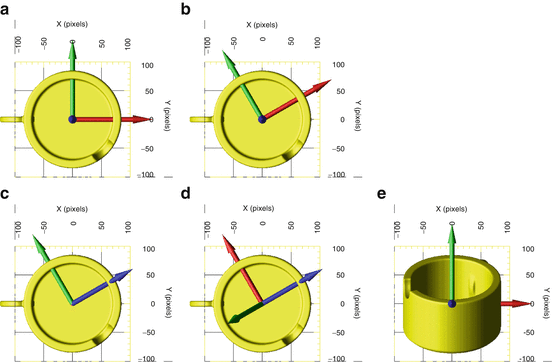

  

  Example of rotation keeping the object fixed and rotating only the coordinate axes. Note that in this approach the system of coordinates formed by the three arrows is not attached to the volume, that is, the volume does not rotate. (a) Original, unrotated system of coordinates. (b) System of coordinates after rotating 30^∘ about Z. (c) System of coordinates after rotating 60^∘ about Y. (d) System of coordinates after rotating 90^∘ about Z. (e) View of the volume after the system of coordinates formed by the three arrows is used to determine the standard display orientation (X pointing right, Y pointing up, and Z point to the observer; compare this figure to Fig. 2.9d). A movie showing the transformation from (a) to (e) is available at URL http://i2pc.cnb.csic.es/rotationsResources/rotateIntrinsicCoordinate.html

• 3. Rotate the volume about the transformed coordinate axes. The traditional way of describing the Euler angles is “First rotate about Z by ϕ. Then, rotate θ about the new Y. Finally, rotate ψ about the new Z.” We have seen that this description corresponds to the second interpretation of the rotation equation. However, if we misunderstand this point and rotate the object by ϕ and then try to rotate by θ about the new Y ​​, we will be led to a rotation that is not the same as the one obtained by the previous procedures. If we still want to rotate the volume about its new transformed axes, we can get the same rotation as before simply by inverting the order of the rotations as shown in the following derivation (the whole procedure can be visually followed in Fig. 2.11). The first rotation is around Z but using the angle ψ (!). So we use the standard rotation matrix $\tilde{R}_{Z3}(\psi )$. This will give us the new object $V _{Z_{1}}(\tilde{\mathbf{r}}) = V (\tilde{R}_{Z3}^{-1}(\psi )\tilde{\mathbf{r}})$ and a new set of coordinate axes (X′, Y ′, Z′) whose expression in the universal coordinate system is given by the rows of the matrix $\tilde{R}_{Z3}(\psi )$. The second rotation should be performed about the new Y, i.e., Y ′. The rotation matrix of θ radians around Y ′ is given by $\tilde{R}_{Y ^{\prime}}(\theta ) =\tilde{ R}_{Z3}(\psi )\tilde{R}_{Y 2}(\theta )\tilde{R}_{Z3}^{-1}(\psi )$. This produces a new volume $V _{Y _{2}}(\tilde{\mathbf{r}}) = V _{Z_{1}}(\tilde{R}_{Y ^{\prime}}^{-1}(\theta )\tilde{\mathbf{r}}) = V (\tilde{R}_{Y 2}^{-1}(\theta )\tilde{R}_{Z3}^{-1}(\psi )\tilde{\mathbf{r}})$ and a new set of axes (X″, Y ″, Z″) whose expression in the universal coordinate system is given by the rows of the matrix $\tilde{R}_{Z3}(\psi )\tilde{R}_{Y 2}(\theta )$. Finally, the third rotation must be performed about the new Z″ but with angle ϕ (!), whose rotation matrix is $\tilde{R}_{Z^{\prime\prime}}(\phi ) =\tilde{ R}_{Y ^{\prime}}(\theta )\tilde{R}_{Z1}(\phi )\tilde{R}_{Y ^{\prime}}^{-1}(\theta ) =\ldots =\tilde{ R}_{Z3}(\psi )\tilde{R}_{Y 2}(\theta )\tilde{R}_{Z1}(\phi )\tilde{R}_{Y 2}^{-1}(\theta )\tilde{R}_{Z3}^{-1}(\psi )$. This last rotation produces the volume $V _{Z_{3}}(\tilde{\mathbf{r}}) = V _{Y _{2}}(\tilde{R}_{Z^{\prime\prime}}^{-1}(\phi )\tilde{\mathbf{r}}) = V (\tilde{R}_{Z1}^{-1}(\phi )\tilde{R}_{Y 2}^{-1}(\theta )\tilde{R}_{Z3}^{-1}(\psi )\tilde{\mathbf{r}}) = V \left ({(\tilde{R}_{Z3}(\psi )\tilde{R}_{Y 2}(\theta )\tilde{R}_{Z1}(\phi ))}^{-1}\tilde{\mathbf{r}}\right )$.

  Fig. 2.11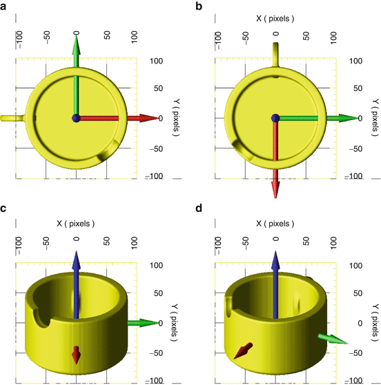

  

  Example of rotation about the transformed axes: (a) Original, unrotated volume. (b) Volume after rotating 90^∘ about Z (blue arrow in (a)). (c) Volume after rotating 60^∘ about the new Y (Y ′, green arrow in (b)). (d) Volume after rotating 30^∘ about the new Z (Z″, blue arrow in (c); compare to Fig. 2.10e). A movie showing the transformation from (a) to (d) is available at http://i2pc.cnb.csic.es/rotationsResources/rotateVolumeIntrinsic.html

2.2.2 Orienting Projections

On many occasions it is useful to have an intuitive idea of the projection orientation given some Euler angles. The formal definition has already been given in Eq. (2.6). In the following, we provide a “manual” rule of how to determine the projection direction and its in-plane rotation given (ϕ, θ, ψ). An easy way to do this is depicted in Fig. 2.12. First, the tilt angle is applied, moving the projection coordinate system and the projection ray (in red) along the “meridian” that passes through X. Then, we move ϕ degrees around the “parallel” in which we previously stopped. Finally, you rotate the projection, in-plane, according to ψ. These movements define the “camera” coordinate system, and the projection will be computed as line integrals in the direction parallel to Z′.

Fig. 2.12

(a) Original projection orientation with $\phi =\theta =\psi = 0$. (b) Apply the tilt angle θ with the projection ray (in red) bound to the projection coordinate system. (c) Apply the rotational angle ϕ. (d) Finally, apply the in-plane rotation

Appendix 3

2.3.1 Mirroring Using Euler Angles

Let us assume that the rotation matrix $\tilde{R}$ can be represented by the ZYZ Euler angles (ϕ, θ, ψ). Now, we are interested in finding some angles (ϕ′, θ′, ψ′) such that

$$\displaystyle{ \tilde{R}(\phi ^{\prime},\theta ^{\prime},\psi ^{\prime}) =\tilde{ M}_{3D}\tilde{R}(\phi,\theta,\psi ). }$$

(2.75)

We first note that $\tilde{M}_{3D} =\tilde{ R}_{X}(\pi ) =\tilde{ R}_{Y }(\pi )\tilde{R}_{Z}(\pi )$, then expanding the definition of each side of the equation, we have

$$\displaystyle{ \begin{array}{ccc} \tilde{R}_{Z}(\psi ^{\prime})\tilde{R}_{Y }(\theta ^{\prime})\tilde{R}_{Z}(\phi ^{\prime})& =&\tilde{R}_{Y }(\pi )\tilde{R}_{Z}(\pi )\tilde{R}_{Z}(\psi )\tilde{R}_{Y }(\theta )\tilde{R}_{Z}(\phi ) \\ & =& \tilde{R}_{Y }(\pi )\tilde{R}_{Z}(\psi +\pi )\tilde{R}_{Y }(\theta )\tilde{R}_{Z}(\phi ) \\ & =& \tilde{R}_{Z}(-(\psi +\pi ))\tilde{R}_{Y }(\theta +\pi )\tilde{R}_{Z}(\phi ),\\ \end{array} }$$

(2.76)

where we have made use of the fact that $\tilde{R}_{Y }(\pi )\tilde{R}_{Z}(\alpha ) =\tilde{ R}_{Z}(-\alpha )\tilde{R}_{Y }(\pi )$. Thus, we see that the angles of the mirrored version of $I_{\tilde{R}}(\tilde{\mathbf{s}})$ are $(\phi,\theta +\pi,-(\psi +\pi ))$. This is a relatively trivial operation, and it provides some intuitive insight on how the two projection directions are related (the azimuthal angle is the same (ϕ), and the tilt angle (θ) is just the opposite in the projection sphere).

2.3.2 Mirroring Using Quaternions

If we perform the same exercise using quaternions, $\tilde{M}_{3D}$ is represented by the quaternion q _{(1, 0, 0), π} . Let us assume that matrix $\tilde{R}$ is represented by some unitary quaternion q _u, α  = (a, b, c, d). The composition of rotations $\tilde{M}_{3D}\tilde{R}$ is represented by the multiplication of quaternions

$$\displaystyle{ \begin{array}{ccl} q_{\mathbf{u}^{\prime},\alpha ^{\prime}} = q_{(1,0,0),\pi }q_{\mathbf{u},\alpha }& =&(-a,d,-c,b) \\ & =&\sin ( \tfrac{\alpha }{2}) + (\cos ( \tfrac{\alpha }{2})\mathbf{e}_{x} +\sin ( \tfrac{\alpha }{2})\mathbf{e}_{x} \times \mathbf{u}),\end{array} }$$

(2.77)

where e _x ^T = (1, 0, 0). Although the operation at the quaternion component level is trivial (some rearrangements and changes of signs), we have totally lost any intuition about how the two projection directions (mirrored and not mirrored) are related.

References

Alsina M, Bayer IP (2004) Quaternion orders, quadratic forms, and Shimura curves. American Mathematical Society, Providence
Baldwin PR, Penczek PA (2007) The transform class in sparx and eman2. J Struct Biol 157(1):250–261
Cantele F, Zampighi L, Radermacher M, Zampighi G, Lanzavecchia S (2007) Local refinement: An attempt to correct for shrinkage and distortion in electron tomography. J Struct Biol 158:59–70
Crowther RA, Henderson R, Smith JM (1996) MRC image processing programs. J Struct Biol 116:9–16
Dalarsson M, Dalarsson N (2005) Tensors, relativity and cosmology. Elsevier Academic Press, San Diego
Frank J, Radermacher M, Penczek P, Zhu J, Li Y, Ladjadj M, Leith A (1996) SPIDER and WEB: Processing and visualization of images in 3D electron microscopy and related fields. J Struct Biol 116:190–199
Grigorieff N (2007) Frealign: High-resolution refinement of single particle structures. J Struct Biol 157:117–125
Harauz G (1990) Representation of rotations by unit quaternions. Ultramicroscopy 33:209–213
van Heel M, Harauz G, Orlova EV, Schmidt R, Schatz M (1996) A new generation of the IMAGIC image processing system. J Struct Biol 116:17–24
Heymann B, Belnap D (2007) Bsoft: Image processing and molecular modeling for electron microscopy. J Struct Biol 157:3–18
Heymann JB, Chagoyen M, Belnap DM (2005) Common conventions for interchange and archiving of three-dimensional electron microscopy information in structural biology. J Struct Biol 151:196–207
Jain AK (1989) Fundamentals of digital image processing. Prentice-Hall, Upper Saddle River
Koks D (2006) Explorations in mathematical physics. Springer, New York
Kremer JR, Mastronarde DN, McIntosh JR (1996) Computer visualization of three-dimensional image data using imod. J Struct Biol 116:71–76
Kuipers JB (1999) Quaternions and rotation sequences. Princeton University Press, Princeton
Ludtke SJ, Baldwin PR, Chiu W (1999) EMAN: Semiautomated software for high-resolution single-particle reconstructions. J Struct Biol 128:82–97
Rossmann MG, Blow DM (1962) The detection of sub-units within the crystallographic asymmetric unit. Acta Crystallogr 15:24–31
Scheres SHW, Valle M, Núñez R, Sorzano COS, Marabini R, Herman GT, Carazo JM (2005) Maximum-likelihood multi-reference refinement for electron microscopy images. J Mol Biol 348:139–149
Shoemake K (1994) Euler angle conversion. In: Graphic gems IV. Academic, San Diego, pp 222–229
Sorzano COS, Marabini R, Velázquez-Muriel J, Bilbao-Castro JR, Scheres SHW, Carazo JM, Pascual-Montano A (2004) XMIPP: A new generation of an open-source image processing package for electron microscopy. J Struct Biol 148:194–204
Sorzano COS, Bilbao-Castro JR, Shkolnisky Y, Alcorlo M, Melero R, Caffarena-Fernández G, Li M, Xu G, Marabini R, Carazo JM (2010) A clustering approach to multireference alignment of single-particle projections in electron microscopy. J Struct Biol 171:197–206
Acknowledgements
The authors would like to acknowledge economical support from the Spanish Ministry of Economy and Competitiveness through Grants AIC-A-2011-0638, BFU2009-09331, BIO2010-16566, ACI2009-1022, ACI2010-1088, CAM(S2010/BMD-2305), and NSF Grant 1114901, as well as postdoctoral Juan de la Cierva Grants with references JCI-2011-10185 and JCI-2010-07594. C.O.S. Sorzano is recipient of a Ramón y Cajal fellowship. This work was funded by Instruct, part of the European Strategy Forum on Research Infrastructures (ESFRI), and supported by national member subscriptions. The research leading to these results has received funding from the European Community’s Seventh Framework Programme (FP7/2007-2013) under BioStruct-X (grant agreement No. 283570).
Author information
Authors and Affiliations
Corresponding author
Editor information
Editors and Affiliations