
Abstract
In Chap. 1 through 8 we discussed both discrete and continuous beam models that can be used to describe the behavior of vibrating systems. We also detailed experimental techniques that we can use to identify these models. In this chapter, we will introduce an approach to combine models or measurements of individual components in order to predict the assembly’s frequency response function (FRF). This method is referred to as receptance coupling (Bishop and Johnson 1960); recall from Sect. 7.1 that a receptance is a type of FRF.
This is a preview of subscription content, log in via an institution.
Buying options
Tax calculation will be finalised at checkout
Purchases are for personal use only
Learn about institutional subscriptionsNotes
- 1.
We will follow this lower case/upper case notation to differentiate between component and assembly coordinates throughout the chapter.
- 2.
We will not consider axial or torsional vibrations in this analysis.
- 3.
Compliance is the inverse of stiffness.
References
Bishop R, Johnson D (1960) The mechanics of vibration. Cambridge University Press, Cambridge
Burns T, Schmitz T (2005) A study of linear joint and tool models in spindle-holder-tool receptance coupling. In: Proceedings of 2005 American Society of Mechanical Engineers International Design Engineering Technical Conferences and Computers and Information in Engineering Conference, DETC2005-85275, Long Beach
Burns T, Schmitz T (2004) Receptance coupling study of tool-length dependent dynamic absorber effect. In: Proceedings of American Society of Mechanical Engineers International Mechanical Engineering Congress and Exposition, IMECE2004-60081, Anaheim
Duncan GS, Tummond M, Schmitz T (2005) An investigation of the dynamic absorber effect in high-speed machining. Int J Mach Tool Manu 45:497–507
Park S, Altintas Y, Movahhedy M (2003) Receptance coupling for end mills. Int J Mach Tool Manu 43:889–896
Schmitz T, Powell K, Won D, Duncan GS, Sawyer WG, Ziegert J (2007) Shrink fit tool holder connection stiffness/damping modeling for frequency response prediction in milling. Int J Mach Tool Manu 47(9):1368–1380
Weaver W Jr, Timoshenko S, Young D (1990) Vibration problems in engineering, 5th edn. Wiley, New York
Acknowledgments
The authors gratefully acknowledge the contributions of Dr. T. Burns, National Institute of Standards and Technology, in developing the Sect. 9.4 damping analysis.
The authors gratefully acknowledge contributions from Dr. T. Burns, National Institute of Standards and Technology, Dr. M. Davies, University of North Carolina at Charlotte, and Dr. G.S. Duncan, Valparaiso University, to the development of the Sect. 9.6 receptance coupling analysis.
Author information
Authors and Affiliations
Corresponding author
Exercises
Exercises
-
1.
Determine the direct frequency response function, \( \frac{{{X_2}}}{{{F_2}}} \), for the two degree of freedom system shown in Fig. P9.1 using receptance coupling. Express your final result as a function of m, c, k, and the excitation frequency, ω. You may assume a harmonic forcing function, \( {F_2}{e^{{i\omega t}}} \), is applied to coordinate X 2.
Fig. P9.1 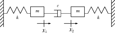
Two degree of freedom assembly
-
2.
Determine the direct frequency-response function, \( \frac{{{X_1}}}{{{F_1}}} \), for the two degree of freedom system shown in Fig. P9.2 using receptance coupling. Express your final result as a function of m, c, k, and the excitation frequency, ω. You may assume a harmonic forcing function, \( {F_1}{e^{{i\omega t}}} \), is applied to coordinate X 1.
Fig. P9.2 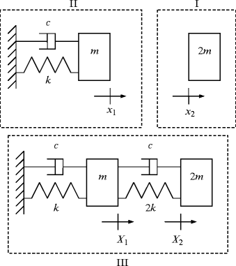
Flexible damped coupling of mass (I) to spring–mass–damper (II) to form the two degree of freedom assembly III
-
3.
Use receptance coupling to rigidly join two free-free beams and find the free-free assembly’s displacement-to-force tip receptance. Both steel cylinders are described by the following parameters: 12.7 mm diameter, 100 mm length, 200 GPa elastic modulus, and 7,800 kg/m3 density. Assume a solid damping factor of 0.0015. Once you have determined the assembly response, verify your result against the displacement-to-force tip receptance for a 12.7 mm diameter, 200 mm long free-free steel cylinder with the same material properties. Select a frequency range that encompasses the first three bending modes and display your results as the magnitude (in m/N) vs. frequency (in Hz) using a semi-logarithmic scale.
-
4.
Plot the displacement-to-force tip receptance for a sintered carbide cylinder with free-free boundary conditions. The beam is described by the following parameters: 19 mm diameter, 150 mm length, 550 GPa elastic modulus, and 15,000 kg/m3 density. Assume a solid damping factor of 0.002. Select a frequency range that encompasses the first three bending modes and display your results as magnitude (m/N) versus frequency (Hz) in a semi-logarithmic format.
-
5.
Determine the fixed-free displacement-to-force tip receptance for a sintered carbide cylinder by coupling the free-free receptances to a rigid wall (with zero receptances). The beam is described by the following parameters: 19 mm diameter, 150 mm length, 550 GPa elastic modulus, and 15,000 kg/m3 density. Assume a solid damping factor of 0.002. Select a frequency range that encompasses the first two bending modes and display your results as magnitude (m/N) versus frequency (Hz) in a semi-logarithmic format. Verify your result by comparing it to the displacement-to-force tip receptance for a fixed-free beam with the same dimensions and material properties.
-
6.
For a rigid coupling between two component coordinates x 1a and x 1b , the compatibility condition is _____________.
-
7.
For a flexible coupling (spring stiffness k) between two component coordinates x 1a and x 1b , the compatibility condition is _____________. An external force is applied to the assembly at coordinate X 1a .
-
8.
For a flexible-damped coupling (spring stiffness k and damping coefficient c) between two component coordinates x 1a and x 1b , the compatibility condition is _____________. An external force is applied to the assembly at coordinate X 1a .
-
9.
What are the units for the rotation-to-couple receptance, p ij , used to describe the transverse vibration of beams?
-
10.
What are the (identical) units for the displacement-to-couple, l ij , and rotation-to-force, n ij , receptances used to describe the transverse vibration of beams?


Rights and permissions
Copyright information
© 2012 Springer Science+Business Media, LLC
About this chapter
Cite this chapter
Schmitz, T.L., Smith, K.S. (2012). Receptance Coupling. In: Mechanical Vibrations. Springer, Boston, MA. https://doi.org/10.1007/978-1-4614-0460-6_9
Download citation
DOI: https://doi.org/10.1007/978-1-4614-0460-6_9
Published:
Publisher Name: Springer, Boston, MA
Print ISBN: 978-1-4614-0459-0
Online ISBN: 978-1-4614-0460-6
eBook Packages: EngineeringEngineering (R0)