Introduction

Abstract

The subject of mechanical vibrations deals with the oscillating response of elastic bodies to disturbances, such as an external force or other perturbation of the system from its equilibrium position. All bodies that possess mass and have finite stiffness are capable of vibrations.

Exercises

• 1. Answer the following questions.

  • (a) All bodies which possess ___________ and ___________ are capable of vibrations.

  • (b) Name the three fundamental categories of vibration.

  • (c) How many degrees of freedom are necessary to fully describe the vibratory motion of an elastic body?

• 2. For the waveform shown below, answer the following questions.

  • (a) Is this motion periodic?

  • (b) If the motion is periodic, what is the period of the motion (in seconds)?

  • (c) If the motion is periodic, what is the frequency of its motion (express your answer in both rad/s and Hz)?

  Fig. P1.2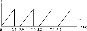

  

  Example waveform

• 3. To explore the Fourier series representation of signals, complete the following.

  • (a) Approximate a square wave by plotting the following function in Matlab ^®. Begin a new m-file by selecting File/New/M-File.

    $\hskip 22pt x = \displaystyle\frac{4}{\pi }\sin \left( {\omega t} \right) + \frac{4}{{3\pi }}\sin \left( {3\omega t} \right) + \frac{4}{{5\pi }}\sin \left( {5\omega t} \right) + \frac{4}{{7\pi }}\sin \left( {7\omega t} \right)$

    Use ω = 2π rad/s and plot your results from t = 0 to 5 s in steps of 0.001 s. You can define your time vector using the following statement:

    

    Also, π can be defined in Matlab ^® using pi. Finally, the argument for sine (or any harmonic function) must be in rad/s in Matlab ^® (not degrees). For example, you can define the displacement using the following statement:

    

    To plot the result, you can use the following statements:

    

  • (b) What is the period (in seconds) of the waveform?

  • (c) What is the frequency in Hz?

  • (d) Replot the function using 50 terms (following the pattern of odd multiples of ω with the $\frac{4}{{n\pi }}$ coefficients where n = 1, 3, 5, …). What is the effect of including additional terms?

• 4. If displacement can be described as $x = 5\cos \left( {\omega t} \right)$ mm, where ω = 6π rad/s, complete the following.

  • (a) Plot the displacement over the time interval from t = 0 to 3 s in steps of 0.02 s. What is the period (in seconds) of the harmonic displacement?

  • (b) Plot the velocity (in mm/s) over the same time interval.

  • (c) Plot the acceleration (in mm/s²) over the same time interval.

  • (d) Calculate the maximum velocity (i.e., calculate the time derivatives and find the maximum values) and acceleration and verify your results using your plots.

• 5. The complex exponential function, $x = {e^{{i\omega t}}}$, can be used to describe harmonic motion (the function can be defined in Matlab ^® using x = exp(1i*omega*t);). Complete the following to explore this function.

  • (a) Plot the real part of the function for ω = π rad/s over a time interval of t = 0 to 10 s using time steps of 0.05 s. Use the command plot(t, real(x)) to complete this task.

  • (b) Plot the imaginary part of the function. Use the command plot(t, imag(x)).

  • (c) Describe your results from parts (a) and (b) in terms of sine and cosine functions.

  • (d) Sketch the Argand diagram for x at t = 0.25 s and show its projections on the real and imaginary axes. What is the numerical value of these projections? How do these results relate to parts (a) and (b)?

• 6. A harmonic motion has an amplitude of 0.2 cm and a period of 15 s.

  • (a) Determine the maximum velocity (m/s) and maximum acceleration (m/s²) of the periodic motion.

  • (b) Assume that the motion expresses the free vibration of an undamped single degree of freedom system and that the motion was initiated with an initial displacement and no initial velocity. Express the motion (in units of meters) in each of the following four forms:

    • $A\cos \left( {{\omega_n}t + {\Phi_c}} \right)$

    • $A\sin \left( {{\omega_n}t + {\Phi_s}} \right)$

    • $B\cos \left( {{\omega_n}t} \right) + C\sin \left( {{\omega_n}t} \right)$

    • $D{e^{{i\left( {{\omega_n}t} \right)}}} + E{e^{{ - i\left( {{\omega_n}t} \right)}}}$.

• 7. Determine the sum of the two vectors ${x_1} = 6{e^{{i\frac{\pi }{6}}}}$ and ${x_2} = - 1{e^{{i\frac{\pi }{3}}}}$.

• 8. If the velocity at a particular point on a body is $v(t) = 250\sin \left( {100t} \right)$, complete the following.

  • (a) Plot the velocity in the complex plane at $t = 0.1$ s.

  • (b) Using the velocity equation, determine the corresponding expression for displacement.

• 9. In bungee jumping, a person leaps from a tall structure while attached to a long elastic cord. Would the resulting oscillation be best described as free, forced, or self-excited vibration?

• 10. The sine function can be represented as $\sin \left( \theta \right) = \theta - \frac{{{\theta^3}}}{{3!}} + \frac{{{\theta^5}}}{{5!}} - \frac{{{\theta^7}}}{{7!}} + \frac{{{\theta^9}}}{{9!}} \cdots$. Plot the percent error between $\sin \left( \theta \right)$ and:

  • $\theta \,\left( {\hbox{rad}} \right)$

  • $\theta - \frac{{{\theta^3}}}{{3!}}\,({\hbox{rad}})$

  • $\theta - \frac{{{\theta^3}}}{{3!}} + \frac{{{\theta^5}}}{{5!}}\,\left( {\hbox{rad}} \right)$

    for a range of $\theta$ values from 0.001 rad to $\frac{\pi }{2}$ rad in steps of 0.001 rad.

    Calculate the percent error using $\left( {\frac{{\theta - \sin \left( \theta \right)}}{{\sin \left( \theta \right)}}} \right)\! \cdot 100$ for the $\theta$ approximation, $\left( {\frac{{\left( {\theta - \frac{{{\theta^3}}}{{3!}}} \right) - \sin \left( \theta \right)}}{{\sin \left( \theta \right)}}} \right) \cdot 100$ for the $\theta - \frac{{{\theta^3}}}{{3!}}$ approximation, and so on. How do these results relate to the small angle approximation?

References

Kreyszig E (1983) Advanced engineering mathematics, 5th edn. Wiley, New York
Schmitz T, Smith KS (2009) Machining dynamics: Frequency response to improved productivity. Springer, New York
Weisstein EW (2010) “Argand diagram” from MathWorld – a Wolfram web resource, http://mathworld.wolfram.com/ArgandDiagram.html
Author information
Authors and Affiliations
Corresponding author