Monitoring

Abstract

Optimizing a server for power, performance, or cost can be achieved with minimal effort. This process begins with monitoring the behavior of a system to understand how it is used and what opportunities exist for improvement. Sensor measurements such as voltage, current, energy, power, and temperature identify individual components that contribute the most to overall server power. Latency, bandwidth, and throughput events illustrate the energy cost of delivering additional performance. Monitoring of power state transitions, clock interrupts, and device interrupts allow users to build a deeper understanding of the distribution of work on a server. This chapter introduces various monitoring capabilities and how they work. It discusses various events and metrics, how these are collected, and what a user can learn from these. Chapter 8 continues with a description of how these events and statistics can be used to guide optimization decisions.

These keywords were added by machine and not by the authors. This process is experimental and the keywords may be updated as the learning algorithm improves.

Optimizing a server for power, performance, or cost can be achieved with minimal effort. This process begins with monitoring the behavior of a system to understand how it is used and what opportunities exist for improvement. Sensor measurements such as voltage, current, energy, power, and temperature identify individual components that contribute the most to overall server power. Latency, bandwidth, and throughput events illustrate the energy cost of delivering additional performance. Monitoring of power state transitions, clock interrupts, and device interrupts allows users to build a deeper understanding of the distribution of work on a server. This chapter introduces various monitoring capabilities and how they work. It discusses various events and metrics, how these are collected, and what a user can learn from these. Chapter 8 continues with a description of how these events and statistics can be used to guide optimization decisions.

System and subcomponent monitoring helps users to improve component selection and future system design. Monitoring aids in software optimization and in identifying issues and opportunities to improve resource usage. Control decisions in management software utilize monitoring, adapting infrastructure to meet changing conditions. For example, management software can monitor processor utilization and memory bandwidth to guide VM migration decisions. Or a CPU can use thermal sensors to identify when to throttle processors down to a lower frequency.

Monitoring features are spread across several subcomponents in the platform. Processors have programmable performance monitoring units in the cores and uncore, baseboards are equipped with power and thermal sensors monitored by management controllers, and operating systems monitor individual application processor, memory, and I/O use. Comparing monitoring data from different subcomponents allows users to build a complete picture of how power and performance affect energy efficiency.

Hardware Monitoring

There are a variety of mechanisms for extracting monitored events or statistics from the CPU. Some of these high-level mechanisms are summarized in Table 7-1. Although each of these mechanisms includes some unique features and capabilities, it is not uncommon for certain events to be tracked through multiple mechanisms.

Table 7-1. Types of CPU Hardware Monitoring

There are a variety of different mechanisms for accessing CPU power statistics. However, the majority of these capabilities require kernel-level permission (administrator in Windows, root in Linux). If you do not have these privileges, these statistics are only available if the system administrator allows common users to access them. These statistics are also commonly not available inside of virtual machines, because the statistics are intended for the system as a whole.

Fixed Counters

A number of fixed counters are available in the system for tracking various statistics. These counters cannot be stopped or cleared (except through CPU cold boot or warm reset). These counters are very useful where the ability to access a common statistic is needed by multiple users at the same time. The downside of fixed counters is that they are restricted from some of the more powerful monitoring techniques.

Core Performance Monitors

Cores on Intel CPUs have used a standard performance monitoring infrastructure for many generations. Dedicated configurable counters (typically four) exist for each hardware thread. A configuration register exists for each counter that allows users to select a specific event to count. In addition to the four configurable counters, three fixed counters exist on the core. All of these are implemented as MSRs and are considered a part of the core performance monitoring architecture. The core performance monitors are covered in detail in the Intel Software Developers Manual (SDM) and therefore will not be covered in detail here. See the following resources for more information:

• www.intel.com/content/dam/www/public/us/en/documents/manuals/64-ia-32-architectures-software-developer-manual-325462.pdf .

• Core performance monitoring events are included as part of the SDM by processor family since these events can change from generation to generation. Core performance monitoring events for each processor are also described in public files (tsv and json) available at the following link: https://download.01.org/perfmon/ .

For monitoring power management, the three fixed counter MSRs (IA32_FIXED_CTR[0,1,2]) in the core can be very powerful. Each of these counters can be configured with the IA32_FIXED_CTR_CTRL MSR to either monitor a specific thread that is executing, or, in the case of processors with SMT, monitor all the threads on the core. The first fixed counter tracks instructions retired, which is a count of every instruction executed by the processor. The second counter tracks unhalted cycles, or cycles when the processor is actively executing instructions. The second counter always counts at the current operating frequency of the processor. The third counter tracks unhalted cycles similar to the second, except it always counts at the base frequency of the processor. Software can use the IA32_FIXED_CTR_CTRL MSR to configure fixed counters to monitor either a specific thread or all threads that share a core. This configuration is done by writing a specific field in the IA32_FIXED_CTR_CTRL MSR called AnyThread. The same MSR interface exposes options to track either user time or kernel time, or both.

Many software tools already exist for monitoring both fixed and programmable core performance monitors (a selection of these are discussed later in the chapter). The simplest way to use a counter is with time-based sampling, using the following steps:

• 1. Clear the counter (to avoid early overflow).

• 2. Configure the desired event in the configuration register and enable the counter.

• 3. Wait some amount of time (while applications execute).

• 4. Read the counter again.

• 5. Repeat steps 1–4.

More advanced techniques are also possible, such as event-based sampling (EBS). In EBS, instead of collecting samples over a fixed amount of time, counters are automatically stopped when one of the counters hits a desired value. At this point, an interrupt is generated that informs monitoring software to collect additional information about system and software state. EBS is not frequently used for monitoring power management and therefore will not be discussed here.

Uncore Performance Monitors

Unlike core performance monitoring, the performance monitoring architecture in the uncore is not standardized across all generations and product lines. A common architecture is used on Xeon E5/E7 products starting in the Sandy Bridge generation. Very few uncore performance monitoring capabilities have been productized on other Intel products, so this chapter will focus on those available in E5/E7.

Uncore performance monitoring introduced in Sandy Bridge is quite similar to the capabilities that exist in the core. Counters are distributed throughout the different blocks in the uncore, providing the ability to collect a large number of statistics simultaneously. Although the bulk of the power-related statistics exist in the counters in the PCU, there are power-relevant events in other blocks too.

Product-specific details of the uncore performance monitoring capabilities and registers are published whenever a product is launched. E5/E7 uncore performance monitoring documentation is included for the latest generation of products at the following links:

• www.intel.com/content/dam/www/public/us/en/documents/design-guides/xeon-e5-2600-uncore-guide.pdf

• www-ssl.intel.com/content/dam/www/public/us/en/documents/manuals/xeon-e5-2600-v2-uncore-manual.pdf

• www.intel.com/content/www/us/en/processors/xeon/xeon-e5-v3-uncore-performance-monitoring.html

Global Freeze/Unfreeze

A challenge with uncore performance monitoring is coordination between the large number of monitoring units spread across various uncore blocks. Simply reading all the counters across those blocks can take tens of microseconds. This latency can both perturb workload execution (particularly if sampling is done over very short time windows) and risk collecting statistics about the monitoring software as opposed to the workload of interest. As a result, the uncore performance monitoring architecture includes a global “freeze” and “unfreeze” capability. This capability attempts to start and stop all counters across various uncore blocks at the same time. Although the synchronization is not perfect, any delay in the freeze of uncore performance monitoring (also known as skid) is typically well below a microsecond.

Edge Detection and Average Time in State

Many monitoring events specify a condition that is counted for every cycle in which that condition is true. For example, if there is an event that monitors the time when a core is in a target C-state, that counter will increment every cycle when the core is in the target C-state. In addition to measuring time in state, it is also useful to be able to monitor the number of transitions in and out of a state. For example, you might want to be able to count the number of times a target C-state was entered. In order to avoid plumbing separate events for both time and transitions, Edge Detect hardware is used, which can transform any event that counts time (or cycles) into an event that counts transitions.

A common monitoring technique is to use one counter to monitor cycles and a separate counter to monitor edges. By using both these events, a user can calculate the average time in a state:

Standard Events and Occupancy Events

Many events simply increment by one in a given cycle. If, for example, you are monitoring the number of reads to DRAM, a standard event would increment by one for each read.

In performance monitoring, when doing queuing and latency analysis, it can be useful to measure the occupancy of different queues. Occupancy events can increment by one or more in each cycle. Occupancy events can also be used with a threshold compare to increment by one whenever a queue is at a configurable occupancy or larger.

For performance monitoring, occupancy events are commonly used in the following ways:

• Average latency in a queue

• Average occupancy of the queue

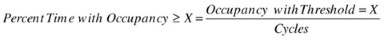
• Time at a given occupancy (or more)¹

Occupancy events can also be applied to power management statistics despite “queues” physically not being a common part of power management. For example, one may want to understand the amount of time when all cores are simultaneously in a core C6 state. By looking at individual core residencies, it is impossible to tell how the different core activity lines up in time. By using an occupancy event for a core C6 state with a threshold set to the number of cores in the system, you can count the amount of time when all cores are simultaneously idle.

Status Snapshots

Snapshots provide an instantaneous view of system characteristics. These are particularly useful for information that does not change very often (like temperature). One drawback of status snapshots is that monitoring software can accidentally collect information about itself. For example, if processor frequency is being measured by monitoring software at a high sampling rate, it may cause frequency to increase higher than it normally would without monitoring software present.

Counter Access and Counter Constraints

Reading or writing from counters and snapshots typically takes a moderate amount of time. It can take tens of clock cycles to access core programmable counters and hundreds of clock cycles to access uncore and other counters. By collecting a large amount of information from throughout, the system can perturb workloads. The amount of statistics collected can have a large impact on the size of sampling that can be performed. Typically, sampling faster than about every 10 ms can lead to significant workload perturbations.

Counters can be implemented in the processor in different ways. Large hardware counters can be quite expensive (area, power) and are not always desirable—particularly in area-constrained blocks or those that are replicated many times. It is also difficult or impossible to provide instantaneous information about certain types of information, for example, in counters for monitoring energy consumption. Statistics about energy are very expensive to monitor accurately through regular synchronous logic. As a result, some fixed counters are updated periodically with this information rather than instantaneously.

Events and Metrics

Monitoring mechanisms described in the preceding section support a wide variety of different measurable events such as core temperature, uncore P-state transitions, or cache lines transferred over a CPU interconnect. Events typically measure a precise low-level occurrence, behavior, or time in state. Events by themselves often do not provide meaningful insight into system or subcomponent behavior. As a result, it is common to use one or more low-level events to calculate a higher-level power or performance metric. For example, a common metric for memory performance is bandwidth. This is calculated based on a number of low-level events such as CAS commands, DDR frequency, and the measurement duration in DDR clock cycles.

Events and metrics include many different types of statistics. Some examples are time, temperature, energy, voltage, frequency, latency, and bandwidth. Specific events and metrics exist across various subcomponents providing insight into runtime characteristics of the system.

Time (RDTSC)

Most software environments provide mechanisms to access information about time in the system. Generally these APIs are sufficient for collecting information about elapsed time when collecting power and performance monitoring statistics.

There are many different ways to measure time in the system. x86 includes an instruction for getting time—the read time stamp counter (RDTSC), which is available both to user space applications and the kernel. Since it is possible for instructions to execute out of order, RDTSCP (a serializing version of RDTSC) is also provided. This version ensures all preceding instructions have completed before reading the time stamp counter. RDTSC is synchronized both across all the threads on a socket, and across threads in a multi-socket system. The RDTSC instruction returns a cycle count that increments at the rate of the base frequency of the processor. Although there is a centralized clock on each CPU, the time stamp counter is also maintained in the core, making it very fast to access. Unlike some performance monitoring counters, RDTSC counts through all power management states. Several other timers exist on the system, but the time stamp counter is preferred because many of them take much longer to access.

Most software tools will provide APIs to measure elapsed time, so making direct use of the RDTSC instruction is generally not necessary. Although many of the statistics and formulas in this chapter that rely on elapsed time will use delta TSC, this can be replaced with whatever time measurement is provided by a given software environment.

Basic Performance

Two basic performance metrics that are key to understanding energy efficiency are CPI and path length. CPI, or cycles per instruction, measures the average number of CPU cycles it takes to retire a single instruction. This is the inverse of the common performance metric IPC, or instructions per cycle. Low CPI occurs when work is computationally simple, where there is a lack of complex operations, and data references frequently hit in core caches. High CPI occurs when work is computationally complex, high-latency operations are frequent, and many data references need to be satisfied by memory. Software with low CPI maximizes the time various subcomponents can spend in low power idle states. It is more energy efficient than high CPI.

Path length measures the average number of instructions it takes to complete a single unit of work. This unit of work is commonly represented by the throughput metric for a workload of interest. For example, a unit of work might be a single HTTP transaction on a web server, a write to a database, a portion of a complex scientific computation, or a single drive read in an I/O testing tool. Beyond the obvious performance advantages, software with low path length also maximizes the time spent in low power idle states since fewer steps are necessary to complete a unit of work.

Performance can be improved either through completing work faster (decreasing CPI), or by completing work using fewer steps (decreasing path length). In the following formula, performance represents the time it takes to complete a unit of work. As a result, performance can generally be expressed by multiplying CPI by path length. The following formulas show how to calculate these basic performance metrics. These can be monitored per-logical processor, per-core, or per-application process, or they can be averaged to give a system level view.

Energy Use

Energy is monitored through both the socket and memory RAPL features (see Chapter 2 for more details). As part of RAPL, free running energy counters track the amount of joules that are consumed by the processor. All energy measured by RAPL is represented in the same format, called energy units. A single energy unit represents a fixed amount of microjoules of energy consumed. Measuring energy in larger granularity energy units allows a high-resolution energy counter to cover a much broader range of values. However, the specific amount of microjoules an energy unit represents can change from processor generation to generation. The RAPL_POWER_UNIT MSR exposes the energy units that are used for RAPL on a given processor. Bits 12:8 show the energy units. As an example, Sandy Bridge presents a value of 0x10, which corresponds to ∼15.3 microjoule increments (1/2^16).

Note

Energy units can change from generation to generation. Haswell, for example, uses different units (∼61 microjoules) than Sandy Bridge and Ivy Bridge (∼15.3 microjoules).

The amount of energy and average power consumed over a time window can be measured with the following two equations:

Table 7-2 lists the different types of energy statistics available on the processor.

Table 7-2. Energy Statistics

Note

Energy counters are only 32 bits today. On Sandy Bridge, for example, it was possible for the counters to roll over after a few minutes. Similar to a car odometer, when the energy counters overflow, they simply wrap around, starting over at zero. Software that makes use of these counters should detect and adjust for this overflow.

Temperature

Modern processors include numerous temperature sensors that are exposed to software. These sensors are generally only available to kernel-level software, because they typically exist in MSR register space. These sensors are sometimes called digital temperature sensors (DTS). Temperatures are usually quite accurate, particularly close to the throttling temperature point. As temperatures get colder, DTS accuracy tends to degrade.

Most server memory also includes temperature sensors on the DIMMs. This is always the case with RDIMMs, and almost always the case with ECC UDIMMs. These sensors are called thermal sensor on-die (TSOD). A single TSOD exists on the memory DIMM (typically in the middle of the DIMM) rather than having individual sensors in each device. Because DRAM devices can be quite long, it is not uncommon for there to be a large thermal gradient down the length of the DIMM. This is particularly the case where DIMMs are oriented in the same direction as the airflow in the platform. As air passes over devices as it moves down the DIMM, it heats up, causing the “last” device to be much warmer than the first. Platform designers take these gradients into account when designing their thermal solutions. Because the TSOD is in the middle of the devices, it is common for some devices to have higher temperatures and some to have lower temperatures.

Rather than exposing the actual temperature in degrees Celsius, temperature counters report the margin to throttle (or the delta between the maximum allowed temperature and the current temperature). The margin to throttle is measured at a core level through the IA32_THERM_STATUS MSR and at a package level through the IA32_PACKAGE_THERM_STATUS MSR. Package temperature reports the highest temperature across all sensors on the package. This includes any additional thermal sensors that may exist outside the cores. Traditionally, cores have been a hot spot on a server die, but this trend is starting to change on low-power server designs where a larger percentage of the package power budget is spent on I/O power. The maximum allowed temperature needed to calculate the actual temperature in degrees Celsius is measured by the TEMPERATURE_TARGET MSR.

The IA32_THERM_STATUS MSR is thread-scoped, meaning an individual thread can only access temperature information about itself. In some systems, multiple threads can share a single temperature sensor and therefore will always get the same result. In addition to reporting temperature, the IA32_THERM_STATUS MSR also reports log and status information about thermal throttling that may have occurred in the system. The IA32_PACKAGE_THERM_STATUS and TEMPERATURE_TARGET MSRs are package-scoped, meaning that all threads on a socket share the same register (and data). Table 7-3 lists the different types of temperature statistics available on the system.

Table 7-3. Temperature Statistics

Frequency and Voltage

Frequency is one of the most important statistics when it comes to power and performance. There are a wide range of mechanisms for monitoring the operating frequency in the system.

Two primary mechanisms are the thread-scoped IA32_PERF_STATUS and IA32_PERF_CTRL MSRs. The IA32_PERF_STATUS MSR holds the current frequency ratio of the thread that reads it. It also has a non-architectural field that provides guidance on the current operating voltage of the core. The voltage field does not exist on older generation server CPUs but is present in many of the current CPUs. The IA32_PERF_CTRL MSR is the same interface introduced in Chapter 6 that allows the operating system to request a frequency ratio for a given thread. Similar to the IA32_PERF_STATUS MSR, the IA32_PERF_CTRL MSR also has a field for requested voltage, however this is no longer used. Voltage is now autonomously controlled by the package, and writes to these bits have no impact on system behavior. Monitoring both of these registers together allows users to understand the relationship between requested frequency and granted frequency.

On E5/E7 processors starting with Haswell, the uncore has its own frequency and voltage (see Chapter 2 for details). These processors include an UNCORE_PERF_STATUS MSR that holds the current operating ratio of the uncore. This register is not architectural and generally is only exposed on systems that have dynamic control of the uncore ratio.

The IA32_APERF and IA32_MPERF MSRs can be used to measure average frequency over a user-defined time window. These free-running counters are sometimes also called ACNT and MCNT. Technically ACNT and MCNT have no architectural definition. Instead, only the ratio of the two is defined. ACNT counts at the frequency at which the thread is running whenever the thread is active. MCNT counts at the base frequency (P1) of the CPU whenever the thread is active. Neither of these MSRs count when the thread is halted in a thread C1 or deeper C-state.

Recent versions of Windows have started clearing both ACNT and MCNT in the kernel, making it unusable by other software tools. Older versions of Linux (before 2.6.29) also had this behavior. Linux no longer clears these MSRs at runtime so that other software tools (such as turbostat, which is included with the kernel) can make use of the MSRs as well.

Similar to ACNT and MCNT, the fixed counters can also be used to monitor the average frequency of either a core or a specific thread when it is active. This methodology automatically filters out time when a core is asleep. The IA32_FIXED_COUNTER1 MSR increments at the rate of the current frequency whenever a thread (or core) is not halted. The IA32_FIXED_COUNTER2 MSR increments at the rate of the base clock of the processor whenever a core (or thread) is not halted. As discussed in “Core Performance Monitors” earlier in this chapter, when the fixed counter AnyThread bits are set to 0, the counters measure average operating frequency of a specific thread while it is active. When the AnyThread bits are set to 1, the fixed counters measure average operating frequency of the core as a whole.

Note

It is common for different threads in the system to report different average frequencies, even on processors that do not support per-core P-states. This is because the average is only taken while a core is active.

To measure average uncore frequency over a user-defined time window, clocks can be counted in the CPU caching agent using a programmable counter (see uncore monitoring links earlier in this chapter for programming information). The caching agent clocks are stopped in Package C6, so this needs to be taken into account when calculating the average frequency. Table 7-4 lists the different frequency and voltage statistics available on the system.

Table 7-4. Frequency Statistics

C-States

Tables 7-5 and 7-6 list the different C-state statistics available on the system.

Table 7-5. Core C-State Hardware Statistics

Table 7-6. Package C-State Hardware Statistics

Memory Power and Performance

Each memory controller channel on Xeon E5/E7 CPUs includes multiple uncore performance monitoring counters and one fixed counter that counts DCLK² cycles. On recent processor generations, the memory controller clock is gated in deep package states, and the performance monitors will stop counting in this state. Table 7-7 lists key memory power and performance statistics available on the system.

Table 7-7. Memory Power and Performance Statistics

Memory bandwidth directly impacts memory power. Required memory bandwidth also can significantly impact purchasing decisions when building a system.

PCIe Power Management

Little visibility exists into PCIe power management from within the SoC.

QPI Power Management and Performance

A wide range of performance monitors are available for QPI. Tables 7-8 and 7-9 list key QPI power and performance statistics available on the system. The performance monitoring counters in the QPI block count at the clock rate of the logic in that block. The QPI link operates at very high frequencies measured in GT/s (giga transfers per second). Sandy Bridge, for example, operated at frequency up to 8 GT/s. In these designs, a single flit (an 80-bit unit of transfer) of data is transmitted in four transfers (or at a rate of 2 GHz in this example). Starting with Sandy Bridge, the clocks used for the QPI performance monitoring logic ran at half this frequency (or 1 GHz in this example), and the logic can process two flits per cycle.

Table 7-8. QPI Power Statistics

Table 7-9. QPI Performance Statistics

Management Controller Monitoring

Management controllers in the system, including the Baseboard Management Controller (BMC) and the Management Engine (ME) in the PCH, provide broader platform-level monitoring functions. The BMC connects to various busses, sensors, and components in the system, allowing it to act as a centralized monitoring resource covering a large number of different system components. The BMC can also pair monitoring functions with threshold values to generate events, such as an indication that a component’s temperature has exceeded a safe level.

Management controller monitoring complements the monitoring functions provided by the CPU and operating system. The BMC and ME provide access to many unique monitoring events that cannot be monitored elsewhere such as fan speed, power supplies, voltages, and general platform health. It also allows for monitoring while a system is booting, powered off, or unresponsive. As discussed in Chapter 5, management controller monitoring functions are accessed through IPMI.

Component Power Sensors

Great insight is gained by understanding individual component power consumption and how individual components add up to overall platform power. In an ideal monitoring solution, platform power (after PSU efficiency losses) would equal the sum of all the individually measured components. However, most servers can only measure CPU and memory power, leaving an incomplete picture.

Note

A common question is “how does power break down in a system?” One engineering technique is to identify the few components that consume the most power and focus optimization efforts on those. The breakdown of power in a system changes significantly from server to server and many of the individual components in a system only represent a small percentage of overall power.

Additional sensors can be added to the baseboard to measure these missing components, reporting either power or current and voltage. During board design, the cost of adding these enhanced sensors necessary to calculate component power is relatively small, for example, adding VRs that expose readings over the SMBus interface or adding current sensors accessible over I2C. These additional sensors allow the Node Manager (NM) firmware to calculate energy for all components in the platform to identify where unaccounted power is coming from. For example, NM can expose individual energy measurements for PCH, LAN, fans, and the BMC. The current generation of Node Manager supports up to 32 additional monitoring devices so component energy can be monitored in fine-grained detail.

Similar to the use of the CPU energy events, NM energy events are coupled with timestamps so users can read the sensors periodically to calculate power over a desired time window.

Synthetic Sensors

In order to expose more information about the platform, Node Manager adds new synthetic sensors for platform characteristics that cannot be easily measured. Node Manager 3.0 added the ability to report volumetric airflow and outlet temperature. Those values are calculated based on the server chassis characterization process and current readings from fans speed sensors, energy consumed by the platform, and inlet air temperature. External management software can create a heat map from information about the physical location of servers in the datacenter and the reported outlet temperatures. This information can be utilized to improve datacenter efficiency, for example, to dynamically manage cooling set points, identify hotspots, or optimize workload placement decisions.

Sensors and Events

Between the BMC and the ME, there are an extensive number of sensors, events, and metrics provided for monitoring. Table 7-10 provides an example of the leading events used to characterize server energy efficiency. Support for various sensors and the specific names of those sensors can vary by platform, so generic or typical names are used in the table. Many different types of sensors such as error indications, hard drive status, or fault and activity LED status are intentionally left out of the table to focus on those sensors most relevant for power.

Table 7-10. Common Monitoring Events Accessible by IPMI

The usefulness of these events is greatly enhanced when several related events are compared together. For example, monitoring the combination of PSU input and PSU output power enables users to calculate both PSU efficiency and power conversion losses.

Note

In calculating PSU efficiency, it is best to use Pout and Pin values averaged over a longer time window. This method takes into account the capacitance of the PSU and results in more representative values.

When BMC monitoring is measured with a workload representative of production use, it enables users to build a deeper understanding of the interactions between various components. Figure 7-1 illustrates various system component temperatures across a range of server load.

Figure 7-1.

Component temperatures across a range of server load

The component temperature in Figure 7-1 can be compared with Figure 7-2, collected at the same time. Comparison of these figures illustrates how fan speed is increased to keep each component within a safe operating temperature. Analyzing related thermal events in conjunction with component-level power allows operators to gain insight into the efficiency of their cooling solution.

Figure 7-2.

Fan speed across a range of server load

Software Monitoring

Chapter 6 discussed the role operating systems play in selecting power states and how operating systems balance power and performance in managing system resources. Different types of applications running on a system can pose a variety of challenges in scheduling, memory management, and I/O. Operating systems provide comprehensive monitoring capabilities that allow users to analyze this behavior. This analysis enables users to gauge how efficiently their system is running, detect poor application behavior, and discover issues with hardware configuration.

Operating systems track many of the same events that are monitored by the CPU. For example, the operating system and CPU can both monitor kernel and user time. In some cases, the operating system is able to provide unique insight into events not understood by the CPU. Operating systems can track time spent in system calls, time spent in interrupt handlers, and time spent submitting and completing I/O. They can also track time spent by individual processes. These enrichments allow the operating system to provide deeper insight into events such as kernel time. In some cases, the operating system is able to add a different perspective to events measured by both the CPU and operating system. For example, the CPU monitors P-state residency in terms of the states that were granted. The operating system is capable of monitoring P-state residency both in terms of the states that were granted and the states that were requested.

When operating system events are used in conjunction with the CPU events, users can build a deeper understanding of the software/hardware interface. For example, the CPU is capable of measuring a specific effect, such as a core being idle 90% of the time and using only C1. The operating system is capable of measuring a specific cause, such as frequent network interrupt handling on the core with high C1 residency.

Another difference between events measured by the CPU and the operating system is accuracy. CPU events are typically clock-cycle accurate, whereas the accuracy of operating system events can vary between products and versions. For example, some events may only be sampled instead of measured, and some events may only be updated during infrequent clock interrupts.

Events used to monitor resource utilization and kernel functions are common across different operating systems. Although the events themselves are similar, there can be some subtle differences in the event names and in precisely what is being measured. For example, one operating system may include kernel time, queue time, and device time in its measure of drive latency, whereas another operating system may only include device time. This section discusses common operating system events in an operating system–independent fashion. Following an outline of these events, several examples of different operating system–specific tools and usages are provided.

Utilization and Processor Time

The operating system is capable of breaking down active and idle time into a very detailed set of information. These events can be used to determine how much time is spent executing application code to identify applications that are running at unexpected times or to identify applications that are running more frequently than expected. For example, these events can detect an intrusive management or security service that may be keeping the system out of a low power idle state.

Processor time events can be analyzed across logical processors, across cores, or across packages to identify utilization asymmetry. This may indicate misconfigured software or legacy software with poor parallel design that is leading to inefficient operation. These events can also be used to assess resource utilization as activity increases or decreases over time. Several of the charts in this chapter illustrate this type of example, demonstrating how an event changes across the full range of server load. Table 7-11 lists several common events describing processor time.

Table 7-11. Common CPU Utilization Events Exposed by Operating Systems

Figure 7-3 illustrates how the various components of processor time change with increasing server load. At the maximum throughput level, only 85% of time is spent executing application code, with the remaining processor time spent performing common kernel functions such as executing system calls or handling interrupts. Optimizations that decrease system time can yield significant improvements in energy efficiency as it provides additional processor time for applications completing work. For example, enabling interrupt coalescing in a network device can reduce the total number of interrupts, thus reducing system time.

Figure 7-3.

CPU time broken down into various categories

Simultaneous Multithreading (SMT)

When discussing processor time, it is important to revisit the relationship between physical processors and logical processors, or hardware threads in Hyper Threading (HT). Since two logical processors share the cache and execution units of a physical processor, it is possible to drive a physical processor to 100% utilization even when each of the logical processors only runs at 50% utilization. It’s also possible for two logical processors at 50% utilization to only drive physical processor utilization slightly above 50%. For datacenter workloads, it’s common to see physical processor utilization up to 50% higher than the reported logical processor utilization. Figure 7-4 illustrates a typical case where actual physical processor utilization is significantly higher than the logical processor utilization.

Figure 7-4.

CPU time compared between logical and physical processor utilization

Operating systems measure utilization for logical processors, which can give a misleading picture of hardware resource utilization as power consumption, and the use of active and idle power management features are much more closely tied to physical processor utilization. Overall utilization is best measured using the hardware mechanisms described earlier in this chapter.

Virtualization

Virtualization provides several additional challenges in monitoring processor time. If utilization is measured from a virtual machine, it is a measure of virtual processor utilization, or utilization of only the resources made available to that VM. For example, in the case of VM oversubscription, it’s possible for VMs to measure an average virtual processor utilization of 10%, whereas the processors themselves are running much higher than that. As a result, it would be inaccurate to conclude that a system is lightly utilized because the average virtual processor utilization is low.

Similar to the insight that can be gained by comparing physical processor utilization to logical processor utilization, additional insight can be gained be examining virtual processor utilization. For system-level analysis, monitoring is best done from the host perspective. The host has the same monitoring visibility as a native operating system as well as the ability to track individual utilization of various guest VMs.

Processor Power State Requests

Chapters 2 and 4 introduced the idea that not all operating system requests for a particular C-state or P-state are necessarily granted by hardware. For example, the operating system might request a high-frequency P-state and end up getting a lower frequency P-state due to a thermal event. Operating systems have the ability to monitor their own internal state requests in addition to what is granted by hardware. Figures 7-5 and 7-6 illustrate the differences between software-requested states and hardware-granted states in C-state residency. In Figure 7-5, ACPI C2 (hardware C6) is requested across the range of server load, but Figure 7-6 shows it is only actually used between 0% and 20% load.

Figure 7-5.

Comparison of software C-state residency (requested) for ACPI C1 and ACPI C2

Figure 7-6.

Comparison of hardware C-state residency (granted) for ACPI C1 and ACPI C2

Note

In Figures 7-5 and 7-6 the sum of ACPI C1 (hardware C1) and ACPI C2 (hardware C6) residency adds up to total idle time. The remaining time not represented in the figure is active time.

Comparing requested residencies to granted residencies can highlight the effectiveness of various hardware and software control policies. These comparisons identify the source of unexpected state residencies, they illustrate the impact of P-state and C-state coordination between threads, and they can help guide server tuning decisions.

One reason for the substantial differences between requested and granted residencies is that software is monitoring requests at the logical processor level, whereas hardware is monitoring at the physical processor level. If half of the logical processors in a system are requesting C6 and the other half of the logical processors are requesting C1, it is possible that every core is in C1. Any time sibling logical processors are requesting different states, the shallower of the two states is granted.

Another reason for the differences between requested and granted residencies is that hardware is utilizing mechanisms to restrict use of deep C-states where it detects significant latency impact or if the energy cost to enter and exit deep C-states will not be recovered by short idle durations. These mechanisms are described in detail in Chapter 2.

Tables 7-12 and 7-13 list several common events exposed by operating systems to monitor C-state and P-state residency and transitions.

Table 7-12. Common C-State Events Exposed by Operating Systems

Table 7-13. Common P-State Events Exposed by Operating Systems

Scheduler, Processes, and Threads

The scheduler’s decisions in determining how compute resources are allocated, shared, and utilized play a key role in energy efficiency. Monitoring this behavior allows users to gain insights into the interaction and impact of running multiple VMs, applications, or processes concurrently. For example, if an operating system migrates processes too aggressively, the additional time it takes to restore execution context or the additional time it takes to reference remote memory can increase power. If the operating system migrates processes too conservatively, it can cause scalability issues and utilization asymmetry. Cases where one subset of logical processors is running at significantly higher utilization than the other logical processors lead to more aggressive use of higher voltage and frequency states, increasing power.

Chapters 2, 3, 4, and 6 introduced a number of decisions hardware and software power management policies need to make in order to strike the right balance between low power and low latency. The scheduler has similar challenges with similar impacts in balancing between high throughput and low latency. Scheduling decisions that minimize latency can improve transaction response times, but it can come at the cost of energy efficiency. If maximum throughput is decreased to improve latency, it results in a greater number of resources (and power) required to meet a peak performance requirement.

Operators that characterize and understand the behavior of the scheduler, processes and threads can uncover opportunities to tune thread affinity and priority to improve energy efficiency. Table 7-14 lists several common events for monitoring the scheduler.

Table 7-14. Common Scheduler, Process, and Thread Events Exposed by Operating Systems

Interrupts

The frequency of interrupts, the distribution of interrupts across logical processors, the division of interrupt processing between top and bottom halves, and the batching of interrupts provide deeper insight into the distribution of work on a server and how the interrupt processing can affect energy efficiency. For example, when clock or device interrupts occur during idle time, they cause logical processors to exit C-states. A high interrupt rate at low throughput is undesirable because low throughput typically coincides with low utilization. When interrupts occur during active time, they cause processes and threads to be suspended until processing of the interrupt is complete.

Splitting the top from the bottom half of interrupt processing enables the kernel to parallelize interrupt processing when a single logical processor is handling interrupts of a specific type. However, the bottom half doesn’t necessarily execute on the same logical processor that handled the interrupt. Interrupts being processed by a very small number of logical processors can be undesirable. This can drive utilization significantly higher on logical processors handling interrupts and cause the top and bottom half of interrupts to be handled by different logical processors. This introduces additional overhead in scheduling and in accessing shared data that is not resident in one of the logical processor’s local caches. The distribution of hard and soft interrupts can increase the overall number of interrupts due to additional IPIs.

Table 7-15 lists events that can be used to identify how interrupt handling is divided across logical processors.

Table 7-15. Common Interrupt Events Exposed by Operating Systems

Memory

It is critical to monitor both memory usage and locality to determine how an application’s use of memory impacts energy efficiency. Sizing memory capacity to meet, but not exceed application requirements is critical for energy efficiency. If there is an excess of free memory capacity in the system, a significant amount of power consumption comes from memory that provides no performance benefit. Similarly, if there is not enough free memory in the system, performance and efficiency can be crippled by swapping.

Monitoring can also help determine the effectiveness of memory in use. Some applications can utilize a virtually unlimited amount of memory, but it may not be beneficial to do so. For example, applications that use memory as a cache for content stored on drives frequently hit a point of diminishing returns. At this point, use of additional memory only yields minor increases in cache hit rates, trading off a very small performance increase for a large increase in power.

Minimizing the amount of memory references that target a remote processor can provide substantial efficiency improvements. In systems with non-uniform memory access (NUMA), or systems with multiple processor sockets, each processor has faster access to local DRAM than it does to remote DRAM or DRAM attached to different sockets. Many applications aren’t properly optimized for NUMA, which results in an equal amount of local and remote memory accesses. It takes more processor time to complete an operation using remote memory than it does using local memory because the increase in memory latency is reflected in CPU stall cycles.

Note

It is surprising to see environments that apply extensive and aggressive efficiency optimization techniques, yet they continue to use applications not optimized for NUMA. Application NUMA optimization remains one of the more common missed opportunities for improving performance and energy efficiency, especially given that the improvements can be realized without any hardware changes.

Table 7-16 lists common events that can be used to identify how effectively memory is being utilized and to understand the locality of memory references.

Table 7-16. Common Memory Events Exposed by Operating Systems

I/O

Issues due to insufficient I/O performance are critical to identify because they result in the use of more servers (and more power) than necessary to meet performance requirements. I/O bottlenecks can prevent applications from being able to fully utilize CPUs and memory, causing components in the system to consume a significant amount of energy while doing little useful work.

Understanding what is sufficient in terms of I/O performance can be a significant challenge. There is a tremendous range in peak performance between different technologies available today. For example, storage subsystems can use different interfaces (3 Gb/s, 6 Gb/s, or 12 Gb/s), different protocols (SATA, SAS, or FC) and different drive types (HDD or SSD). SSDs can have a tremendous impact on system behavior by removing a latency bottleneck that plagues many workloads. In addition to the technologies being used, peak performance is dependent on I/O type, block or packet size, the mix between reads and writes, or the mix between random and sequential I/O. Operating system monitoring features are key to understanding specific workload characteristics and the limitations of an I/O subsystem.

When monitoring I/O it is important to understand the maximum performance of the I/O subsystem when compared to the necessary performance requirements. This applies to both networking and storage. Figure 7-7 compares peak drive I/O operations per second (IOPS) and drive bandwidth to runtime measurements across a range of server load.

Figure 7-7.

Comparing runtime IOPS and bandwidth to theoretical maximums

I/O bottlenecks are frequently introduced during new technology transitions. CPU and memory performance increase at a very different rate than I/O subsystem performance does. Upgrading to the latest platform may result in very different increases in compute performance compared to I/O performance. Another transition that frequently introduces issues with insufficient I/O performance is virtualization. With several VMs sharing an I/O subsystem, increases in traffic, in resource competition, and in diversity of I/O traffic can cause significant decreases in peak I/O performance.

Some I/O bottlenecks can be addressed through tuning, for example, enabling offloading capabilities in an I/O adapter, segmenting or segregating traffic to specific interfaces, enabling interrupt batching, or using virtualization technologies for directed I/O (VT-d). Table 7-15 lists common events that can be used to monitor I/O performance and to compare runtime performance to peak performance capabilities.

Table 7-17. Common I/O Events Exposed by Operating Systems

Tools

This chapter introduced several low-level mechanisms for configuring and accessing monitoring features. For most uses, this complexity can be managed by software tools rather than by an end user. The following section provides a short description of some common software tools and sample usages. This is not intended to be a comprehensive list of all tools and usages. Rather, it introduces the reader to the type of tools available for monitoring and how they can be used. Extensive documentation for these software tools is available online.

Health Checks

Many times, users are interested in getting a high-level picture of what is going on in the system and are less interested in diving into the architectural and micro-architectural details. There are two common tools for Linux (PowerTOP and turbostat) and two for Windows (Perfmon and Powercfg) that provide an excellent first stop for information about the power characteristics of a system.

Turbostat (Linux)

Turbostat is a simple but powerful tool that is built into the Linux kernel tree. It monitors

• Per-thread: Average frequency, activity

• Per-core: Core C-states, temperature

• Per-package: Temperature, package C-states, package power, core power (where supported), DRAM power

Turbostat has several different command-line options that can come in handy for a range of usage models. Simply running it without any parameters will provide one-second snapshots of a range of statistics. Figure 7-8 shows an example of turbostat output.

Figure 7-8.

Turbostat output from a 3.12 kernel

Turbostat is commonly run alongside a workload to get statistics about the system during the measurement. Note that although the statistics provided are heavily influenced by the workload, it is also affected by anything else running on the system.

>> turbostat <program>

The -v option is a great way to collect a wide range of debug information about the system configuration.

>> turbostat -v

Running turbostat at one-second intervals, particularly on large multi-socket systems, can perturb workload behavior (and the results from the tool). Consider increasing the monitoring interval if statistics at one-second intervals are not necessary. This is particularly useful when trying to collect statistics about an idle system.

>> turbostat -i 2

Turbostat can also be used as a simple tool for monitoring various MSRs in the system. The -m and -M options will read the corresponding MSR one time from each thread for each sample. The -M option will dump a 64-bit output, whereas the -m option does a short output. The following command will dump MSR 0x199 at two-second intervals.

>> turbostat -i 2 -M 0x199

The -C and -c options provide a similar capability, but instead of displaying the raw value of the register, these options provide a dump of the delta between the current sample and the previous sample. This can be useful for monitoring the deltas for counters over time. As an example, the following command will dump the delta in APREF (MSR 0xE7) every one-second sample.

>> turbostat -i 1 -M 0xe7

Not all distributions automatically include the turbostat binary, but it is trivial to compile and use once you have the kernel source. The tool is stand-alone, so if you download a recent kernel (from kernel.org), it will include the source. Turbostat requires that your kernel have MSR support.³

// Extract the kernel source after downloading it

>> tar xf linux-3.12.20.tar.xz

// find the sourcecode and cd to the relevant directory

>> cd linux-3.12.20

>> find . -name turbostat.c

>> cd tools/power/x86/turbostat/

// build the tool

>> make

// make sure that the MSR kernel module is active

>> sudo modprobe msr

// run the tool

>> sudo ./ turbostat

PowerTOP (Linux)

PowerTOP is an open-source tool for characterizing power management and diagnosing power management issues. Like turbostat, it is targeted at various usage models (not just servers). It is a useful addition because it provides some additional information above and beyond what turbostat provides. Some notable additions include average time in C-states and frequency histograms. Powertop also provides a large amount of information targeted at consumer usage models (device idle power). The device statistics tend to be less relevant on servers. Figure 7-9 shows sample output of the tool.

Figure 7-9.

Powertop 2.6.1 idle stats

The basic powertop command line provides slow sample intervals by default (many seconds). This can be useful to minimize the application’s overhead, particularly on idle systems, but it also provides much slower results. The time parameter can speed this up (at the expense of increased CPU overhead).

The --html option will dump an HTML file. By default, this will collect a single measurement of the tool. However, more measurements can be collected, generating multiple HTML files. The --html option can collect statistics over the execution of a workload with the --workload parameter. Similar to turbostat, powertop will collect statistics for the entire system and not just the specified workload.

>> powertop --workload=./test.sh --html=test.powertop.html

Powercfg (Windows)

Powercfg is a Windows command-line tool that enables users to tune lower-level operating system power management settings. It allows users to enable and disable features, change power policies, and identify issues that may impact power management. For example, Powercfg can be used to change settings for hard drive power options during inactivity and to query devices to understand the power states they support.

One of the unique applications of Powercfg is its ability to generate an energy report. This option analyzes the system and reports events and configuration details that may impact power management. The Powercfg energy report gives detailed statistics on idle interruption, device activity, failure of devices to support power states, changes to the operating system timer frequency, and supported power states.

The following example command uses Powercfg to list the different power policies supported by the operating system and indicates that the current active policy is balanced. This setting also corresponds to how the operating system is setting IA32_ENERGY_PERF_BIAS during initialization.

C:\Windows\system32>powercfg -list

Existing Power Schemes (* Active)

-----------------------------------

Power Scheme GUID: 381b4222-f694-41f0-9685-ff5bb260df2e  (Balanced) *

Power Scheme GUID: 8c5e7fda-e8bf-4a96-9a85-a6e23a8c635c  (High performance)

Power Scheme GUID: a1841308-3541-4fab-bc81-f71556f20b4a  (Power saver)

The following example command shows how to create the energy report.

C:\Windows\system32>powercfg.exe /energy

Figure 7-10 shows a sample of the energy report results. In this example, the system is seeing poor package C-state residency, and the energy report has identified that several USB devices are connected to the server that do not have USB selective suspend enabled. This activity is preventing the system from maximizing residency in its lowest idle power state.

Figure 7-10.

A portion of the energy report generated by the Windows Powercfg tool

Hardware Monitoring Tools

Programming and reading the various performance counters in the core and uncore of a processor can become fairly complicated. In order to simplify this task, there are a number of stand-alone tools that perform the event programming, data collection, and visualization for the user.

Intel Performance Counter Monitor (PCM)

PCM provides stand-alone tools that handle counter programming and collection for the user. PCM also includes sample routines that demonstrate how to configure and read performance counters with open-source C++ code. These routines translate the raw events into meaningful metrics like memory traffic into GB/s or energy consumed into Joules. PCM is targeted at both power and performance monitoring and characterization and is available as source code with a BSD-like license at www.intel.com/software/pcm .

Intel PCM runs on multiple platforms including Linux, Microsoft Windows, FreeBSD, and Mac OS X. This is possible, because it only requires a driver to program the MSRs. For platforms like Windows, which do not already provide such a driver, the package includes sample code for the driver as well. Binaries are not distributed at the time of publishing, but instructions for compilation are included.

PCM can be used in one of two ways: (1) as a set of stand-alone utilities, or (2) integrated into an application. Figure 7-11 shows an example of a graph generated from data collected by the stand-alone pcm-power utility on a four-socket system.

Figure 7-11.

Socket and DRAM power trace generated from PCM-collected data on four-socket system

The standalone command-line program PCM is similar to turbostat in that it periodically prints the output to the screen for a given time interval. This time interval can be specified as the first parameter. For large servers with tens or hundreds of cores, it is often useful to suppress the metrics for individual cores by using the -nc parameter (for example, > pcm.x 1 –nc). An example from a four-socket system is show in Figure 7-12.

Figure 7-12.

Standalone PCM showing power and performance metrics from a four-socket system

It is also possible to monitor with PCM throughout the duration of a workload by providing the workload executable as a parameter. Since PCM monitors the whole system, the script can actually be a workload driver for a server application that was started beforehand. Please note that in this case, PCM reports the metrics for the entire workload measurement, for example, the total energy consumption.

> pcm.x ./run_workload.sh

For simpler post-processing by spreadsheet program, another convenient feature is the ability to generate comma-separated lists using the -csv option:

> pcm.x 1 -csv 2>&1 | tee pcm.txt

PCM includes a utility targeted exclusively at power management: pcm-power. This utility can measure a number of the statistics made available through the uncore performance monitors on Xeon E5/E7 processors, including these:

• Core C-state residencies

• Causes of frequency throttling (thermal, power, OS requested, electrical/fuse)

• Frequency transition statistics

• Prochot statistics

• Frequency histograms

• DRAM power savings (CKE and self-refresh)

For example, to monitor the number of frequency transitions occurring in the system at one-second intervals (and hide memory statistics), one would execute

> pcm-power.x 1 -p 5 -m -1

Figure 7-13 shows the output of this command. In addition to displaying frequency transition statistics, some power and thermal statistics are also displayed. Additional information is collected using the free-running counters and therefore is displayed regardless of the command line. Note that the DRAM Energy counter was not enabled on the system under test here and therefore reported 0. DRAM RAPL is not a required capability and is not supported on all platforms.

Figure 7-13.

pcm-power screenshot—frequency transitions

Figure 7-14 shows an example where pcm-power is monitoring why the system is unable to achieve the maximum possible frequency (frequency clipping cause) by using the following command line. In this command line, grep is used to filter out some of the extraneous information.

> pcm-power.x 1 -p 3 -m -1 | grep –E "(PCUClocks|limit cycles)"

Figure 7-14.

pcm-power screenshot—frequency clipping cause

The “headroom below TjMax” is shown as 1 or 0, indicating that the system is at the thermal limit. At the same time, the “Thermal freq limit cycles” is hovering at 90%, indicating that the frequency of the system is being limited because of thermal limits a large percentage of the time.

A number of other targeted standalone applications are available as well:

• pcm-numa reports, for each core, the traffic to local and remote memory.

• pcm-memory reports memory traffic per memory channel.

• pcm-pcie reports memory traffic to and from PCIe devices.

• pcm-power can report multiple values depending on the parameter selection.

Both KSysGuard (KDE) and Windows Perfmon provide visualization mechanisms for monitoring individual counters in real time. See the PCM webpage for the latest recipes.

Since PCM is distributed as source code, it can also be integrated directly into an application to facilitate collecting system-wide statistics while an application executes. The initialization is as easy as

PCM * m = PCM::getInstance();

if (m->program() != PCM::Success) return;

The actual measurement is similar to measuring time, where you store the clock before and after the critical code and then take the difference. For the performance counters, there are states available per core, package (socket), and system. There are also predefined functions for all supported metrics:

SystemCounterState before = getSystemCounterState();

// run your code here

SystemCounterState after = getSystemCounterState();

Then, specific statistics can be displayed with, for example, the following:

cout << "Instructions: " << getInstructonsRetired(before, after)

     << "CPU Energy  : " << getConsumedEnergy(before, after)

     << "DRAM Energy : " << getDRAMConsumedEnergy(before, after);

Linux Perf

Newer Linux systems have an integrated profiling and tracing subsystem called perf_events. The perf_events subsystem provides an interface to the CPU’s Performance Monitoring Units (PMUs); it provides an interface to the software tracepoints provided by the Linux kernel, and it takes care of sharing resources between different users. A standard command-line tool called “perf” allows access to the perf_events interface. Other tools and libraries, such as NumaTOP or PAPI, also utilize the perf_events subsystem. There are also GUI frontends available, such as Eclipse perf or sysprof. The perf tool is typically included as a package in the Linux distribution. A wiki with documentation about using perf can be found at https://perf.wiki.kernel.org/index.php/Tutorial .

The perf_events subsystem is integrated into the Linux kernel with the functionality varying depending on kernel version. All perf versions have support for basic PMU profiling with sampling. The perf top utility (shown in Figure 7-15) is an easy way to see details about where the CPU is currently spending its time.

Figure 7-15.

Perf top example

Perf also provides access to software trace points provided by the kernel. For example, perf timechart record records all schedule events and idle periods and can generate a GANTT-style chart with a perf timechart report. This is useful for understanding short stretches (a few seconds) of workload behavior. Timechart first records the system behavior to a perf.data and then generates a SVG file to visualize the trace in a GANTT chart–like representation.

% sudo perf timechart record sleep 1

[ perf record: Woken up 2 times to write data ]

[ perf record: Captured and wrote 1.289 MB perf.data (∼56298 samples) ]

% sudo perf timechart

Written 1.0 seconds of trace to output.svg.

output.svg can then be viewed in a SVG viewer, for example, with Chrome. There are two sets of data provided in the SVG timecharts:

• A view of what is running on each of the logical processors (Figure 7-16)

• A view of the activity of each of the software threads (Figure 7-17)

Figure 7-16.

Timechart part 1: logical processor activity

Figure 7-17.

Timechart part 2: software thread activity

The logical processor information in Figure 7-16 shows both the requested C-states for each of the threads as well as the threads that are active on each of the virtual CPUs (in blue). When cores are asleep, it provides guidance about whether they are waiting for I/O (called the io_schedule routine) or if they are idle and waiting for the CPU (called the schedule routine).

The software thread view in Figure 7-17 shows when each of the different software threads are active (in blue) and when the threads are inactive (in gray). The trace will show the threads starting the first time it sees them execute (and not necessarily when they actually began execution).

In some cases it’s also useful to look at the raw trace events, which can be post-processed with scripts to extract information of interest. The visual timecharts can be challenging to work with on large systems with many threads. The data file generated by the perf timechart record can be viewed with perf script in text format as an alternative to the visual timechart.

% sudo perf script | less

       swapper     0 [000] 176421.261802: power:cpu_idle: state=4 cpu_id=0

       perf      7667 [001] 176421.262026: sched:sched_switch: prev_comm=perf top

       swapper     0 [000] 176421.262692: sched:sched_wakeup: comm=qemu-system

       swapper     0 [000] 176421.262694: power:cpu_idle: state=4294967295 cpu

The first line is the process (swapper means idle), then the pid, CPU number, timestamp, event name, and event parameters. In the first line, CPU 0 goes to sleep with C-state 4. Shortly after, there is a context switch of perf to a thread of top on CPU 1. Then eventually a qemu-system process wakes up CPU 0, which causes an idle exit.

More trace points can be displayed with perf list (as root), recorded with perf record, and displayed with perf script.

A couple of useful tracing features in perf are kprobes and uprobes. These allow you to create new trace points dynamically in the kernel or in user programs. These can be accessed with the perf probe command. The following example sets a probe on the malloc function and measures malloc accesses:

// list functions available

% perf probe -F -x /lib64/libc.so.6  | grep malloc

Malloc

// add a trace point

% sudo perf probe -x /lib64/libc.so.6 malloc

Added new event:

  probe_libc:malloc    (on 0x82520)

// collect a trace

% perf record -e probe_libc:malloc sleep 1

// generate a report from the trace

% perf report

// remove the trace point when done

% perf probe –d probe_libc:malloc

The perf stat command can also be used to access the CPU energy meters (requires kernel 3.14+). The following example command collects package energy use on a single socket system every 100 ms. To get a break down for multiple sockets, --per-socket can be used.

$ sudo perf stat -I100 -e power/energy-pkg/              -a sleep 1

#           time             counts   unit events

     0.100177504              0.25 Joules power/energy-cores/      [100.00%]

     0.100177504              0.86 Joules power/energy-pkg/

...

     0.701274659              0.23 Joules power/energy-cores/

     0.701274659              0.82 Joules power/energy-pkg/

Perf has a simple built-in performance monitoring event list (see perf list). In addition, it is also possible to specify events raw (cpu/event=0x54,umask=0xFF/).

On Xeon E5/E7 processors, it may also be possible to access the uncore events through perf. This can be done with the ucperf.py tool in pmu-tools. This example prints the percentage of time the socket’s frequency is thermally limited every second.

sudo ./ucevent.py  PCU.PCT_CYC_FREQ_THERMAL_LTD

S0-PCU.PCT_CYC_FREQ_THERMAL_LTD

0.00

0.00

0.00

IPMItool

The most frequently used tool to access BMC monitoring capabilities as well as BMC health, inventory, and management functions is IPMItool. This open source command-line tool supports out-of-band access via an authenticated network connection as well as in-band use via a device driver on the server.

The following example demonstrates use of IPMItool by listing the SDR. This command enables users to determine what sensors are available and do a quick check on the status of those sensors. In this example, all but the temperature and thermal sensors have been removed to simplify the example. Specific commands and a full list of available command-line options are available by invoking the tool’s help option, and additional information can be readily found online.

# ipmitool -I lanplus -H xeon-bmc -U root -P pass sdr

BB P1 VR Temp    | no reading        | ns

Front Panel Temp | 22 degrees C      | ok

SSB Temp         | no reading        | ns

BB P2 VR Temp    | no reading        | ns

BB Vtt 2 Temp    | no reading        | ns

BB Vtt 1 Temp    | no reading        | ns

I/O Mod Temp     | no reading        | ns

HSBP 1 Temp      | no reading        | ns

SAS Mod Temp     | 25 degrees C      | ok

Exit Air Temp    | no reading        | ns

LAN NIC Temp     | 35 degrees C      | ok

PS1 Temperature  | 26 degrees C      | ok

PS2 Temperature  | no reading        | ns

P1 Therm Margin  | -59 degrees C     | ok

P2 Therm Margin  | -60 degrees C     | ok

P1 Therm Ctrl %  | 0 unspecified     | ok

P2 Therm Ctrl %  | 0 unspecified     | ok

P1 DTS Therm Mgn | -59 degrees C     | ok

P2 DTS Therm Mgn | -60 degrees C     | ok

P1 VRD Hot       | 0x00              | ok

P2 VRD Hot       | 0x00              | ok

P1 Mem01 VRD Hot | 0x00              | ok

P1 Mem23 VRD Hot | 0x00              | ok

P2 Mem01 VRD Hot | 0x00              | ok

P2 Mem23 VRD Hot | 0x00              | ok

DIMM Thrm Mrgn 1 | no reading        | ns

DIMM Thrm Mrgn 2 | no reading        | ns

DIMM Thrm Mrgn 3 | no reading        | ns

DIMM Thrm Mrgn 4 | no reading        | ns

Mem P1 Thrm Trip | 0x00              | ok

Mem P2 Thrm Trip | 0x00              | ok

Agg Therm Mgn 1  | no reading        | ns

BB +12.0V        | 10.78 Volts       | nc

BB +5.0V         | -1.65 Volts       | cr

BB +3.3V         | 1.91 Volts        | cr

BB +5.0V STBY    | 2.93 Volts        | cr

BB +3.3V AUX     | 1.91 Volts        | cr

BB +1.05Vccp P1  | 1.53 Volts        | cr

BB +1.05Vccp P2  | 1.04 Volts        | ok

BB +1.5 P1MEM AB | 1.48 Volts        | ok

BB +1.5 P1MEM CD | 1.03 Volts        | cr

BB +1.5 P2MEM AB | 1.03 Volts        | cr

BB +1.5 P2MEM CD | 0.78 Volts        | cr

BB +1.8V AUX     | 1.94 Volts        | nc

BB +1.1V STBY    | 1.30 Volts        | cr

BB +3.3V Vbat    | 3.08 Volts        | ok

BB +1.35 P1LV AB | disabled          | ns

BB +1.35 P1LV CD | disabled          | ns

BB +1.35 P2LV AB | disabled          | ns

BB +1.35 P2LV CD | disabled          | ns

BB +3.3 RSR1 PGD | 3.43 Volts        | ok

BB +3.3 RSR2 PGD | 0.65 Volts        | cr

The following example command demonstrates use of IPMItool drill-down into fan-specific sensors. The first example shows how to read the tachometer for connected fans. There are cases where a sensor exists in the SDR, but it is currently not reporting a measurement due to being powered off, disconnected, or unsupported. Disconnected fans have been removed in this example for simplicity.

# ipmitool -I lanplus -H xeon-bmc -U root -P pass sdr type fan

System Fan 1A    | 30h | ok  | 29.1  | 5890 RPM

System Fan 3A    | 34h | ok  | 29.5  | 5890 RPM

System Fan 5A    | 38h | ok  | 29.9  | 5890 RPM

CPU 1 Fan        | 3Ch | ok  | 29.11 | 5820 RPM

CPU 2 Fan        | 3Dh | ok  | 29.12 | 5400 RPM

The sample command in the following example demonstrates use of raw commands to read fan energy sensors. To access lower-level capabilities in the BMC it may be necessary to provide unique one-byte value sequences to indicate a specific command and associated parameters. It is sometimes necessary to use raw commands with IPMItool because not all BMC commands are captured as individual command-line options. Instructions on how to construct raw commands are included in the IPMI specification, and instructions on how to specify associated parameters for the name and location of sensors are captured in documentation provided by the server manufacturer. The names and locations of sensors can vary by platform.

The following command returns energy for one of the fans. The last 8 bytes returned by the command include 4 bytes for running energy in millijoules and 4 bytes for running time in milliseconds. The command is executed twice to illustrate common usage. Periodic reading of these sensors allows users to calculate power. For example, subtracting the first command’s energy from the second command’s energy provides an energy delta. The energy delta between two commands can be divided by the time delta to calculate power.

# ipmitool -I lan -H xeon-bmc -U root -P pass -b 6 -t 0x2c raw 0x2E 0xFB 0x57 01 0x00  0x3 0x0

57 01 00 19 f5 13 01 c7 e3 17 00

# ipmitool -I lan -H xeon-bmc -U root -P pass -b 6 -t 0x2c raw 0x2E 0xFB 0x57 01 0x00  0x3 0x0

57 01 00 f5 54 14 01 fb eb 17 00

Note

IPMItool can also be used to access Node Manager functionality since Node Manager is connected to the BMC using an IPMB link.

More information on component-level power management can be found at www-ssl.intel.com/content/www/us/en/data-center/data-center-management/node-manager-general.html .

Operating System Monitoring Tools

Many times, users are interested in getting a high-level picture of what applications and the operating system are doing and are less interested in diving into the architectural and micro-architectural details. Commonly used tools for Linux (SAR) and Windows (Perfmon and Logman) provide an excellent first stop for information about the power and performance characteristics of software.

SAR

SAR is a Linux tool that monitors processor time, power states, scheduling, memory, I/O, and many other operating system visible events. SAR collects events over a user-defined time interval and outputs many event counts as per-second averages. For several of the monitored events, SAR provides additional detail below a system-level view. For example, processor time can be measured for each individual logical processor, and I/O statistics can be measured for each individual drive or network interface. SAR can be used to gain extensive insight into resource use.

The user-defined time interval and the number of intervals to use in data collection are defined by command-line parameters. For example, the following command specifies -A to measure all events, once per second, over 120 seconds. A full list of available command-line options is available by invoking the tool’s help option, and additional information can be readily found online.

# sar -A 1 120 > sar.dat

The following shows a sample of the output and includes a portion that monitors context switches and interrupts. SAR measures interrupts both at the system level and per IRQ. Users can use SAR output along with /proc/interrupts and /proc/irq/*/smp_affinity to determine what specific devices are generating the interrupts, how frequent they are, and where they are being handled.

08:46:14 PM    proc/s   cswch/s

08:46:24 PM      2.24 104049.64

08:46:14 PM      INTR    intr/s

08:46:24 PM       sum 198321.77

08:46:24 PM        19      1.12

08:46:24 PM        99   7552.09

08:46:24 PM       100   7574.47

08:46:24 PM       101   7297.25

08:46:24 PM       102   7580.26

08:46:24 PM       103   7472.13

08:46:24 PM       104   7808.85

08:46:24 PM       105   7774.36

08:46:24 PM       114   7650.66

08:46:24 PM       115   1660.83

08:46:24 PM       116   1443.44

08:46:24 PM       117   1593.69

08:46:24 PM       118   1750.97

08:46:24 PM       119   1373.35

08:46:24 PM       120   1674.57

08:46:24 PM       123   1417.90

08:46:24 PM       124   1298.17

08:46:24 PM       125   1331.54

08:46:24 PM       126   1375.99

08:46:24 PM       127   1025.64

08:46:24 PM       128   1324.62

08:46:24 PM       129   1425.33

08:46:24 PM       130   1441.81

08:46:24 PM       131      0.71

08:46:24 PM       132      0.51

08:46:24 PM       133      0.51

08:46:24 PM       134      0.51

08:46:24 PM       135      0. 51

Perfmon and Logman

Perfmon is a Windows tool that monitors processor time, power states, scheduling, memory, I/O, and many other events. Perfmon also allows applications to add their own events to the Perfmon infrastructure, allowing users to monitor performance from an application’s perspective alongside the operating system events. Perfmon can be used to develop extensive insight into resource use.

Perfmon events can be visualized in real-time using the GUI (shown in Figure 7-18) or they can be collected for offline analysis using the Windows Logman tool. Logman provides command-line automation of Perfmon as well as other monitoring features such as event traces. It allows users to define different data collectors, or sets of monitoring events, and control when and how the data is collected. Users have the options of creating an always-running monitoring log, initiating different data collection scripts at different times, and writing output to multiple formats.

Figure 7-18.

The Node Manager ACPI Power Metering counters in Performance Monitor showing a power limit being enforced

The Windows typeperf command will list all available Perfmon events on the system. Users can redirect output of this command to a file and edit the file as they see fit to include only the events of interest. The resulting file can then be used as input to Logman to define and create a new data collector. Here is an example of this command:

C:\Windows\System32\typeperf.exe -q > input_file

The following example command creates a new data collector called TEST. Logman includes many command-line options to define collection interval, output format, and output location. A full list of available command-line options is available by invoking the tool’s help option.

C:\Windows\System32\logman create counter TEST

--v -ow -f csv -si 12 -rf 00:01:20 -cf \path \input_file -o \path

The following example command starts the TEST data collector. This will monitor the system for 120 seconds and write to a comma-separated value (CSV) file as defined by the command-line options used to define the data collector.

C:\Windows\System32\logman start TEST

The following output shows a sample of the output including a count of C2 and C1 requests per second issued by the operating system.

12/4/2013 12:53:46 PM        147563.4769         42.47840145

12/4/2013 12:53:58 PM        147825.0577        180.6790098

12/4/2013 12:54:10 PM        149276.3783        120.0697295

12/4/2013 12:54:22 PM        148175.1804         70.16651533

12/4/2013 12:54:34 PM        145440.724          83.24879264

12/4/2013 12:54:46 PM        144713.8251        145.7252465

12/4/2013 12:54:58 PM        146356.6638        112.1651317

12/4/2013 12:55:10 PM        147555.4464        102.7483379

12/4/2013 12:55:22 PM        147615.9768         46.81029614

12/4/2013 12:55:34 PM        148977.9331        106. 331977        

Summary

Numerous capabilities and tools exist for monitoring a system to understand power and performance characteristics. Different types of monitoring capabilities, including hardware monitoring, management controller monitoring, and software monitoring, have unique benefits and usages that aid in understanding system behavior.

Simple metrics can be used to convert raw monitoring data into formats more suitable for analysis, and a number of software tools can aid in visualization. Common monitoring tools, example use, and example output outlined at the end of this chapter provide a quick-start guide for monitoring. Chapter 8 will continue by discussing monitoring techniques that can be used to guide optimization decisions, along with specific examples of tuning.