Multi-Frequency and High Field ESR

Abstract

ESR measurements at high microwave frequency and corresponding high field increase the resolution between species with different g-factors and of g-anisotropies in a single species. Field-independent spectral features due to hyperfine couplings (hfc) and zero-field splittings (zfs) can be separated from g-factor effects by multi-frequency measurements. The zfs for S ≥ 1 species is obtained directly when the microwave frequency is much larger than the zfs. Very large zfs (larger than the microwave energy available) can be indirectly determined by multi-frequency measurements of the effective g-factor. The sign of the zfs (D) can be deduced by high field ESR measurements of the relative intensities of the lines due to zfs. The conditions for obtaining the Heisenberg exchange energy (J) between two species forming a coupled system are considered. Examples of applied studies in the solid state are presented. The influence of forbidden transitions and nuclear spin flip lines frequently complicating the analysis of anisotropic hfc due to ¹H is discussed.

Appendices

Appendix

1.1 A4.1 Hyperfine Splittings by the Direct Field Model for S = ½

The magnetic fields B₊ and B_– acting on a magnetic nucleus is in the direct field model obtained by vector addition of B_N due to the externally applied magnetic field, and ±B_A due to the magnetic moment of the electron.

The magnitude b of B _N corresponds to the nuclear Zeeman energy. The direction is specified by the unit vector l along the applied field:

$${\textbf{B}}_N = - \frac{{\textrm{g}_N \mu _N B}}{{g\mu _B }} \cdot {\textbf{l}} = b \cdot{\textbf{l}}$$

((4.1))

The field B _A can be oriented two ways depending on the value of the electron spin quantum number (m _S = ±½). The field is according to the direct field model [36] given by (4.2) when the electronic g-factor is isotropic:

$$ \pm {\textbf{B}}_A = \pm 1/2 \frac{{\textbf{A}}}{{g\mu _B}}\cdot{\textbf{l}} = \pm \raisebox{3.5pt}{\scriptsize 1}\hbox{/}\raisebox{-2pt}{\scriptsize 2} \cdot \left( {{\textbf{A}}^{\prime}\cdot {\textbf{l}}} \right)$$

((4.2))

The hyperfine coupling is specified in energy and field units by the tensors A and A ^′, respectively. The field B _A is not along the applied field for anisotropic hfc. The strengths of the total fields are therefore given by (4.3):

$$B_ \pm ^2 = \left( { \pm {\textbf{B}}_A + {\textbf{B}}{}_N} \right)^2 = B_A^2 + B_N^2 \pm 2 \cdot {\textbf{B}}_A \cdot {\textbf{B}}_N $$

((4.3))

$$B_ \pm ^2 = \left( {{\textbf{T}}_ \pm \cdot {\textbf{l}}} \right)^2 \quad{\textbf{T}}_ \pm = \pm \raisebox{3.5pt}{\scriptsize 1}\hbox{/}\raisebox{-2pt}{\scriptsize 2} {\textbf{A}}^{\prime} + b{\textbf{E}}$$

((4.4))

The result (4.4) follows from (4.1, 4.2, and 4.3) by algebra that is not reproduced here. One can note, however, that T _± is the tensor commonly employed in the analysis of ENDOR data (Section 3.4.4) with E equal to the unit tensor. The final result (4.4) agrees with that derived more strictly by quantum mechanics methods [26, 36].

The ESR line positions B_o and B_i relative to the centre for the outer and inner doublets of an I = ½ nucleus can be expressed in terms of B _± i.e.:

$$B_0 = \pm \raisebox{3.5pt}{\scriptsize 1}\hbox{/}\raisebox{-2pt}{\scriptsize 2} \left( {B_ + + B_ - } \right)\qquad\qquad B_i = \pm \raisebox{3.5pt}{\scriptsize 1}\hbox{/}\raisebox{-2pt}{\scriptsize 2} \left| {B_ + - B_ - } \right|$$

((4.5))

The intensities of the lines t can be expressed in terms of the angle α between the effective fields for m _S = ±½ by a quantum mechanical treatment, see e.g. [38] for details. The intensities I _i and I _o for the inner and outer doublets of an I = ½ nucleus are given by (4.6):

$$I_i = \cos ^2 \frac{\alpha}{2}\qquad I_o = \sin ^2 \frac{\alpha }{2}$$

((4.6))

The angle α is calculated by quantum mechanics [38] or in the direct field model by applying the cosine theorem (Fig. 4.25) according to equation (4.7):

$$\cos \alpha = \frac{{B_N^2 - B_A^2 }}{{B_ + \cdot B_ - }} = \frac{{b^2 - \left( {\raisebox{3.5pt}{\scriptsize 1}\hbox{/}\raisebox{-2pt}{\scriptsize 2} \cdot {\textbf{A}}^{\prime} \cdot {\textbf{l}}} \right)^2 }}{{B_ + \cdot B_ - }}$$

((4.7))

Fig. 4.25

Effective fields B ₊ (m _S = +½) and B _- (m _S = –½) acting on a nucleus with an anisotropic hfc and a nuclear Zeeman term of comparable magnitude. B _A is due to the hyperfine coupling, B _N to the applied magnetic field

(2·I + 1)² lines are obtained for an arbitrary value of I with intensities and positions given in [38]. In the limits B _N ≪ B _A and B _N ≫ B _A or when the hyperfine coupling is isotropic the normal selection rule Δm _I = 0 applies, yielding 2·I + 1 hyperfine lines of the same intensity. Two equivalent formulations taking account of the combined effects of hyperfine coupling and nuclear Zeeman interaction in case of dominant electron Zeeman energy are commonly employed.

Weil and Anderson formulation [36]: Each electronic level is split in 2·I + 1 sublevels. The splittings in field units for the electronic states m _S = ±½ are given by equation (4.8a):

$$G_ \pm = \sqrt {\left\{ {\sum\limits_{i = 1}^3 {\left[ {\left( { \pm \raisebox{3.5pt}{\scriptsize 1}\hbox{/}\raisebox{-2pt}{\scriptsize 2} \sum\limits_{j = 1}^3 {A_{ij} u_j } } \right) + b_i } \right]} ^2 } \right\}} $$

((4.8a))

The quantities G _± contain contributions from the hyperfine tensor A and from the nuclear Zeeman term $b_i = - B\frac{{g_N \mu _N }}{{g\mu _B }}\ell _i$ where ℓ _x , ℓ _y and ℓ _z are the direction cosines of the applied magnetic field with respect to a suitably chosen coordinate system of a crystal or molecule. In the general case with non-negligible g-anisotropy the effective direction of the field is ${\textbf{u}} = \frac{{{\textbf{g}} \cdot {\textbf{l}}}}{g}$ following the notation of Weil and Anderson [36]. The matrix notation (4.8b) is also employed, e.g. in [26] that also provides the 2nd order corrections reproduced in Chapter 3.

$$G_{m_S }^2 = {\textbf{l}}\left(\frac{{m_S }}{g}{\textit{\textbf{gA}}} + b{\textit{\textbf{E}}}\right)\left(\frac{{m_S }}{g}{\textit{\textbf{Ag}}} + b{\textit{\textbf{E}}}\right){\textbf{l}}$$

((4.8b))

The hyperfine energy for the transition (m _S , m _I ) ↔ (m _S +1, $m_I^{\prime}$) is $\left|{G_{m_S} \cdot m_I - G_{m_S + 1} \cdot m_I^{\prime}}\right|$, where the nuclear quantum numbers m _I and $m_I^{\prime}$ need not be the same. Each nucleus may therefore give (2·I + 1)² rather than the 2·I + 1 hyperfine lines when Δm _I = 0 applies. A spectrum with S = I = ½ has the schematic appearance shown in Fig. 4.26.

Fig. 4.26

S = ½ ESR line pattern for an I = ½ nucleus with an anisotropic hyperfine coupling and a nuclear Zeeman term of comparable magnitude. The inner (i) and outer (o) lines occur at $B_0 \pm \frac{{\left| {G_{1/2}- G_{-1/2}}\right|}}{2}$ and $B_0 \pm \frac{{\left| {G_{1/2}+ G_{-1/2}}\right|}}{2}$ with intensities $I_i = \cos ^2 \frac{\alpha }{2}$ and $I_o = \sin ^2 \frac{\alpha }{2}$, respectively. The angle α is between the effective field directions in Fig. 4.25

Poole and Farach formulation [48]: Equations obtained for the special case with S = I = ½ derived by Poole and Farach [48] are useful when both the inner and outer doublet splittings T _i and T _o are observed. In this case the hyperfine coupling tensor can directly be obtained in single crystal measurements by the Schonland method from the relation:

$${\textbf{l}} \cdot A^2 \cdot {\textbf{l}} = T_0^2 + T_i^2 - \left( {2B_N } \right)^2 $$

((4.9))

It is also of interest that the intensities of the outer and inner doublets can be determined, from measurements of those doublets, using the equations:

$$I_0 = \frac{{T_o^2 - \left( {2g_N \mu _B B} \right)}}{{T_0^2 - T_i^2 }}^2 \qquad I_i = \frac{{\left( {2g_N \mu _B B} \right)^2 - T_i^2 }}{{T_0^2 - T_i^2 }}$$

((4.10))

The hyperfine coupling tensor is not needed to predict the intensities under the condition that the inner and outer doublet splittings are experimentally observed.

Depending on the relative magnitudes of the hyperfine and nuclear Zeeman terms, different cases occur.

(1) Anisotropic g - and A -tensors, negligible b: When the nuclear Zeeman energy is small compared to the hyperfine coupling as is usually the case for transition metal ions, the spectrum is independent of microwave frequency. The hyperfine coupling K depends on the crystal orientation according to the equation (4.11):

$$\left( {g \cdot K} \right)^2 = {\textbf{l}} \cdot {\textbf{g}}A^2 {\textbf{g}} \cdot {\textbf{l}} = \sum\limits_{i,j = 1}^3 {({\textbf{g}}A^2 {\textbf{g}}} )_{ij} \ell _i \ell _j $$

((4.11))

The effective field acting on the nucleus is caused by the hyperfine coupling, so that α ≈180° and the normal selection rule Δm _I = 0 applies. The tensor A ² is accordingly obtained by a modified Schonland procedure described in Chapter 3.

(2) Isotropic g, anisotropic A, non-negligible b: This case occurs particularly for proton hyperfine couplings in organic radicals, but has also been observed for transition metal ions with fluorine ligands [33]. The ¹H and ¹⁹F nuclei have unusually large g _N -factors, and correspondingly large B _N fields in the direct field model. The four line hfc pattern for a single I = ½ nucleus is schematically shown in Fig. 4.26. Formulas that take into account the nuclear Zeeman term on the line positions and intensities were first implemented in the classical works by Lefebvre and Maruani in spectrum simulations of organic radicals with hyperfine structure due to ¹H in amorphous samples. We refer to the literature for the treatment of I = 1 and 3/2 nuclei [38].

(3) Anisotropic A, with principal values ≪ b: Apart from the spin flip lines due to weak dipolar coupling with distant H atoms of the matrix this case is rare at X-band and lower frequencies, but may become of interest for measurements at high microwave frequency bands. The situation is most likely to occur for species with anisotropic hyperfine couplings of moderate size due to nuclei with large nuclear g-factors like ¹H or ¹⁹F. The effective field acting on the nucleus is dominated by the applied field, so that α ≈0 and the normal selection rule Δm _I = 0 applies. The splitting between the lines is $K = {\textbf{l}} \cdot A \cdot {\textbf{l}}$ and $K \cdot g = {\textbf{l}} \cdot \textbf{Ag} \cdot {\textbf{l}}$ for isotropic and anisotropic g-factors, respectively.

(4) Anisotropic A and g, and non-negligible b: The general case with appreciable g- and hyperfine anisotropy and a nuclear Zeeman term that is comparable with the hyperfine coupling is rarely considered in practical applications.

Exercises

• E4.1  

  • (a) Organic radicals typically have g-factors close to the free-electron value g = 2.00232, with only slight anisotropy. In an ESR study of carotenoid and chlorophyll cation radicals in photosystem II at D-band (130 GHz), Lakshmi et al measured g _x = 2.00335, g _y = 2.00251, g _z = 2.00227 [11]. The line-width was 4–5 G. Are the g _x, g _y, and g _z features completely resolved under those conditions? (The spectra are reproduced in Fig. 4.2) Would it be possible to resolve the features corresponding to these g-factors at 385 GHz?

  • (b) Inorganic radicals can have larger g-anisotropies. Can one expect to resolve the g _x = 2.0029, g _y = 2.0225, and g _z = 2.0384 features of the ClSS· radical [F.G. Herring, C.A. McDowell, C. Tait: J. Chem. Phys. 57, 4564 (1972)] at X-band? (The spectrum is reproduced in Chapter 3, Fig. 3.20).

• E4.2 ESR spectra obtained of methyl radicals trapped in a frozen matrix of CO were interpreted by assuming that the radicals rotated rapidly about the three-fold axis of ĊH₃, as shown in the figure. The g-tensor and the hfc-tensor of the three equivalent ¹H atoms are then axially symmetric about this axis. The parameters A _⊥ = 23.4 G, A _|| = 22.3 G, g _⊥ = 2.0027, g _|| = 2.0022, and line-width = 0.43 G were obtained by comparison of experimental and simulated spectra.

  • (a) Examine the shape of the experimental spectrum to explain why it was necessary to consider both g- and hfc-anisotropy in the analysis of the experimental spectrum.

  • (b) Would the observed spectrum look different at Q-band, and if so would the parameters obtained at Q-band be more accurately determined? (Only X-band data were experimentally available).

  • (c) Why can “forbidden” lines due to hfc from ¹H be ignored in the analysis of the experimental spectrum?

    

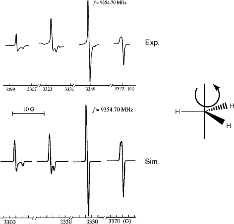
    Experimental and simulated X-band spectra of methyl radicals in a frozen matrix of CO. The figure is reproduced from [Yu.A. Dmitriev, R.A. Zhitnikov: J. Low Temp. Phys. 122, 163 (2001)] with permission from Springer

• E4.3 In the first experimental study of radical pairs by Kurita [40], ESR spectra of the type shown below were observed in single crystal measurements of γ-irradiated dimethylglyoxime at X-band. Suggest an interpretation of the splitting D in the spectrum with H||c^′ and a reason why the splitting appears smaller with H||a^′. What kind of interaction could cause the additional splittings in the spectra?

  

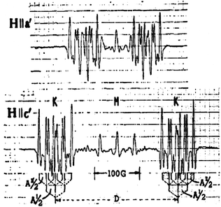
  ESR spectra of irradiated single crystals of dimethylglyoxime at 77 K with the magnetic field directed along the c^′ and a^′ axis. The curves represent 2nd derivatives of the actual absorption spectra. The diagram is reproduced from [40] with permission from the American Institute of Physics

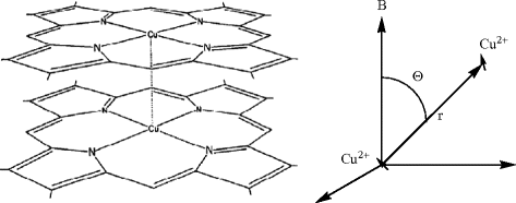
• E4.4 The naturally occurring copper-containing complex, turacin, exhibits ESR spectra of frozen solutions that were interpreted to have a dimer structure containing two Cu²⁺ ions, separated by 3.5 Å. A suggested structure of two turacin molecules forming a sandwich complex obtained from X-band ESR measurements of frozen solutions of samples extracted from touraco feather components is as shown. Magnetic dipolar coupling gives a splitting in two lines separated by $F(T) = \frac{{\mu _0 }}{{4\pi }}\frac{{3\,g\mu _B }}{{2r^3 }}(3\cos ^2 \theta - 1)$. Is first order analysis of the X-band spectra recommendable i.e. is $F < < B_0 = h\nu /g\mu _B \approx 0.33$ T?

  Note: The actual analysis by W.E. Blumberg, J. Peisach: J. Biol. Chem., 240, 870 (1965) was exact, i.e. spectra were calculated by diagonalizing the Hamiltonian matrix, and the zfs and the anisotropic Cu hyperfine structure were adjusted to fit the experimental data.

  

• E4.5 In the paper by Fournel et al. [41] the exchange coupling between a radical and a transition metal complex was found to be positive J = 0.72 cm^–1.

  • (a) How would an energy diagram analogous to that in Fig. 4.21 look like for this antiferromagnetic coupling?

  • (b) Estimate a range of magnitudes of J that would be possible to measure by observing the effect on the spectrum shapes at X-, Q- and W-bands for a coupled system with S ₁ = S ₂ = ½, g ₁ = 1.9, g ₂ = 2.1.

• E4.6 The intensities of the two sets of lines for the radical pair of dimethylglyoxime in the spectra shown in E4.3 are approximately equal at 77 K. At what temperature range would it be possible to determine the sign of D by observing different intensities of the two sets in the ESR spectra at X and W band? Assume that a difference in intensities of ca. 20% is sufficient for the sign assignment.

• E4.7 Suggest a reason why the direct field effect causes complications in ESR but not in ENDOR.

• E4.8 The orientations of the effective fields B _± in Fig. 4.17 determine the quantization axes of the nuclear spin for m _S = ±½.

  • (a) What are the values for the angle α between the axes for the extreme cases $B_N\ll B_A$ and $B_N \gg B_A$ ? Which doublet is observed in each case?

  • (b) What angle applies for isotropic hyperfine couplings? Why do “forbidden” lines not occur in this case?

  Note: Answers can be formally obtained by using formulae in Appendix A4.1. The formulae apply also in the quantum mechanics treatment employed in the first general program for the simulation of ESR spectra of free radicals in amorphous solids [38].

  • (c) Suggest a reason why the spin flip lines tend to become less intense at Q-band than at X-band in the spectra of Fig. 4.19.

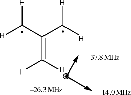
• E4.9 The relative signs of the zfs (D) and the principal values of an anisotropic hfs due to ¹H and ¹⁹F of radical pairs in a single crystal of monofluoroacetamide were determined by analysing the asymmetry of the hyperfine patterns for the m _S = 1 → 0 and m _S = 0 → –1 transitions [39]. The asymmetry is pronounced when the principal hfs couplings are of comparable magnitudes to the nuclear frequencies of ¹H and ¹⁹F. A similar analysis can be applied to triplet state species.

  Would it be more difficult to determine the relative signs of zero-field and hyperfine couplings of triplet state trimethylenemethane by single crystal ESR measurements at W-band than at X-band? The principal values of the six ¹H nuclei are equal and given in the figure.

  

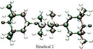
• E4.10 How many hyperfine lines due to ¹⁴N are expected in liquid solution from the “biradical 2” when |J| ≪ |a _N| and |J| ≫ |a _N|, respectively? For details see [K. Komaguchi et al.: Chem. Phys. Lett. 387, 327 (2004)].

  

• E4.11 For most nuclei except ¹H and occasionally ¹⁹F the hyperfine coupling is usually much larger than the nuclear Zeeman energy at X-band.

  • (a) Estimate the magnitude of B _N (Fig. 4.17) for ¹H and ¹⁴N at W-band and discuss possible occurrence of forbidden lines, see Section 3.4.1.2.

  • (b) Estimate the value of B _N for the ¹⁴N nucleus at X-band. Is there any risk of “forbidden” lines due to ¹⁴N hfs for the N₂H₄ ⁺ ion discussed in Chapter 1? Is there such risk for the lines due to ¹H?

References

A.A. Galkin, O.Ya. Grinberg, A.A. Dubinskii, N.N. Kabdin, V.N. Krimov, V.I. Kurochkin, Ya.S. Lebedev, L.G. Oranskii, V.F. Shovalov: Instrum. Exp. Tech. (Eng. Transl.) 20, 284 (1977).
P.C. Riedi, G.M. Smith: In ‘Electron Paramagnetic Resonance’ (Vol. 18) Royal Society of Chemistry Specialist Periodical Reports. Thomas Graham House, Cambridge (2002), pp. 254–303.
A.-L. Barra, A. Gräslund, K.K. Andersson: In ‘Very High Frequency (VHF) ESR/EPR, Biological Magnetic Resonance’ (Vol. 22) ed. by O. Grinberg, L.J. Berliner, Kluwer Academic Publishers, Dordrecht (2004), Chapter 5.
M. Kaupp: In ‘EPR of Free Radicals in Solids, Trends in Methods and Applications’ ed. by A. Lund, M. Shiotani, Kluwer Academic Publishers, Dordrecht (2003), Chapter 7.
D. Goldfarb (guest editor): ‘Modern EPR spectroscopy’, Themed Issue, PCCP 11, 6537 (2009).
W.M. Chen: In ‘EPR of Free Radicals in Solids, Trends in Methods and Applications’ ed. by A. Lund, M. Shiotani, Kluwer Academic Publishers, Dordrecht (2003), Chapter 15.
J.R. Pilbrow: ‘Transition Ion Electron Paramagnetic Resonance’, Clarendon Press, Oxford (1990).
P.W. Atkins, M.C.R. Symons: ‘The Structure of Inorganic Radicals. An Application of ESR to the Study of Molecular Structure’, Elsevier Publishing Company, Amsterdam (1967).
A.Yu. Bresgunov, A.A. Dubinsky, O.G. Poluektov, Ya.S. Lebedev, A.I. Prokof’ev: Mol. Phys. 75, 1123 (1992).
A.L. Barra: Appl. Magn. Reson. 21, 619 (2001).
K.V. Lakshmi, M.J. Reifler, G.W. Brudvig, O.G. Poluektov, A.M. Wagner, M.C. Thurnauer: J. Phys. Chem. B 104, 10445 (2000).
L.E.G. Eriksson, A. Ehrenberg: Acta Chem. Scand. 18, 1437 (1964).
A. Okafuji, A. Schnegg, E. Schleicher, K. Möbius, S. Weber: J. Phys. Chem. B 112, 3568 (2008).
K.C. Christoforidis, S. Un, Y. Deligiannakis: J. Phys. Chem. A 111, 11860 (2007).
D.W. Ovenall, D.H. Whiffen: Mol. Phys. 4, 135 (1961).
A.I. Smirnov: In ‘Electron Spin Resonance Specialist Periodical Reports’ (Vol. 18), ed. by M. Davies, B. Gilbert, N. Atherton, The Royal Society of Chemistry, Cambridge(2002) pp. 109–136.
K.K. Andersson, P.P. Schmidt, B. Katterle, K.R. Strand, A.E. Palmer, S-K Lee, E.I. Solomon, A Gräslund, A-L Barra: J. Biol. Inorg. Chem. 8, 235 (2003).
A.J. Stone: Proc. R. Soc. A. 271, 424 (1963).
F. Neese: EPR Newsl. 18(4), 10, International EPR (ESR) Society (2009).
N.M. Atherton: ‘Principles of Electron Spin Resonance’, Ellis Horwood, New York, NY (1993).
F. Ban, J.W. Gauld, S.D. Wetmore, R.J. Boyd: In ‘EPR of Free Radicals in Solids, Trends in Methods and Applications’ ed. by A. Lund, M. Shiotani, Kluwer Academic Publishers, Dordrecht (2003), Chapter 6.
K.K. Andersson, A.-L. Barra: Spectrochim. Acta A 58, 1101 (2002).
A. Kawamori: In ‘EPR of Free Radicals in Solids, Trends in Methods and Applications’ ed. by A. Lund, M. Shiotani, Kluwer Academic Publishers, Dordrecht (2003), Chapter 13.
H. van der Waals, M.S. de Groot: Mol. Phys. 2, 333 (1959).
M. Iwasaki: J. Magn. Reson. 16, 417 (1974).
J.A. Weil, J.R. Bolton: ‘Electron Paramagnetic Resonance: Elementary Theory and Practical Applications’, 2nd Ed., Wiley, New York, NY (2007).
T. Takui, H. Matsuoka, K Furukawa, S. Nakazawa, K. Sato, D. Shiomi: In ‘EPR of Free Radicals in Solids, Trends in Methods and Applications’ ed. by A. Lund, M. Shiotani, Kluwer Academic Publishers, Dordrecht (2003), Chapter 11.
M. Baumgarten: In ‘EPR of Free Radicals in Solids, Trends in Methods and Applications’ ed. by A. Lund, M. Shiotani, Kluwer Academic Publishers, Dordrecht (2003), Chapter 12.
S. Slappendel, G.A.Veldink, J.F.G. Vliegenthart, R. Aasa, B.G. Malmström: Biochim. Biophys. Acta 624, 30 (1980).
P. Atkins, J. de Paula: ‘Atkins’ Physical Chemistry’, 7th Ed., Oxford University Press, Oxford (2002), p. 632.
C. Chachaty: http://www.esr-spectsim-softw.fr/triplets.htm
C.A. Thuesen, A-L. Barra, J. Glerup: Inorg. Chem. 48, 3198 (2009).
H.M. McConnell, C. Heller, T. Cole, R.W. Fessenden: J. Am. Chem. Soc. 82, 766 (1960).
A. Carrington, A.D. McLachlan: ‘Introduction to Magnetic Resonance with Applications to Chemistry and Chemical Physics’, Harper & Row, New York, NY (1967).
J.A. Weil, J.H. Anderson: J. Chem. Phys. 35, 1410 (1961).
S. Schlick, L. Kevan: J. Magn. Reson. 21, 129 (1976).
R. Lefebvre, J. Maruani: J. Chem. Phys. 42, 1480 (1965).
K. Minakata, M. Iwasaki: Mol. Phys. 23, 1115 (1972).
Y. Kurita: J. Chem. Phys. 41, 3926 (1964).
A. Fournel, S. Gambarelli, B. Guigliarelli, C. More, M. Asso, G. Chouteau, R. Hille, P. Bertrand: J. Chem. Phys. 109, 10905 (1998).
S. Gambarelli, D. Jaouen, A. Rassat, L.C. Brunel, C. Chachaty: J. Phys. Chem. 100, 9605 (1996).
R. Briere, R.M. Dupeyre, H. Lemaire, C. Morat, A. Rassat, P. Rey: Bull. Soc. Chim. France 11, 3290 (1965).
(a) R.B. Clarkson, M D. Timken, D.R. Brown, H.C. Crookham, R.L. Belford: Chem. Phys. Lett. 163, 277 (1989). (b) R.B. Clarkson, D.R. Brown, J.B. Cornelius, H.C. Crookham, W.-J. Shi, R.L. Belford: Pure Appl. Chem. 64, 893 (1992).
Grinberg, L.J. Berliner (eds.): ‘Very High Frequency (VHF) ESR/EPR, Biological Magnetic Resonance’, Vol. 22, Kluwer Academic Publishers, Dordrecht (2004).
Y. Deligiannakis, M. Louloudi, N. Hadjiliadis: Coord. Chem. Rev. 204, 1 (2000).
K. Möbius, A. Savitsky: ‘High-Field EPR Spectroscopy on Proteins and Their Model Systems’, Royal Society of Chemistry, Cambridge (2009).
C.P. Poole, Jr., H.A. Farach: J. Magn. Reson. 4, 312 (1971).
Author information
Authors and Affiliations
Corresponding author