
Abstract
Earth-observation systems (satellites and in situ monitoring) are routinely used to collect information about water quality. Recently, smartphone-based tools and other citizen-science sensors have enabled citizens to also contribute to the collection of scientifically relevant data. This chapter describes a decision support system used to predict optical water-quality indicators in the Wadden Sea, which is an intertidal marine system, where natural processes related to sediment transport and primary production define the basis of its ecological values. As information sources, the system uses satellite data, data collected with a mobile app and physical data for the period 2003–2015. An artificial-intelligence technique, inductive learning, is used to analyze the data and provide predictions in terms of water colour represented via the Forel-Ule scale (a comparative scale for colour).
You have full access to this open access chapter, Download chapter PDF
Introduction
The Wadden Sea is a large-scale, intertidal marine system, where natural processes related to sediment transport and primary production define the basis of its internationally recognized ecological values. Human pressures on the system abound: aquaculture, fishing, tourism and recreation, mining activities, agriculture and industry in the surrounding region. Nutrient inputs from rivers, growing tourism and large-scale fishery activities may create conditions that negatively affect human society, water quality and ecological systems. Satellites and in situ monitoring are routinely used to collect information about water quality (see Fig. 1). Recently, smartphone-based tools and other citizen-science sensors have entered the arena to enable citizens to collect scientifically relevant data (Graham etal. 2011; Ceccaroni and Piera 2017), which can be used by decision support systems. This chapter describes the Citclops Data Explorer: a knowledge-based system designed to predict optical water-quality indicators in the Wadden Sea that may be used for aquaculture, tourism, recreational diving, and water management. As information sources, the system uses MERIS satellite data, data collected with the Citclops—Citizen water monitoring app (Wernand etal. 2012) and physical data: waves, currents, river inputs and weather data for the period 2003–2015 (MERIS data available up to 2011; app data available in 2014–2015).

In situ monitoring platform: yellow markers indicate the Dutch national water quality monitoring network (Rijkswaterstaat); the red pin (NIOZ jetty) indicates the location of the observation platform of the Royal Netherlands Institute of Sea Research (NIOZ). Source: http://kml.deltares.nl/kml/rijkswaterstaat/waterbase/concentration_of_suspended_matter_in_water.kml and Google Earth
Inductive Learning
The inputs to the system were a vector of numerical attribute values, and the target value was a discrete integer. Inductive learning was used to analyse the input data and provide predictions in terms of water colour, using the Forel-Ule (FU) scale, a comparative scale developed in the nineteenth century. The FU scale has an implicit relation to other water-quality properties such as turbidity, transparency, suspended particulate matter and chlorophyll (Wernand 2011). In this way, it is possible to learn a general function or rule from a specific set of input-target value pairs. The system used an artificial-intelligence technique, semi-supervised learning, for capturing the model that establishes the relationship between input and target value pairs. Part of the water colour data was collected by ordinary citizens snapping pictures and being asked to select the most appropriate colour via the Citclops—Citizen water monitoring app. As this is a citizen-science setting, a degree of noise and inaccuracies are expected and dealt with via quality control techniques that involved: the automatic analysis of the photo image, comparison against known satellite measured colour, and flagging of inappropriate measurements via citizen peers.
A system with the ability to predict water quality can be useful in several applications. Apart from direct uses in recreation apps by citizens, it can assist water managers in long-term monitoring, system analysis and decision making on water use. It can provide information to assess the constraints and opportunities for sustainable use of the sea and coast, and also guide risk analysis and response to early warnings. With the information sources mentioned above, an inductive machine learning technique (decision trees) was employed to predict water colour 1 week in the future.
The design of the learning technique took into account three major issues: (1) the output or target value of the model to be learned; (2) the feedback available to system; (3) the representation of the learned model. The target value to be learned was water colour. The type of feedback available determined the nature of the learning problem that the system faced: semi-supervised learning, which involves learning a function from examples of inputs and outputs. The system learned a model represented as a function that maps observations of MERIS satellite data, citizen data and physical data to a discrete output (colour represented as FU). Finally, the representation of the learned information was a decision tree determined by the type of learning algorithms being used. The last major factor in the design of the learning system was the availability of prior knowledge. The system began with no knowledge at all apart from the examples in the data series.
In this study, a machine learning framework is described that uses semi-supervised learning to generate a predictive model that maps marine data coming from heterogeneous sources to a water quality indicator: colour represented by FU. Decision tree induction was used, being one of the most successful forms of learning algorithms, and the model generated is explicit and natural for human data-interpretation. Decision trees take as input a situation described by a set of attributes (from remote sensing, citizens and in situ instruments) and return a decision: the predicted output value for the input, i.e. the prediction of the evolution of FU colour 1 week ahead in time. The input attributes are continuous. The target value is a fixed set of values; therefore the problem can be constructed as a classification learning problem.
Decision trees classify the input vector by performing a sequence of tests. Each internal node in a tree corresponds to a test of the value of one of the attributes in the vector, and the branches from the node are labelled with the possible values of the test. Each leaf node in a tree specifies the value to be returned.
The aim here is to learn a model for the target label FU-Colour.
Data Description
The following list describes the data available to the system:
-
1.
MERIS satellite data: FU, chlorophyll-a (2002–2011)—time resolution: one data point per day (missing data on cloudy days)
-
2.
FU data collected with the Citclops—Citizen water monitoring app (2013–2015)
-
3.
Water quality data: total suspended matter (TSM), FU, chlorophyll-a collected by means of a spectroradiometer mounted on the NIOZ observation platform (2013–2015) (see Figs. 2 and 3)—time resolution: every 2 min during daylight (some missing periods)
Fig. 2 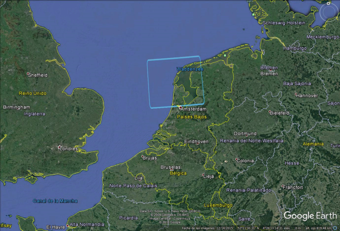
The study area for the 2013–2015 study period is the Wadden Sea, located within the rectangle at the center of the figure. Source: Google Earth
Fig. 3 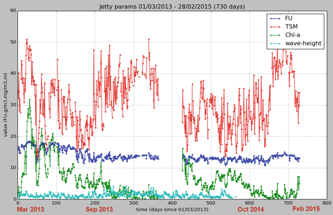
NIOZ jetty Wadden Sea: RS calculated water quality data (TSM, FU, chlorophyll-a) and wave height (daily means)
-
4.
Wave data (2003–2013) (wave height and period)—average time resolution: one data point per hour
-
5.
Water-current data (2003–2013)
-
6.
River inputs, salinity, water temperature (2003–2013)—average time resolution: one data point per day
-
7.
Weather data: insolation, as an extra driver for algal growth; wind speed magnitude, which correlates strongly with wave height; wind direction; and air temperatures (2003–2013)
-
8.
SPM, chlorophyll-a, DOC, K d collected in situ (2003–2013)—average time resolution: two data points per month


Methods
The following Earth observations have been finally used as part of the input: FU colour index, TSM, chlorophyll-a and wave height. A model of the target variable “FU colour” at future points (2 days, 4 days, 7 days) has been learned (see Fig. 4). To do this, the initial problem was converted to a three-class classification problem (see Fig. 5): FU colour decreases, is stable or increases.

Machine-learning pipeline

Conversion to a three-class classification problem
The model’s prediction of FU has been evaluated using tenfold cross-validation. It has then been integrated into the Citclops Data Explorer—Marine Data Analyser (http://citclops-data-explorer.herokuapp.com/marine-data-analyser).
Results and Discussion
Note that every variable used has a small set of possible values or is continuous; the value of FU colour index, for example, is not an integer, rather it is one of the 21 discrete values from 1 to 21. The task of finding a tree that is consistent with the input examples and is as small as possible, no matter how size is measured, is an intractable problem: time grows exponentially with the amount of data and there is no way to efficiently search through the possible trees. With some simple heuristics, however, the authors found a good approximate solution: a small (but not the smallest) consistent tree, defining the sequence of tests and the specification of each test in an acceptable time.
The forecasting system is composed of different decision trees (implemented in Python), which predict if the FU colour decreases, is stable or increases over a week (2 days, 4 days and 7 days in advance). The performance of these decision trees is compared to the one of a support vector machine algorithm and of blind predictors. Samples of the results of the algorithms used are presented in Figs. 6, 7 and 8.

Example of results using a specific feature-configuration and a support vector machine algorithm

Example of results using a specific feature-configuration and random-forest decision trees

Example of results using a specific feature-configuration and decision trees with a maximum depth of 10
Each figure represents the learning protocol and experiment that was performed. The rows of the grid on the top left of the figure are the type of attributes (wave height, TSM, Chl-a, FU), and the columns are consecutive individual days on which the attributes have been measured. The coloured (non-blue) squares mark the feature configuration of the training examples. The column with the squares coloured in orange represent the reference time point (t = 0/present time point) and are part of the input vector. The red squares are attributes that are also included in the input vector but from days before the reference time point. The green square is the attribute that the model will learn to predict which will always be at a future time point in relation with the orange column. In the top right is the learning technique and some key configuration parameters. As an example, in Fig. 6, the target-value attribute is FU at 2 days into the future, and the input vector includes the following attributes: wave height, TSM, Chl-a, FU at the current time point, and wave height at 1 day in the past.
The algorithm used adopts a greedy divide-and-conquer strategy: always test the most important attribute first. This test divides the problem up into smaller sub-problems that can then be solved recursively. By “most important attribute”, the authors mean the one that makes the most difference to the classification of an example. That way, the authors hope to get to the correct classification with a small number of tests, meaning that all paths in the tree will be short and the tree as a whole will be shallow.
In general, after the first attribute-test splits up the examples, each outcome is a new decision-tree learning problem in itself, with fewer examples and one less attribute. There are four cases to consider for this recursive problem:
-
1.
If the remaining examples are all decrease (or stable or increase), then the algorithm provides an answer.
-
2.
If there are some mixed decrease, stable or increase examples, then choose the best attribute to split them.
-
3.
If there are no examples left, it means that no example has been observed for this combination of attribute values, and the algorithm returns a default value calculated from the plurality classification of all the examples that were used in constructing the node’s parent.
-
4.
If there are no attributes left, but both positive and negative examples, it means that these examples have exactly the same description, but different classifications. This can happen because there is an error or noise in the data; because the domain is nondeterministic; or because an attribute that would distinguish the examples has not been observed or taken into account. The algorithm returns in this case the plurality classification of the remaining examples.
The accuracy of the learning protocol is compared in each case to a blind predictor as a benchmark test. The blind predictor always classifies to the most common class in the examples of the training set. In the case of Fig. 8, the most common class is an increase in FU, that occurs 35% of the time. Thus a classifier predicting always an increase would be 35% of time accurate. The accuracy by the decision-tree algorithm is 45% thus suggesting that indeed the model has utilised patterns in the current attributes and past attributes to predict the future value (7 days ahead in time).
Conclusions
In this study, an artificial-intelligence technique, inductive learning, has been used to analyze data from Earth-observation systems, citizens, marine scientists and coastal planners and to provide predictions in terms of water colour, using the Forel-Ule scale, a comparative scale for colour. Specifically, decision trees have been used for learning. Note that the set of data examples is crucial for constructing the trees, therefore the quality of the trees as a classification tool depends on the quality of the original data. Each tree consists of just tests on attributes in the interior nodes, values of attributes on the branches, and output values on the leaf nodes.
These trees are also bound to make some mistakes for cases where they have seen no examples. For example, they have never seen cases of extreme FU values. In future work, with more training examples, the learning program could correct these mistakes.
The authors could identify the following potential applications for these trees:
-
to provide sea farmers with bulletins about algal blooms, which change the water colour;
-
to maximize citizens’ experience in activities in which water quality has a role; and
-
to provide citizens with powerful, user-friendly tools for environmental-data interpretation.
References
Ceccaroni L, Piera J (2017) Analyzing the role of citizen science in modern research. IGI Global, Hershey, PA. https://doi.org/10.4018/978-1-5225-0962-2
Graham EA, Henderson S, Schloss A (2011) Using mobile phones to engage citizen scientists in research. EOS Trans Am Geophys Union 92(38):313–315
Wernand MR (2011) Poseidon’s paintbox: historical archives of ocean colour in global-change perspective. Ph.D. thesis, Utrecht University, p 240. ISSN 978-90-6464-509-9
Wernand MR, Ceccaroni L, Piera J, Zielinski O (2012) Crowdsourcing technologies for the monitoring of the colour, transparency and fluorescence of the sea. In: Proceedings of ocean optics XXI, Glasgow, Scotland, pp 8–12
Author information
Authors and Affiliations
Corresponding author
Editor information
Editors and Affiliations
Rights and permissions
<SimplePara><Emphasis Type="Bold">Open Access</Emphasis> This chapter is licensed under the terms of the Creative Commons Attribution 4.0 International License (http://creativecommons.org/licenses/by/4.0/), which permits use, sharing, adaptation, distribution and reproduction in any medium or format, as long as you give appropriate credit to the original author(s) and the source, provide a link to the Creative Commons license and indicate if changes were made.</SimplePara> <SimplePara>The images or other third party material in this chapter are included in the chapter's Creative Commons license, unless indicated otherwise in a credit line to the material. If material is not included in the chapter's Creative Commons license and your intended use is not permitted by statutory regulation or exceeds the permitted use, you will need to obtain permission directly from the copyright holder.</SimplePara>
Copyright information
© 2018 The Author(s)
About this chapter

Cite this chapter
Ceccaroni, L., Velickovski, F., Blaas, M., Wernand, M.R., Blauw, A., Subirats, L. (2018). Artificial Intelligence and Earth Observation to Explore Water Quality in the Wadden Sea. In: Mathieu, PP., Aubrecht, C. (eds) Earth Observation Open Science and Innovation. ISSI Scientific Report Series, vol 15. Springer, Cham. https://doi.org/10.1007/978-3-319-65633-5_18
Download citation
DOI: https://doi.org/10.1007/978-3-319-65633-5_18
Published:
Publisher Name: Springer, Cham
Print ISBN: 978-3-319-65632-8
Online ISBN: 978-3-319-65633-5
eBook Packages: Physics and AstronomyPhysics and Astronomy (R0)