Model-Free Reinforcement Learning for Branching Markov Decision Processes

Abstract

We study reinforcement learning for the optimal control of Branching Markov Decision Processes (BMDPs), a natural extension of (multitype) Branching Markov Chains (BMCs). The state of a (discrete-time) BMCs is a collection of entities of various types that, while spawning other entities, generate a payoff. In comparison with BMCs, where the evolution of a each entity of the same type follows the same probabilistic pattern, BMDPs allow an external controller to pick from a range of options. This permits us to study the best/worst behaviour of the system. We generalise model-free reinforcement learning techniques to compute an optimal control strategy of an unknown BMDP in the limit. We present results of an implementation that demonstrate the practicality of the approach.

This work was supported by the Engineering and Physical Sciences Research Council through grant EP/P020909/1 and by the National Science Foundation through grant 2009022. This project has received funding from the European Union’s Horizon 2020 research and innovation programme under grant agreement No 101032464 (SyGaST) and 864075 (CAESAR).

1 Introduction

Branching Markov Chains (BMCs), also known as Branching Processes, are natural models of population dynamics and parallel processes. The state of a BMC consists of entities of various types, and many entities of the same type may coexist. Each entity can branch in a single step into a (possibly empty) set of entities of various types while disappearing itself. This assumption is natural, for instance, for annual plants that reproduce only at a specific time of the year, or for bacteria, which either split or die. An entity may spawn a copy of itself, thereby simulating the continuation of its existence.

The offspring of an entity is chosen at random among options according to a distribution that depends on the type of the entity. The type captures significant differences between entities. For example, stem cells are very different from regular cells; parallel processes may be interruptible or have different privileges. The type may reflect characteristics of the entities such as their age or size.

Although entities coexist, the BMC model assumes that there is no interaction between them. Thus, how an entity reproduces and for how long it lives is the same as if it were the only entity in the system. This assumption greatly improves the computational complexity of the analysis of such models and is appropriate when the population exists in an environment that has virtually unlimited resources to sustain its growth. This is a common situation that holds when a species has just been introduced into an environment, in an early stage of an epidemic outbreak, or when running jobs in cloud computing.

BMCs have a wide range of applications in modelling various physical phenomena, such as nuclear chain reactions, red blood cell formation, population genetics, population migration, epidemic outbreaks, and molecular biology. Many examples of BMC models used in biological systems are discussed in [12].

Branching Markov Decision Processes (BMDPs) extend BMCs by allowing a controller to choose the branching dynamics for each entity. This choice is modelled as nondeterministic, instead of random. This extension is analogous to how Markov Decision Processes (MDPs) generalise Markov chains (MCs) [24]. Allowing an external controller to select a mode of branching allows us to study the best/worst behaviour of the examined model.

As a motivating example, let us discuss a simple model of cloud computing. A computation may be divided into tasks in order to finish it faster, as each server may have different computational power. Since the computation of each task depends on the previous one, the total running time is the sum of the running times of each spawned task as well as the time needed to split and merge the result of each computation into the final solution. As we shall see, the execution of each task is not guaranteed to be successful and is subject to random delays. Specifically, let us consider the following model with two different types (T and S), and two actions ($a_1$ and $a_2$). This BMDP consists of the main task, T, that may be split (action $a_1$) into three smaller tasks, for simplicity assumed to be of the same type S, and this split and merger of the intermediate results takes 1 hour (1h). Alternatively (action $a_2$), we can execute the whole task T on the main server, but it will be slow (8 h). Task S can (action $a_1$) be run on a reliable server in 1.6 h or (action $a_2$) an unreliable one that finishes after 1 h (irrespective of whether or not the computation is completed successfully), but with a 40% chance we need to rerun this task due to the server crashing. We can represent this model formally as:

We would like to know the infimum of the expected running time (i.e. the expected running time when optimal decisions are made) of task T. In this case the optimal control is to pick action $a_1$ first and then actions $a_1$ for all tasks S with a total running time of 5.8 h. The expected running time when picking actions $a_2$ for S instead would be $1 + 3 \cdot 1/0.6 = 6$ [hours].

Let us now assume that the execution of tasks S for action $a_1$ may be interrupted with probability 30% by a task of higher priority (type H). Moreover, these H tasks may be further interrupted by tasks with even higher priority (to simplify matters, again modelled by type H). The computation time of T is prolonged by 0.1 h for each H spawned. Our model then becomes:

As we shall see, the expected total running time of H can be calculated by solving the equation $x = 0.3 (x+x) + 0.1$, which gives $x = 0.25$ [hour]. So the expected running time of S using action $a_1$ increases by $0.3 \cdot 0.25 = 0.075$ [hour]. This is enough for the optimal strategy of running S to become $a_2$. Note that if the probability of H being interrupted is at least 50% then the expected running time of H becomes $\infty$.

When dealing with a real-life process, it is hard to come up with a (probabilistic and controlled) model that approximates it well. This requires experts to analyse all possible scenarios and estimate the probability of outcomes in response to actions based on either complex calculations or the statistical analysis of sufficient observational data. For instance, it is hard to estimate the probability of an interrupt H occurring in the model above without knowing which server will run the task, its usual workload and statistics regarding the priorities of the tasks it executes. Even if we do this estimation well, unexpected or rare events may happen that would require us to recalibrate the model as we observe the system under our control.

Instead of building such a model explicitly first and fixing the probabilities of possible transitions in the system based on our knowledge of the system or its statistics, we advocate the use of reinforcement learning (RL) techniques [27] that were successfully applied to finding optimal control for finite-state Markov Decision Processes (MDPs). Q-learning [30] is a well-studied model-free RL approach to compute an optimal control strategy without knowing about the model apart from its initial state and the set of actions available in each of its states. It also has the advantage that the learning process converges to the optimal control while exploiting along the way what it already knows. While the formulation of the Q-learning algorithm for BMDPs is straightforward, the proof that it works is not. This is because, unlike the MDPs with discounted rewards for which the original Q-learning algorithm was defined, our model does not have an explicit contraction in each step, nor does boundedness of the optimal values or one-step updates hold. Similarly, one cannot generalise the result from [11] that estimates the time needed for the Q-learning algorithm to converge within $\epsilon$ of the optimal values with high probability for finite-state MDPs.

1.1 Related Work

The simplest model of BMCs are Galton-Watson processes [31], discrete-time models where all entities are of the same type. They date as far back as 1845 [14] and were used to explain why some aristocratic family surnames became extinct. The generalisation of this model to multiple types of entities was first studied in 1940s by Kolmogorov and Sevast’yanov [17]. For an overview of the results known for BMCs, see e.g. [13] and [12]. The precise computational complexity of decision problems about the probabilities of extinction of an arbitrary BMC was first established in [9]. The problem of checking if a given BMC terminates almost surely was shown in [5] to be strongly polynomial. The probability of acceptance of a run of a BMC by a deterministic parity tree automaton was studied in [4] and shown to be computable in PSPACE and in polynomial time for probabilities 0 or 1. In [16] a generalisation of the BMCs was considered that allowed for limited synchronisation of different tasks.

BMDPs, a natural generalisation of BMCs to a controlled setting, have been studied in the OR literature e.g., [23, 26]. Hierarchical MDPs (HMDPs) [10] are a special case of BMDPs where there are no cycles in the offspring graph (equivalently, no cyclic dependency between types). BMDPs and HMDPs have found applications in manpower planning [29], controlled queuing networks [2, 15], management of livestock [20], and epidemic control [1, 25], among others. The focus of these works was on optimising the expected average, or the discounted reward over a run of the process, or optimising the population growth rate. In [10] the decision problem whether the optimal probability of termination exceeds a threshold was studied: it was shown to be solvable in PSPACE and at least as hard as the square-root sum problem, but one can determine if the optimal probability is 0 or 1 in polynomial time. In [7], it was shown that the approximation of the optimal probability of extinction for BMDPs can be done in polynomial time. The computational complexity of computing the optimal expected total cost before extinction for BMDPs follows from [8] and was shown there to be computable in polynomial time via a linear program formulation. The problem of maximising the probability of reaching a state with an entity of a given type for BMDPs was studied in [6]. In [28] an extension of BMDPs with real-valued clocks and timing constraints on productions was studied.

1.2 Summary of the Results

We show that an adaptation of the Q-learning algorithm converges almost surely to the optimal values for BMDPs under mild conditions: all costs are positive and each Q-value is selected for update independently at random. We have implemented the proposed algorithm in the tool Mungojerrie [21] and tested its performance on small examples to demonstrate its efficiency in practice. To the best of our knowledge, this is the first time model-free RL has been used for the analysis of BMDPs.

2 Problem Definitions

2.1 Preliminaries

We denote by $\mathbb N$ the set of non-negative integers, by $\mathbb R$ the set of reals, by ${\mathbb R}_{+}$ the set of positive reals, and by ${\mathbb R}_{\ge 0}$ the set of non-negative reals. We let ${\widetilde{\mathbb R}}_{+}= {\mathbb R}_{+}\cup \left\{ \infty \right\}$, and ${\widetilde{\mathbb R}}_{\ge 0}= {\mathbb R}_{\ge 0}\cup \left\{ \infty \right\}$. We denote by |X| the cardinality of a set X and by $X^*$ ($X^\omega$) the set of all possible finite (infinite) sequences of elements of X. Finite sequences are also called lists.

Vectors and Lists. We use $\bar{x}, \bar{y}, \bar{c}$ to denote vectors and $\bar{x}_i$ or $\bar{x}(i)$ to denote its i-th entry. We let $\bar{0}$ denote a vector with all entries equal to 0; its size may vary depending on the context. Likewise $\bar{1}$ is a vector with all entries equal to 1. For vectors $\bar{x}, \bar{y}\in {\widetilde{\mathbb R}}_{\ge 0}^n$, ${\bar{x}} \le {\bar{y}}$ means $x_i \le y_i$ for every i, and ${\bar{x}} < {\bar{y}}$ means ${\bar{x}} \le {\bar{y}}$ and $x_i \ne y_i$ for some i. We also make use of the infinity norm $\Vert \bar{x}\Vert _\infty = \max _i |\bar{x}(i)|$.

We use $\alpha , \beta , \gamma$ to denote finite lists of elements. For a list $\alpha = a_1, a_2, \ldots , a_k$ we write $\alpha _i$ for the i-th element $a_i$ of list $\alpha$ and $|\alpha |$ for its length. For two lists $\alpha$ and $\beta$ we write $\alpha \cdot \beta$ for their concatenation. The empty list is denoted by $\epsilon$.

Probability Distributions. A finite discrete probability distribution over a countable set Q is a function $\mu : Q {\rightarrow } [0, 1]$ such that $\sum _{q \in Q} \mu (q) {=} 1$ and its support set $\text { supp}(\mu ) {=}\left\{ q \in Q \, | \, \mu (q) {>} 0 \right\}$ is finite. We say that $\mu \in \mathcal{D}(Q)$ is a point distribution if $\mu (q) {=} 1$ for some $q \in Q$.

Markov Decision Processes. Markov decision processes [24], are a well-studied formalism for systems exhibiting nondeterministic and probabilistic behaviour.

Definition 1

A Markov decision process (MDP) is a tuple ${\mathcal {M}}= (S, A, p, c)$ where:

• S is the set of states;

• A is the set of actions;

• $p : S \times A \rightarrow \mathcal{D}(S)$ is a partial function called the probabilistic transition function; and

• $c: S \times A \rightarrow \mathbb R$ is the cost function.

We say that an MDP ${\mathcal {M}}$ is finite (discrete) if both S and A are finite (countable). We write A(s) for the set of actions available at s, i.e., the set of actions a for which p(s, a) is defined. In an MDP ${\mathcal {M}}$, if the current state is s, then one of the actions in A(s) is chosen nondeterministically. If the chosen action is a then the probability of reaching state $s' \in S$ in the next step is $p(s, a)(s')$ and the cost incurred is c(s, a).

2.2 Branching Markov Decision Processes

We are now ready to define (multitype) BMDPs.

Definition 2

A branching Markov decision process (BMDP) is a tuple $\mathcal{B}= (P, A, p, c)$ where:

• $P$ is a finite set of types;

• A is a finite set of actions;

• $p : P\times A \rightarrow \mathcal{D}(P^*)$ is a partial function called the probabilistic transition function where every $\mathcal{D}(\cdot )$ is a finite discrete probability distribution; and

• $c : P\times A \rightarrow {\mathbb R}_{+}$ is the cost function.

We write A(q) for the set of actions available to an entity of type $q \in P$, i.e., the set of actions a for which p(q, a) is defined. A Branching Markov Chain (BMC) is simply a BMDP with just one action available for each type.

Let us first describe informally how BMDPs evolve. A state of a BMDP $\mathcal{B}$ is a list of elements of $P$ that we call entities. A BMDP starts at some initial configuration, $\alpha ^0 \in P^*$, and the controller picks for one of the entities one of the actions available to an entity of its type. In the new configuration $\alpha ^1$, this one entity is replaced by the list of new entities that it spawned. This list is picked according to the probability distribution p(q, a) that depends both on the type of the entity, q, and the action, a, performed on it by the controller. The process proceeds in the same manner from $\alpha ^1$, moving to $\alpha ^2$, and from there to $\alpha ^3$, etc. Once the state $\epsilon$ is reached, i.e., when no entities are present in the system, the process stays in that state forever.

Definition 3

(Semantics of BMDP). The semantics of a BMDP $\mathcal{B}= (P, A, p, c)$ is an MDP ${\mathcal {M}}_\mathcal{B}= (\textit{States}_\mathcal{B}, \textit{Actions}_\mathcal{B}, \textit{Prob}_\mathcal{B}, \textit{Cost}_\mathcal{B})$ where:

• $\textit{States}_\mathcal{B}= P^*$ is the set of states;

• $\textit{Actions}_\mathcal{B}= \mathbb N\times A$ is the set of actions;

• $\textit{Prob}_\mathcal{B}: \textit{States}_\mathcal{B}\times \textit{Actions}_\mathcal{B}\rightarrow \mathcal{D}(\textit{States}_\mathcal{B})$ is the probabilistic transition function such that, for $\alpha \in \textit{States}_\mathcal{B}$ and $(i,a) \in \textit{Actions}_\mathcal{B}$, we have that $\textit{Prob}_\mathcal{B}(\alpha , (i,a))$ is defined when $i \le |\alpha |$ and $a \in A(\alpha _i)$; moreover

  $$ \textit{Prob}_\mathcal{B}(\alpha , (i,a))(\alpha _1 \ldots \alpha _{i-1} \cdot \beta \cdot \alpha _{i+1} \ldots ) = p(\alpha _i, a)(\beta ), $$

  for every $\beta \in P^*$ and 0 in all other cases.

• $\textit{Cost}_\mathcal{B}: \textit{States}_\mathcal{B}\times \textit{Actions}_\mathcal{B}\rightarrow {\mathbb R}_{+}$ is the cost function such that

  $$ \textit{Cost}_\mathcal{B}(\alpha , (i,a)) = c(\alpha _i, a). $$

For a given BMDP $\mathcal{B}$ and states $\alpha \in \textit{States}_\mathcal{B}$, we denote by $\textit{Actions}_\mathcal{B}(\alpha )$ the set of actions $(i,a) \in \textit{Actions}_\mathcal{B}$, for which $\textit{Prob}_\mathcal{B}(\alpha , (i,a))$ is defined.

Note that our semantics of BMDPs assumes an explicit listing of all the entities in a particular order similar to [10]. One could, instead, define this as a multi-set or simply a vector just counting the number of occurrences of each entity as in [23]. As argued in [10], all these models are equivalent to each other. Furthermore, we assume that the controller expands a single entity of his choice at the time rather all of them being expanded simultaneously. As argued in [32], that makes no difference for the optimal values of the expected total cost that we study in this paper, provided that all transitions’ costs are positive.

2.3 Strategies

A path of a BMDP $\mathcal{B}$ is a finite or infinite sequence

$$\begin{aligned}&\pi = \alpha ^0, ((i_1,a_1), \alpha ^1), ((i_2,a_2), \alpha ^2), ((i_3,a_3), \alpha ^3), \ldots \\&\qquad \qquad \qquad \,\,\, \in \textit{States}_\mathcal{B}\times {((\textit{Actions}_\mathcal{B}{\times } \textit{States}_\mathcal{B})^* \cup (\textit{Actions}_\mathcal{B}{\times } \textit{States}_\mathcal{B})^\omega )}, \end{aligned}$$

consisting of the initial state and a finite or infinite sequence of action and state pairs, such that $\textit{Prob}_\mathcal{B}(\alpha ^j, (i_j,a_j))(\alpha ^{j+1}) > 0$ for any $0 \le j \le |\pi |$, where $|\pi |$ is the number of actions taken during path $\pi$. ($|\pi | = \infty$ if the path is infinite.) For a path $\pi$, we denote by $\pi _{A(j)} = (i_j, a_j)$ the j-th action taken along path $\pi$, by $\pi _{S(j)} (=\alpha ^j)$ the j-th state visited, where $\pi _{S(0)} (=\alpha ^0)$ is the initial state, and by $\pi (j) (=\alpha ^0, ((i_1,a_1), \alpha ^1), \ldots , ((i_j,a_j), \alpha ^j))$ the first j action-state pairs of $\pi$.

We call a path of infinite (finite) length a run (finite path). We write $\text { Runs}_\mathcal{B}$ ($\text { FPath}_\mathcal{B}$) for the sets of all runs (finite paths) and $\text { Runs}_{\mathcal{B}, \alpha }$ ($\text { FPath}_{\mathcal{B}, \alpha }$) for the sets of all runs (finite paths) that start at a given initial state $\alpha \in \textit{States}_\mathcal{B}$, i.e., paths $\pi$ with $\pi _{S(0)} = \alpha$. We write $\text { last}(\pi )$ for the last state of a finite path $\pi$.

A strategy in BMDP $\mathcal{B}$ is a function $\sigma : \text { FPath}_\mathcal{B}\rightarrow \mathcal{D}(\textit{Actions}_\mathcal{B})$ such that, for all $\pi \in \text { FPath}_\mathcal{B}$, $\text { supp}(\sigma (\pi )) \subseteq \textit{Actions}_\mathcal{B}(\text { last}(\pi ))$. We write $\varSigma _\mathcal{B}$ for the set of all strategies. A strategy is called static, if it always applies an action to the first entity in any state and for all entities of the same type in any state it picks the same action. A static strategy $\tau$ is essentially a function of the form $\sigma : P \rightarrow A$, i.e., for an arbitrary $\pi \in \text { FPath}_\mathcal{B}$, we have $\tau (\pi ) = (1,\sigma (\text { last}(\pi )_1))$ whenever $\text { last}(\pi ) \ne \epsilon$.

A strategy $\sigma \in \varSigma _\mathcal{B}$ and an initial state $\alpha$ induce a probability measure over the set of runs of BMDP $\mathcal{B}$ in the following way: the basic open sets of $\text { Runs}_{\mathcal{B}}$ are of the form $\pi \cdot (\textit{Actions}_\mathcal{B}\times \textit{States}_\mathcal{B})^\omega$, where $\pi \in \text { FPath}_\mathcal{B}$, and the measure of this open set is equal to $\prod _{i=0}^{|\pi |-1} \sigma (\pi (i))(\pi _{A(i+1)})\cdot \textit{Prob}_\mathcal{B}(\pi _{S(i)}, \pi _{A(i+1)})(\pi _{S(i+1)})$ if $\pi _{S(0)} = \alpha$ and equal to 0 otherwise. It is a classical result of measure theory that this extends to a unique measure over all Borel subsets of $\text { Runs}_\mathcal{B}$ and we will denote this measure by $\text { P}^\sigma _{\mathcal{B},\alpha }$.

Let $f : \text { Runs}_\mathcal{B}\rightarrow {\widetilde{\mathbb R}}_{+}$ be a function measurable with respect to $\text { P}^\sigma _{\mathcal{B},\alpha }$. The expected value of f under strategy $\sigma$ when starting at $\alpha$ is defined as $\mathbb {E}^\sigma _{\mathcal{B}, \alpha } \left\{ f \right\} = \int _{\text { Runs}_\mathcal{B}}\ f\ \text {d}\text { P}^\sigma _{\mathcal{B},\alpha }$ (which can be $\infty$ even if the probability that the value of f is infinite is 0). The infimum expected value of f in $\mathcal{B}$ when starting at $\alpha$ is defined as $\mathcal {V}_*(\alpha )(f) = \inf _{\sigma \in \varSigma _\mathcal{B}} \mathbb {E}^\sigma _{\mathcal{B}, \alpha } \left\{ f \right\}$. A strategy, ${\widehat{\sigma }}$, is said to be optimal if $\mathbb {E}^{{\widehat{\sigma }}}_{\mathcal{B}, \alpha } \left\{ f \right\} = \mathcal {V}_*(\alpha )(X)$ and $\varepsilon$-optimal if $\mathbb {E}^{{\widehat{\sigma }}}_{\mathcal{B}, \alpha } \left\{ f \right\} \le \mathcal {V}_*(\alpha )(f) + \varepsilon$. Note that $\varepsilon$-optimal strategies always exists by definition. We omit the subscript $\mathcal{B}$, e.g., in $\textit{States}_\mathcal{B}$, $\varSigma _\mathcal{B}$, etc., when the intended BMDP is clear from the context.

For a given BMDP $\mathcal{B}$ and $N \ge 0$ we define $\text {Total}_N(\pi )$, the cumulative cost of a run $\pi$ after N steps, as $\text {Total}_N(\pi ) = \sum _{i=0}^{N-1} \textit{Cost}(\pi _{S(i)}, \pi _{A(i+1)}).$ For a configuration $\alpha \in \textit{States}$ and a strategy $\sigma \in \varSigma$, let $\text {ETotal}_N(\mathcal{B}, \alpha , \sigma )$ be the N-step expected total cost defined as $\text {ETotal}_N(\mathcal{B}, \alpha , \sigma ) = \mathbb {E}^\sigma _{\mathcal{B}, \alpha } \big \{ \text {Total}_N \big \}$ and the expected total cost be $\text {ETotal}_*(\mathcal{B}, \alpha , \sigma ) = \lim _{N\rightarrow \infty } \text {ETotal}_N(\mathcal{B},\alpha ,\sigma ).$ This last value can potentially be $\infty$. For each starting state $\alpha$, we compute the optimal expected cost over all strategies of a BMDP starting at $\alpha$, denoted by $\text {ETotal}_*(\mathcal{B}, \alpha )$, i.e.,

$$ \text {ETotal}_*(\mathcal{B}, \alpha ) = \inf _{\sigma \in \varSigma _{\mathcal{B}}} \text {ETotal}(\mathcal{B}, \alpha , \sigma ). $$

As we are going to prove in Theorem 4.b that, for any $\alpha \in \textit{States}$, we have

$$ \text {ETotal}_*(\mathcal{B},\alpha ) = \sum _{i=1}^{|\alpha |} \text {ETotal}_*(\mathcal{B},\alpha _i). $$

This justifies focusing on this value for initial states that consist of a single entity only, as we will do in the following section.

3 Fixed Point Equations

Following [8], we define here a linear equation system with a minimum operator whose Least Fixed Point solution yields the desired optimal values for each type of a BMDP with non-negative costs. This system generalises the Bellman’s equations for finite-state MDPs. We use a variable $x_{q}$ for each unknown $\text {ETotal}_*(\mathcal{B}, q)$ where $q \in P$. Let $\bar{x}$ be the vector of all $x_q , \text {where} q\in P$. The system has one equation of the form $x_q= F_q(\bar{x})$ for each type $q \in P$, defined as

We denote the system in vector form by $\bar{x}= F(\bar{x})$. Given a BMDP, we can easily construct its associated system in linear time. Let ${\bar{c}^*} \in {\widetilde{\mathbb R}}_{\ge 0}^n$ denote the n-dimensional vector of $\text {ETotal}_*(\mathcal{B}, q)$’s where $n = |P|$. Let us define $\bar{x}^0=\bar{0}$, $\bar{x}^{k+1}= F^{k+1}(\bar{0}) = F(\bar{x}^{k})$, for $k \ge 0$.

Theorem 4

The following hold:

• (a) The map $F: {\widetilde{\mathbb R}}_{\ge 0}^n \rightarrow {\widetilde{\mathbb R}}_{\ge 0}^n$ is monotone and continuous (and so $\bar{0}\le \bar{x}^k \le \bar{x}^{k+1}$ for all $k \ge 0$).

• (b) $\bar{c}^*=F(\bar{c}^*)$.

• (c) For all $k \ge 0$, $\bar{x}^k \le \bar{c}^*$.

• (d) For all $\bar{c}'\in {\widetilde{\mathbb R}}_{\ge 0}^n$, if $\bar{c}' = F(\bar{c}')$, then $\bar{c}^* \le \bar{c}'$.

• (e) $\bar{c}^* = \lim _{k\rightarrow \infty } \bar{x}^k$.

Proof

• (a) All equations in the system F(x) are minimum of linear functions with non-negative coefficients and constants, and hence monotonicity and continuity are preserved.

• (b) It suffices to show that once action a is taken when starting with a single entity q and, as a result, q is replaced by $\alpha$ with probability $p(q,a)(\alpha )$, then the expected total cost is equal to:

  

  This is because then the expected total cost of picking action a when at q is just a weighted sum of these expressions with weights $p(q,a)(\alpha )$ for offspring $\alpha$. And finally, to optimise the cost, one would pick an action a with the smallest such expected total cost showing that

  $$ \text {ETotal}_*(\mathcal{B}, q) = \min _{a \in A(q)} \Big (c(q,a) + \sum _{\alpha \in P^*} p(q,a)(\alpha ) \sum _{i\le |\alpha |} \text {ETotal}_*(\mathcal{B}, \alpha _i) \Big ) $$

  indeed holds.

  Now, to show ($\clubsuit$), consider an $\epsilon$-optimal strategy $\sigma _i$ for a BMDP that starts at $\alpha _i$. It can easily be composed into a strategy $\sigma$ that starts at $\alpha$ just by executing $\sigma _1$ first until all descendants of $\alpha _1$ die out, before moving on to $\sigma _2$, etc. If one of these strategies, $\sigma _i$, never stops executing then, due to the assumption that all costs are positive, the expected total cost when starting with $\alpha _i$ has to be infinite and so has to be the overall cost when starting with $\alpha$ (as all descendants of $\alpha _i$ have to die out before the overall process terminates), so ($\clubsuit$) holds. This shows that $c(q,a) + \sum _{i\le |\alpha |} \text {ETotal}_*(\mathcal{B}, x_{\alpha _i})$ can be achieved when starting at $\alpha$. At the same time, we cannot do better because that would imply the existence of a strategy $\sigma '$ for one of the entities $\sigma _j$ with a better cost than its optimal cost $\text {ETotal}_*(\mathcal{B}, \alpha _j)$.

• (c) Since $\bar{x}^0 = \bar{0}\le \bar{c}^*$ and due to (b), it follows by repeated application of F to both sides of this inequality that $\bar{x}^k \le F(\bar{c}^*) = \bar{c}^*$, for all $k \ge 0$.

• (d) Consider any fixed point $\bar{c}'$ of the equation system $F(\bar{x})$. We will prove that $\bar{c}^* \le \bar{c}'$. Let us denote by $\sigma '$ a static strategy that picks for each type an action with the minimum value of operator F in $\bar{c}'$, i.e., for each entity q we choose $\sigma '(q)=\arg \min _{a \in A(q)} \left( c(q,a) + \sum _{\alpha \in P^*} p(q,a)(\alpha ) \sum _{i\le |\alpha |} \bar{c}'_{\alpha _i} \right)$, where we break ties lexicographically.

  We now claim that, for all $k \ge 0$, $\text {ETotal}_k(\mathcal{B},q,\sigma ') \le \bar{c}'_q$ holds. For $k=0$, this is trivial as $\text {ETotal}_k(\mathcal{B},q,\sigma ') = 0 \le \bar{c}'_q$. For $k>0$, we have that

  

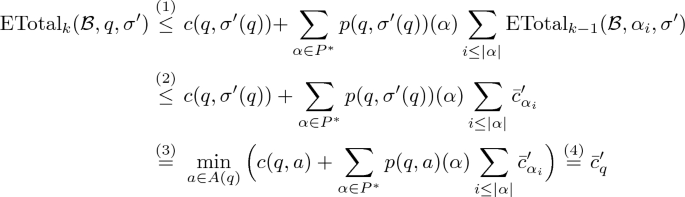
  where (1) follows from the fact that after taking action $\sigma '(q)$ first, there are only $k-1$ steps left of the BMDP $\mathcal{B}$ that would need to be distributed among the offspring $\alpha$ of q somehow. Allowing for $k-1$ steps for each of the entities $\alpha _i$ is clearly an overestimate of the actual cost. (2) follows from the inductive assumption. (3) follows from the definition of $\sigma '$. The last equality, (4), follows from the fact that $\bar{c}'$ is a fixed point of F.

  Finally, for every $q \in P$, from the definition we have $\bar{c}^*_q = \text {ETotal}_{*}(\mathcal{B}, q) \le \text {ETotal}_{*}(\mathcal{B}, q, \sigma ') = \lim _{k\rightarrow \infty } \text {ETotal}_{k}(\mathcal{B}, q, \sigma ')$ and each element of the last sequence was just shown to be $\le \bar{c}'_q$.

• (e) We know that $\bar{x}^{*} = \lim _{k\rightarrow \infty }\bar{x}^k$ exists in ${\widetilde{\mathbb R}}_{\ge 0}^n$ because it is a monotonically non-decreasing sequence (note that some entries may be infinite). In fact we have $\bar{x}^{*} = \lim _{k \rightarrow \infty } F^{k+1}(\bar{0}) = F(\lim _{k \rightarrow \infty } F^{k}(\bar{0}))$, and thus $\bar{x}^{*}$ is a fixed point of F. So from (d) we have $\bar{c}^* \le \bar{x}^*$. At the same time, due to (c), we have $\bar{x}^k \le \bar{c}^*$ for all $k \ge 0$, so $\bar{x}^* = \lim _{k\rightarrow \infty }\bar{x}^k \le \bar{c}^*$ and thus $\lim _{k\rightarrow \infty }\bar{x}^k = \bar{c}^*$.

   $\square$

The following is a simple corollary of Theorem 4.

Corollary 5

In BMDPs, there exists an optimal static control strategy $\sigma ^*$.

Proof

It is enough to pick as $\sigma ^*$, the strategy $\sigma '$ from Theorem 4.d, for $\bar{c}' = \bar{c}^{*}$. We showed there that for all $k \ge 0$ and $q\in P$ we have $\text {ETotal}_k(\mathcal{B},q,\sigma ^*) \le \bar{c}'_q$. So $\text {ETotal}_*(\mathcal{B},q,\sigma ^*) = \lim _{k\rightarrow \infty } \text {ETotal}_k(\mathcal{B},q,\sigma ^*) \le \bar{c}^*_q = \text {ETotal}_*(\mathcal{B},q)$, so in fact $\text {ETotal}_*(\mathcal{B},q,\sigma ^*) = \text {ETotal}_*(\mathcal{B},q)$ has to hold as clearly $\text {ETotal}_*(\mathcal{B},q,\sigma ^*) \ge \text {ETotal}_*(\mathcal{B},q)$.    $\square$

Note that for a BMDPs with a fixed static strategy $\sigma$ (or equivalently BMCs), we have that $F(\bar{x}) = B_\sigma \bar{x}+ \bar{c}_\sigma$, for some non-negative matrix $B_\sigma \in {\mathbb R}_{\ge 0}^{n \times n}$, and a positive vector $\bar{c}_\sigma > 0$ consisting of all one step costs $c(q,\sigma (q))$. We will refer to F as $F_\sigma$ in such a case and exploit this fact later in various proofs.

We now show that $\bar{c}^*$ is in fact essentially a unique fixed point of F.

Theorem 6

If $F(\bar{x}) = \bar{x}$ and $\bar{x}_q < \infty$ for some $q\in P$ then $\bar{x}_q = \bar{c}^*_q$.

Proof

By Corollary 5, there exists an optimal static strategy, denoted by $\sigma ^*$, which yields the finite optimal reward vector $\bar{c}^*$.

We clearly have that $\bar{x}= F(\bar{x}) \le F_{\sigma ^*} (\bar{x})$, because $\sigma ^*$ is just one possible pick of actions for each type rather than the minimal one as in ($\spadesuit$). Furthermore,

$$\begin{aligned} F_{\sigma ^*}(\bar{x})&= B_{\sigma ^*} \bar{x}+ b_{\sigma ^*} \\&\le B_{\sigma ^*}(B_{\sigma ^*} \bar{x}+ b_{\sigma ^*}) + b_{\sigma ^*} \\&= B^2_{\sigma } \bar{x}+ (B_{\sigma ^*} + 1) b_\sigma ^* \\&\le \ldots \le \lim _{k\rightarrow \infty } B^k_{\sigma ^*} \bar{x}+ \Bigl (\sum ^\infty _{k=0} B^k_{\sigma ^*}\Bigr ) b_{\sigma ^*}. \end{aligned}$$

Note that $\bar{c}^* = (\sum ^\infty _{k=0} B^k_{\sigma ^*}) b_{\sigma ^*}$, because

$$ \bar{c}^* = \lim _{k\rightarrow \infty } F^k(\bar{0}) = \lim _{k\rightarrow \infty } F_{\sigma ^*}^k(\bar{0}) = \lim _{k\rightarrow \infty } \sum ^k_{i=0} B^i_{\sigma ^*} b_{\sigma ^*}. $$

Due to Theorem 4.d, we know that $\bar{c}^*_q \le \bar{x}_q < \infty$, so all entries in the q-th row of $B^k_{\sigma ^*}$ have to converge to 0 as $k\rightarrow \infty$, because otherwise the q-th row of $\sum ^\infty _{k=0} B^k_{\sigma ^*}$ would have at least one infinite value and, as a result, the q-th position of $\bar{c}^* = (\sum ^\infty _{k=0} B^k_{\sigma ^*}) b_{\sigma ^*}$ would also be infinite as all entries of $b_{\sigma ^*}$ are positive. Therefore, $\lim _{k\rightarrow \infty } (B^k_{\sigma ^*} \bar{x})_q = 0$ and so

$$ \bar{x}_q \le (\lim _{k\rightarrow \infty } B^k_{\sigma ^*} \bar{x})_q + ((\sum ^\infty _{k=0} B^k_{\sigma ^*}) b_{\sigma ^*})_q = \bar{c}^*_q. $$

The proof is now complete.   $\square$

4 Q-learning

We next discuss the applicability of Q-learning to the computation of the fixed point defined in the previous section.

Q-learning [30] is a well-studied model-free RL approach to compute an optimal strategy for discounted rewards. Q-learning computes so-called Q-values for every state-action pair. Intuitively, once Q-learning has converged to the fixed point, Q(s, a) is the optimal reward the agent can get while performing action a after starting at s. The Q-values can be initialised arbitrarily, but ideally they should be close to the actual values. Q-learning learns over a number of episodes, each consisting of a sequence of actions with bounded length. An episode can terminate early if a sink-state or another non-productive state is reached. Each episode starts at the designated initial state $s_0$. The Q-learning process moves from state to state of the MDP using one of its available actions and accumulates rewards along the way. Suppose that in the i-th step, the process has reached state $s_i$. It then either performs the currently (believed to be) optimal action (so-called exploitation option) or, with probability $\epsilon$, picks uniformly at random one of the actions available at $s_i$ (so-called exploration option). Either way, if $a_i$, $r_i$, and $s_{i+1}$ are the action picked, reward observed and the state the process moved to, respectively, then the Q-value is updated as follows:

$$ Q_{i+1}(s_i,a_i) = (1-\lambda _i) Q_i(s_i,a_i) + \lambda _i (r_i + \gamma \cdot \max _a Q_i(s_{i+1},a)) , $$

where $\lambda _i \in \, ]0,1[$ is the learning rate and $\gamma \in \, ]0,1]$ is the discount factor. Note the model-freeness: this update does not depend on the set of transitions nor their probabilities. For all other pairs s, a we have $Q_{i+1}(s,a) = Q_i(s,a)$, i.e., they are left unchanged. Watkins and Dayan showed the convergence of Q-learning [30].

Theorem 7

(Convergence [30]). For $\gamma < 1$, bounded rewards $r_i$ and learning rates $0 \le \lambda _i < 1$ satisfying:

$$ \sum _{i=0}^{\infty } \lambda _i = \infty ~\text {and} \sum _{i = 0} ^{\infty } \lambda _i^2 < \infty , $$

we have that $Q_i(s, a) \rightarrow Q(s, a)$ as $i \rightarrow \infty$ for all $s, a \in S {\times } A$ almost surely if all (s, a) pairs are visited infinitely often.

However, in the total reward setting that corresponds to Q-learning with discount factor $\gamma = 1$, Q-learning may not converge, or converge to incorrect values. However, it is guaranteed to work for finite-state MDPs in the setting of undiscounted total reward with a target sink-state under the assumption that all strategies reach that sink-state almost surely. The assumption that we make instead is that every transition of BMDP incurs a positive cost. This guarantees that a process that does not terminate almost surely generates an expected infinite reward in which case the Q-learning will coverage (or rather diverge) to $\infty$, so our results generalise these existing results for Q-learning.

We adopt the Q-learning algorithm to minimise cost as follows. Each episode starts at the designated initial state $q_0 \in P$. The Q-learning process moves from state to state of the BMDP using one of its available actions and accumulates costs along the way. Suppose that, in the i-th step, the process has reached state $\alpha$. It then selects uniformly at random one of the entities of $\alpha$, e.g., the j-th one, $\alpha _j$ and either performs the currently (believed to be) optimal action or, with probability $\epsilon$, picks an action uniformly at random among all the actions available for $\alpha _j$. If c and $\beta$ denote the observed cost and entities spawned by this action, respectively, then the Q-value of the pair $\alpha _j$, $a_i$ are updated as follows:

$$ Q_{i+1}(\alpha _j,a_i) = (1-\lambda _i) Q_i(\alpha _j,a_i) + \lambda _i \big (c + \sum _{i=1}^{|\beta |} \min _{a \in A(\beta _i)} Q_i(\beta _i,a)\big ). $$

and all other Q-values are left unchanged. In the next section we show that Q-learning almost surely converges (diverges) to the optimal finite (respectively, infinite) value of $\bar{c}^*$ almost surely under rather mild conditions.

5 Convergence of Q-Learning for BMDPs

We show almost sure convergence of the Q-learning to the optimal values $\bar{c}^*$ in a number of stages. We first focus on the case when all optimal values in $\bar{c}^*$ are finite. In such a case, we show a weak convergence of the expected optimal values for BMCs to the unique fixed-point $\bar{c}^*$, as defined in Sect. 3. To establish this, we show that the expected Q-values are monotonically decreasing (increasing) if we start with Q-values $\kappa \bar{c}^*$ for $\kappa > 1$ ($\kappa < 1$). This convergence from above and below gives us convergence in expectation using the squeeze theorem.

We then establish almost sure convergence to $\bar{c}^*$ by proving a contraction argument, with the extra assumption that the selection of the Q-value to update is done independently at random in each step.

In the next step, we extend this result to BMDPs, first establishing that Q-learning will almost surely converge to the region of the Q-values less than or equal to $\bar{c}^*$. We then show that, when considering the pointwise limes inferior values of the sequences of Q-values, there is no point in that region such that every $\varepsilon$-ball around it has a non-zero probability to be represented in the limes inferior. This establishes that $\bar{c}^*$ is the fixed point the Q-values converge against.

Only at the very end, we show that Q-learning also converges (or rather diverges) to the optimal value even if that value happens to be infinite. We then turn to a type with non-finite optimal value and provide an argument for the divergence to $\infty$ of its corresponding Q-value.

We assume that all the Q-values are stored in a vector Q of size $(|P| \cdot |A|)$. We also use Q(q, a) to refer to the entry for type $q\in P$ and action $a \in A(q)$. We introduce the target for Q operator, T, that maps a Q-values vector Q to:

$$ T(Q)(q,a) = c(q,a) + \sum _{\alpha \in Q^*} p(q,a)(\alpha ) \sum _{i=1}^{|\alpha |} \min _{a_i \in A(\alpha _i)} Q(\alpha _i,a_i) . $$

We call T the ‘target’, because, when the Q(q, a) value is updated, then

$$ \mathbb {E}(Q_{i+1}(q,a)) = (1-\lambda _i) Q_i(q,a) + \lambda _i T(Q_i)(q,a) $$

holds, whereas otherwise $Q_{i+1}(q,a) = Q_i(q,a)$.

Thus, when Q(q, a) is selected for update with a chance of $p_{q,a}$, we have that

5.1 Convergence for BMCs with Finite $\bar{c}^*$

Since BMCs have only one action, we omit mentioning it for ease of notation.

Note that for BMCs, the target for the Q-values is a simple affine function:

$$ T(Q)(q) = c(q) + \sum _{\alpha \in P^*} p(q)(\alpha ) \sum _{i=1}^{|\alpha |} Q(\alpha _i). $$

And it coincides with operator F as defined in Sect. 3. Therefore, due to Theorem 6, T(Q) has a unique fixed point which is $\bar{c}^*$. Moreover, $T(Q) = BQ + \bar{c}$, where B is a non-negative matrix and $\bar{c}$ is a vector of one step costs c(q), which are all positive.

Naturally, applying T to a non-negative vector Q or multiplying it by B are monotone: $Q \ge Q' \rightarrow T(Q) \ge T(Q')$ and $BQ \ge BQ'$. Also, due to the linearity of T, $\mathbb {E}(T(Q)) = T(\mathbb {E}(Q))$ holds, where Q is a random vector.

We now start with a lemma describing the behaviour of Q-learning for initial Q-values when they happen to be equal to $\kappa \bar{c}^*$ for some $\kappa \ge 1$.

Lemma 8

Let $Q_0 = \kappa \bar{c}^*$ for a scalar factor $\kappa \ge 1$. Then the following holds for all $i \in \mathbb N$,

$$ \bar{c}^* \le T(\mathbb {E}(Q_i)) \le \mathbb {E}(Q_{i+1}) \le \mathbb {E}(Q_i), $$

assuming that Q-value to be updated in each step is selected independently at random.

Proof

We show this by induction. For the induction basis $(i=0)$, we have that $\bar{c}^* \le Q_0$ by definition.

As $\bar{c}^*$ is the fixed-point of T, we have $T(\bar{c}^*)=\bar{c}^*$, and the monotonicity of T provides $T(\bar{c}^*) \le T(Q_0)$. At the same time

$$\begin{aligned} T(Q_0) = T(\kappa \bar{c}^*)&= B \kappa \bar{c}^* + \bar{c}\\&= \kappa (B \bar{c}^* + \bar{c}) - \kappa \bar{c}+ \bar{c}\\&= \kappa \bar{c}^* - (\kappa -1) \bar{c}\\&= Q_0 - (\kappa -1) \bar{c}\le Q_0. \end{aligned}$$

This provides $\bar{c}^* \le T(\mathbb {E}(Q_0)) \le \mathbb {E}(Q_0)$. Finally, $T(\mathbb {E}(Q_0)) \le \mathbb {E}(Q_0)$ entails for a learning rate $\lambda _0 \in [0,1]$ that $T(\mathbb {E}(Q_0)) \le \mathbb {E}(Q_{1}) \le \mathbb {E}(Q_0)$ due to ($\heartsuit$).

For the induction step ($i \mapsto i+1$), we use the induction hypothesis

$$ \bar{c}^* \le T(\mathbb {E}(Q_i)) \le \mathbb {E}(Q_{i+1}) \le \mathbb {E}(Q_i). $$

The monotonicity of T and $\bar{c}^* \le \mathbb {E}(Q_{i+1}) \le \mathbb {E}(Q_i)$ imply that $T(\bar{c}^*) \le T(\mathbb {E}(Q_{i+1})) \le T(\mathbb {E}(Q_i))$ holds. With $T(\bar{c}^*) = \bar{c}^*$ (from the fixed point equations) and the induction hypothesis, $\bar{c}^* \le T(\mathbb {E}(Q_{i+1})) \le \mathbb {E}(Q_{i+1})$ follows.

Using $T(\mathbb {E}(Q_{i+1}) )=\mathbb {E}(T(Q_{i+1}))$, this provides $\mathbb {E}(T(Q_{i+1})) \le \mathbb {E}(Q_{i+1})$, which implies with $\lambda _{i+1} \in [0,1]$ that

$$ T(\mathbb {E}(Q_{i+1}))=\mathbb {E}(T(Q_{i+1}))\le \mathbb {E}(Q_{i+2}) \le \mathbb {E}(Q_{i+1}) $$

holds, completing the induction step.    $\square$

By simply replacing all $\le$ with $\ge$ in the above proof, we can get the following for all initial Q-values that happen to be $\kappa \bar{c}^*$ where $\kappa \le 1$:

Lemma 9

Let $Q_0 = \kappa \bar{c}^*$ for a scalar factor $\kappa \in [0,1]$. Then the following holds for all $i \in \mathbb N$, assuming that the Q-value to update in each step is selected independently at random: $\bar{c}^* \ge T(\mathbb {E}(Q_i)) \ge \mathbb {E}(Q_{i+1}) \ge \mathbb {E}(Q_i)$.    $\square$

We now first establish that the distance between Q and $\bar{c}^*$ can be upper bounded by the distance between Q and T(Q) with a fixed linear factor $\mu > 0$.

Lemma 10

There exists a constant $\mu > 0$ such that

$$ \sum _{q \in P}|(Q - T(Q)(q)| \ge \mu \sum _{q \in P}|(Q - \bar{c}^*(q)| $$

when $Q_0 = \kappa \bar{c}^*$.

Proof

We show this for $\kappa > 1$. The proof for $\kappa < 1$ is similar, and there is nothing to show for $\kappa = 1$.

We first consider the linear programme with a variable for each type with the following constraints for some fixed $\delta >0$:

$$ Q \ge \bar{c}^*, T(Q) \le Q, \text {and} \sum _{q \in P}Q(q) = \sum _{q \in P} \bar{c}^*(q) + \delta . $$

An example solution to this constraint system is $Q = (1 + \frac{\delta }{\sum _{q \in P}\bar{c}^*(q)}) \bar{c}^*$.

We then find a solution minimising the objective $\sum _{q \in P}|(Q - T(Q)(p)|$, noting that all entries are non-negative due to the first constraint. This is expressed by adding $2|P|$ constraints

$$\begin{aligned} x_q&\ge Q(q) - T(Q)(q) \\ x_q&\ge T(Q)(q) - Q(q) \end{aligned}$$

and minimising $\sum _{q \in P}x_q$.

As $\bar{c}^*$ is the only fixed-point of T, and $\sum _{q \in P}Q(q) = \sum _{q \in P} \bar{c}^*(q) + \delta$ implies that, for an optimal solution $Q^*$, $Q^* \ne \bar{c}^*$, we have that

$$ \sum _{q \in P} |(Q^* - T(Q^*)(q)| > 0. $$

Due to the constraint $Q \ge \bar{c}^*$, we always have $Q = \bar{c}^* + Q_\varDelta$ for some $Q_\varDelta > \bar{0}$. We can now re-formulate this linear programme to look for $Q_\varDelta$ instead of Q:

$$\begin{aligned} Q_\varDelta&\ge \bar{0},\\ B Q_\varDelta&\le Q_\varDelta , \text {and} \\ \sum _{q \in P} Q_\varDelta (q)&= \delta , \end{aligned}$$

with the objective to minimise $\sum _{q \in P} | ( Q_\varDelta - B Q_\varDelta )(q)|$.

The optimal solution $Q_\varDelta ^*$ to this linear programme gives an optimal value $Q^* = \bar{c}^*+Q_\varDelta ^*$ for the former and, vice versa, the value $Q^*$ for the former provides an optimal solution $Q_\varDelta ^* - \bar{c}^*$ for the latter, and these two solutions have the same value in their respective objective function.

Thus, while the former constraint system is convenient to show that the value of the objective function is positive, the latter constraint system is, except for $\sum _{q \in P} Q_\varDelta (q) =\delta$, linear. This means that any optimal solution for $\delta = \delta _1$ can be obtained from the optimal solution for $\delta = \delta _2$ just by rescaling it by $\delta _1/\delta _2$. It follows that the optimal value of the objective function is linear in $\delta$, e.g., there exists $\mu > 0$ such that its value is $\mu \delta$.    $\square$

We now show that the sequence of Q-values updates converges in expectation to $\bar{c}^*$ when $Q_0 = \kappa \bar{c}^*$.

Lemma 11

Let $Q_0 = \kappa \bar{c}^*$ where $\kappa \ge 0$. Then, assuming that each type-action pair is selected for update with a minimal probability $p_{\min }$ in each step, and that $\sum _{i=0}^\infty \lambda _i = \infty$, then $\lim _{i \rightarrow \infty } \mathbb {E}(Q_i) = \bar{c}^*$ holds.

Proof

We proof this for $\kappa \ge 1$. A similar proof shows this for any $\kappa \in [0,1]$. Lemma 8 provides that all $\mathbb {E}(Q_i)$ satisfy the constraints $\mathbb {E}(Q_i) \ge \bar{c}^*$ and $T(\mathbb {E}(Q_i)) \le \mathbb {E}(Q_i)$.

Let $p_{\min }$ be the smallest probability any Q-value is selected with in each update step. Due to Lemma 10, there is a fixed constant $\mu > 0$ such that

$$\sum _{q \in P} |Q_i (q) - T(Q_i)(q)| \ge \mu \sum _{q \in P} |Q_i(q) - \bar{c}^*(q)| . $$

By taking the expected value of both sides and the fact that $\bar{c}^* \le T(\mathbb {E}(Q_i)) \le \mathbb {E}(Q_{i+1}) \le \mathbb {E}(Q_i)$ due to Lemma 8, we get

$$\sum _{q \in P} \mathbb {E}(Q_i) (q) - T(\mathbb {E}(Q_i))(q) \ge \mu \sum _{q \in P} \mathbb {E}(Q_i)(q) - \bar{c}^*(q),$$

then due to ($\heartsuit$) we have

$$\begin{aligned} \sum _{q \in P} \mathbb {E}(Q_i)(q) - \mathbb {E}(Q_{i+1})(q) \ge \mu p_{\min } \lambda _i \sum _{q \in P} \mathbb {E}(Q_i)(q) - \bar{c}^*(q), \end{aligned}$$

and finally just by rearranging these terms we get

$$\begin{aligned} \sum _{q \in P} \mathbb {E}(Q_{i+1})(q) - \bar{c}^*(q) \le (1-\mu p_{\min } \lambda _i) \sum _{q \in P} \mathbb {E}(Q_i)(q) - \bar{c}^*(q) . \end{aligned}$$

Note that all summands are positive by Lemma 8.

With $\sum _{i=0}^\infty \lambda _i = \infty$, we get that $\sum _{i=0}^\infty \mu p_{\min } \lambda _i = \infty$, because $p_{\min }$ and $\mu$ are fixed positive values. This implies that $\prod _{i=0}^{\infty } (1-\mu p_{\min } \lambda _i) = 0$ and so the distance between $\mathbb {E}(Q_{i})$ and $\bar{c}^*$ converges to 0.    $\square$

Lemma 11 suffices to show convergence of Q-values in expectation.

Theorem 12

When each Q-value is selected for an update with a minimal probability $p_{\min }$ in each step, and $\sum _{i=0}^\infty \lambda _i = \infty$, then $\lim _{i \rightarrow \infty } \mathbb {E}(Q_i) = \bar{c}^*$ holds for every starting Q-values $Q_0 \ge \bar{0}$.

Proof

We first note that none of the entries of $\bar{c}^*$ can be 0. This implies that there is a scalar factor $\kappa \ge 0$ such that $\bar{0}\le Q_0 \le \kappa \bar{c}^*$. As the $Q_i$ are monotone in the entries of $Q_0$, and as the property holds for $Q_0' = \bar{0}= 0 \cdot \bar{c}^*$ and $Q_0'' = \kappa \bar{c}^*$ by Lemma 11, the squeeze theorem implies that it also holds for $Q_0$.    $\square$

Convergence of the expected value is a weaker property than expected convergence, which also explains why our assumptions are weaker than in Theorem 7. With the common assumption of sufficiently fast falling learning rates, $\sum _{i=0}^\infty {\lambda _i}^2 < \infty$, we will now argue that the pointwise limes inferior of the sequence of Q-values almost surely converges to $\bar{c}^*$. This will later allow us to infer convergence of the actual sequence of Q-values to $\bar{c}^*$.

Theorem 13

When each Q-value is selected for update with a minimal probability $p_{\min }$ in each step,

$$ \sum _{i=0}^\infty \lambda _i = \infty ~\text {and} \sum _{i=0}^\infty \lambda _i^2 < \infty , $$

then $\lim _{i \rightarrow \infty } Q_i = \bar{c}^*$ holds almost surely for every starting Q-values $Q_0 \ge \bar{0}$.

Proof

We assume for contradiction that, for some $\widehat{Q} \ne \bar{c}^*$, there is a non-zero chance of a sequence $\{Q_i\}_{i \in \mathbb N_0}$ such that

• $\Vert \widehat{Q}-\liminf _{i \rightarrow \infty } Q_i\Vert _\infty < \varepsilon '$ for all $\varepsilon ' > 0$, and

• there is a type q such that $\widehat{Q}(q) < T(\widehat{Q})(q)$.

Then there must be an $\varepsilon >0$ such that $\widehat{Q}(q)+3 \varepsilon < T(\widehat{Q} - 2 \varepsilon \cdot \bar{1})(q)$. We fix such an $\varepsilon >0$.

Now we have the assumption that the probability of $\Vert \widehat{Q}-\liminf _{n \rightarrow \infty } Q_i\Vert _\infty < \varepsilon$ is positive. Then, in particular, the chance that, at the same time, $\liminf _{i \rightarrow \infty } Q_i > \widehat{Q} - \varepsilon \cdot \bar{1}$ and $\liminf _{i \rightarrow \infty } Q_i < \widehat{Q} + \varepsilon \cdot \bar{1}$, is positive.

Thus, there is a positive chance that the following holds: there exists an $n_\varepsilon$ such that, for all $i>n_\varepsilon$, $Q_i \ge \widehat{Q} - 2 \varepsilon \cdot \bar{1}$. This implies

$$ T(Q_i)(q) \ge T(\widehat{Q} - 2 \varepsilon \cdot \bar{1})(q) > \widehat{Q}(q)+ 3 \varepsilon . $$

Thus, the expected limit value of $Q_i(q)$ is at least $\widehat{Q}(q)+3\varepsilon$, for every tail of the update sequence. Now, we can use $\widehat{Q} - 2\varepsilon$ as a bound on the estimation of the updates in Q-learning as $Q_i \ge \widehat{Q} - 2 \varepsilon \cdot \bar{1}$ holds. At the same time, the variation of the sum of the updates goes to 0 when $\sum {i=0}^\infty \lambda _i^2$ is bounded. Therefore, it cannot be that $\liminf _{i \rightarrow \infty } Q_i < \widehat{Q} + \varepsilon \cdot \bar{1}$ holds; a contradiction.

We note that if, for a Q-values $Q\ge \bar{0}$, there is a $q\in P$ with $Q(q') < \bar{c}^*(q')$, then there is a $q \in P$ with $Q(q) < T(Q)(q)$ and $Q(q) < \bar{c}^*(q)$. This is because, for the Q-values $Q'$ with $Q'(q) = \min \{Q(q),\bar{c}^*(q)\}$ for all $q\in Q$, $Q' < \bar{c}^*$. Thus, there must be a type $q\in P$ such that $\kappa = \frac{Q'(q)}{\bar{c}^*(q)} < 1$ is minimal, and $Q' \ge \kappa \bar{c}^*$. As we have shown before, $T(\kappa \bar{c}^*) = \kappa \bar{c}^* - (\kappa -1) \bar{c}$, such that the following holds:

$$ T(Q)(q) \ge T(Q')(q) \ge T(\kappa \bar{c}^*)(q) = \kappa \bar{c}^*(q) + (1-\kappa ) c(q) > \bar{c}^*(q) = Q(q). $$

Thus, we have that $\liminf _{i \rightarrow \infty } Q_i \ge \bar{c}^*$ holds almost surely. With $\lim _{i \rightarrow \infty } \mathbb {E}(Q_i) = \bar{c}^*$, it follows that $\lim _{i \rightarrow \infty } Q_i = \bar{c}^*$.    $\square$

5.2 Convergence for BMDPs and Finite $\bar{c}^*$

We start with showing that, for BMDPs, the pointwise limes superior of each sequence is almost surely less than or equal to $\bar{c}^*$. We then proceed to show that the limes inferior of a sequence is almost surely $\bar{c}^*$, which together implies almost sure convergence.

Lemma 14

When each Q-value of BMDP is selected for update with a minimal probability $p_{\min }$ in each step, $\sum _{i=0}^\infty \lambda _i = \infty$, $\sum _{i=0}^\infty \lambda _i^2 < \infty$, then $\limsup _{i \rightarrow \infty } Q_i \le \bar{c}^*$ holds almost surely for every starting Q-values $Q_0 \ge \bar{0}$.

Proof

To show the property for the limes superior, we fix an optimal static strategy $\sigma ^*$ that exists due to Corollary 5.

We define an BMC obtained by replacing each type q in the BMDP with $A(q) = \{a_1,\ldots ,a_k\}$, by k types $(q,a_1), \ldots , (q,a_k)$ with one action, where each type $q'$ is replaced by the type-action pair $(q',\sigma ^*(q'))$.

It is easy to see that a type $(q,\sigma ^*(q))$ for the resulting BMC has the same value as the type q and the type-action pair $(q,\sigma ^*(q))$ in the BMDP that we started with.

When identifying these corresponding type-action pairs, we can look at the same sampling for the BMDP and the BMC, leading to sequences $Q_0,Q_1, Q_2, \ldots$ and $Q_0',Q_1', Q_2', \ldots$, respectively, where $Q_0 = Q_0'$.

It is easy to see by induction that $Q_i \le Q_i'$. Considering that $\{Q_i'\}_{i \in \mathbb N}$ almost surely converges to $\bar{c}^*$ by Theorem 13, we obtain our result.    $\square$

Theorem 15

When each Q-value of an BMDP is selected for update with a minimal probability $p_{\min }$, $\sum _{i=0}^\infty \lambda _i = \infty$, $\sum _{i=0}^\infty \lambda _i^2 < \infty$, then $\lim _{i \rightarrow \infty } Q_i = \bar{c}^*$ holds almost surely for every starting Q-values $Q_0 \ge \bar{0}$.

Proof

As a first simple corollary from Lemma 14, we get the same result for the limes inferior (as $\liminf \le \limsup$ must hold).

We now assume for contradiction that, for some vector $\widehat{Q} < \bar{c}^*$, there is a non-zero chance of a sequence $\{Q_i\}_{i \in \mathbb N}$ such that $\Vert \widehat{Q}-\liminf _{n \rightarrow \infty } Q_i\Vert _\infty < \varepsilon '$ for all $\varepsilon ' > 0$.

As $\widehat{Q}$ is below the fixed point of T, there must be one type-action pair $(q,\sigma ^*(q))$ such that $\widehat{Q}(q,\sigma ^*(q)) < T(\widehat{Q})(q,\sigma ^*(q))$ (cf. the proof of Theorem 13). Moreover, there must be an $\varepsilon >0$ such that

$$ \widehat{Q}(q,\sigma ^*(q))+3 \varepsilon < T(\widehat{Q} + 2 \varepsilon \cdot \bar{1})(q,\sigma ^*(q)). $$

We fix such an $\varepsilon >0$.

Now we assume that the probability of $\Vert \widehat{Q}-\liminf _{n \rightarrow \infty } Q_i\Vert _\infty < \varepsilon$ is positive. Then the chance that, simultaneously, $\liminf _{i \rightarrow \infty } Q_i(q,\sigma ^*(q)) > \widehat{Q}(q,\sigma ^*(q)) - \varepsilon$ and $\liminf _{i \rightarrow \infty } Q_i(q,\sigma ^*(q)) < \widehat{Q}(q,\sigma ^*(q)) + \varepsilon$, is positive.

Thus, there is a positive chance that the following holds: there exists an $n_\varepsilon$ such that, for all $i>n_\varepsilon$ we have $Q_i \ge \widehat{Q} - 2 \varepsilon \cdot \bar{1}$. This entails

$$ T(Q_i)(q,\sigma ^*(q)) \ge T(\widehat{Q} - 2 \varepsilon \cdot \bar{1})(q,\sigma ^*(q)) > \widehat{Q}(q,\sigma ^*(q))+ 3 \varepsilon . $$

Thus, the expected limit value of $Q_i(q,\sigma ^*(a))$ is at least $\widehat{Q}(q,\sigma ^*(a))+3\varepsilon$, for every tail of the update sequence. Now, we can use $T(\widehat{Q} - 2\varepsilon \cdot \bar{1})(q,\sigma ^*(a))$ as a bound on the estimation of $T(Q)(q,\sigma ^*(q))$ during the update of the Q-value of the type-action pair $(q,\sigma ^*(q))$. At the same time, the variation of the sum of the updates goes to 0 when $\sum _{i=0}^\infty \lambda _i^2$ is bounded. Therefore, it cannot be that $\liminf _{i \rightarrow \infty } Q_i(q,\sigma ^*(a)) < \widehat{Q}(q,\sigma ^*(a)) + \varepsilon$ holds; a contradiction.    $\square$

5.3 Divergence

We now show divergence of Q(q) to $\infty$ when at least one of the entries of $\bar{c}^*(q)$ is infinite. First due to Theorem 6 and its proof we have that $\bar{c}^* = \sum _{i=0}^\infty B^i \bar{c}$ for some non-negative B and positive $\bar{c}$. Therefore $\bar{c}^*$ is monotonic in B for BMCs. Likewise, the value of $\bar{c}^*$ for a BMDP depends only on the cost function and the expected number of successors of each type spawned: Two BMDPs with same cost functions and the expected numbers of successors have the same fixed point $\bar{c}^*$. Thus, if a type q with one action spawns either exactly one q or exactly one $q'$ with a chance of $50\%$ each, or if it spawns 10 successors of type q and another 10 or type $q'$ with a chance of $5\%$, while dying without offspring with a chance of $95\%$, both lead to identical matrices B and so the same $\bar{c}^*$ (though this difference may impact the performance of Q-learning).

Naturally, raising the number of expected number of successors of any type for any type-action pair strictly raises $\bar{c}^*$, while lowering it reduces $\bar{c}^*$, and for every set of expected numbers, the value of $\bar{c}^*$ is either finite or infinite.

Let us consider a set of parameters at the fringe of finite vs. infinite $\bar{c}^*$, and let us choose them pointwise not larger than the parameters from the BMC or BMDP under consideration. As the fixed point from Sect. 3 is clearly growing continuously in the parameter values, this set of expected successors leads to a $\bar{c}^*$ which is not finite.

We now look at the family of parameter values that lead to $\alpha \in [0,1[$ times the expected successors from our chosen parameter at the fringe between finite and infinite values, and refer to it as the $\alpha$-BMDP. Let also $\bar{c}^*_\alpha$ denote the fixed point for the reduced parameters. As the solution to the fixed point grows continuously, so does $\bar{c}^*_\alpha$. Moreover, if $\bar{c}^*_1 = \lim _{\alpha \rightarrow 1} \bar{c}^*_\alpha$ was finite, then $\bar{c}^*$ would be finite as well, because then $\bar{c}^*_1 = \bar{c}^*$.

Clearly, for all parameters $\alpha \in [0,1[$, the Q-values of an $\alpha$-BMC or $\alpha$-BMDP converge against $\bar{c}^*_{\alpha }$. Thus, the Q-values for the BMC or BMDP we have started with converges against a value, which is at least $\sup _{\alpha \in [0,1[}\bar{c}^*_\alpha$. As this is not a finite value, Q-learning diverges to $\infty$.

6 Experimental Results

We implemented the algorithm described in the previous section in the formal reinforcement learning tool Mungojerrie  [21], a C++-based tool which reads BMDPs described in an extension of the PRISM language [18]. The tool provides an interface for RL algorithms akin to that of [3] and invokes a linear programming tool (GLOP) [22] to compute the optimal expected total cost based on the optimality equations ($\spadesuit$).

6.1 Benchmark Suite

The BMDPs on which we tested Q-learning are listed in Table 1. For each model, the numbers of types in the BMDP, are given. Table 1 also shows the total cost (as computed by the LP solver), which has full access to the BMDP. This is followed by the estimate of the total cost computed by Q-learning and the time taken by learning. The learner has several hyperparameters: $\epsilon$ is the exploration rate, $\alpha$ is the learning rate, and $\mathrm {tol}$ is the tolerance for Q-values to be considered different when selecting an optimal strategy. Finally, ep-l is the maximum episode length and ep-n is the number of episodes. The last two columns of Table 1 report the values of ep-l and ep-n when they deviate from the default values. All performance data are the averages of three trials with Q-learning. Since costs are undiscounted, the value of a state-action pair computed by Q-learning is a direct estimate of the optimal total cost from that state when taking that action.

Table 1. Q-learning results. The default values of the learner hyperparameters are: $\epsilon =0.1$, $\alpha =0.1$, tol$=0.01$, ep-l$=30$, and ep-n$=20000$. Times are in seconds.

Models cloud1 and cloud2 are based on the motivating example given in the introduction. Examples bacteria1 and bacteria2 model the population dynamics of a family of two bacteria [28] subject to two treatments. The objective is to determine which treatment results in the minimum expected cost to extinction of the bacteria population. The protein example models a stochastic Petri net description [19] corresponding to a protein synthesis example with entities corresponding to active and inactive genes and proteins. The example frozenSmall [3] is similar to classical frozen lake example, except that one of the holes result in branching the process in two entities. Entities that fall in the target cell become extinct. The objective is to determine a strategy that results in a minimum number of steps before extinction. Finally, the remaining 5 examples are randomly created BMDP instances.

7 Conclusion

We study the total reward optimisation problem for branching decision processes with unknown probability distributions, and give the first reinforcement learning algorithm to compute an optimal policy. Extending Q-learning is hard, even for branching processes, because they lack a central property of the standard convergence proof: as the value range of the Q-table is not a priori bounded for a given starting table $Q_0$, the variation of the disturbance is not bounded. This looks like a more substantial obstacle than the one Q-learning faces when maximising undiscounted rewards for finite-state MDPs, and it is well known that this defeats Q-learning. So it is quite surprising that we could not only show that Q-learning works for branching processes, but extend these results to branching decision processes, too. Finally, in the previous section, we have demonstrated that our Q-learning algorithm works well on examples of reasonable size even with default hyperparameters, so it is ready to be applied in practice without the need for excessive hyperparameter tuning.

References

Becker, N.: Estimation for discrete time branching processes with application to epidemics. In: Biometrics, pp. 515–522 (1977)
Brázdil, T., Kiefer, S.: Stabilization of branching queueing networks. In: 29th International Symposium on Theoretical Aspects of Computer Science (STACS 2012), vol. 14, pp. 507–518 (2012). https://doi.org/10.4230/LIPIcs.STACS.2012.507
Brockman, G., Cheung, V., Pettersson, L., Schneider, J., Schulman, J., Tang, J., Zaremba, W.: OpenAI Gym. CoRR abs/1606.01540 (2016)
Chen, T., Dräger, K., Kiefer, S.: Model checking stochastic branching processes. In: Rovan, B., Sassone, V., Widmayer, P. (eds.) MFCS 2012. LNCS, vol. 7464, pp. 271–282. Springer, Heidelberg (2012). https://doi.org/10.1007/978-3-642-32589-2_26
Esparza, J., Gaiser, A., Kiefer, S.: A strongly polynomial algorithm for criticality of branching processes and consistency of stochastic context-free grammars. Inf. Process. Lett. 113(10–11), 381–385 (2013)
Etessami, K., Stewart, A., Yannakakis, M.: Greatest fixed points of probabilistic min/max polynomial equations, and reachability for branching Markov decision processes. Inf. Comput. 261, 355–382 (2018). https://doi.org/10.1016/j.ic.2018.02.013
Etessami, K., Stewart, A., Yannakakis, M.: Polynomial time algorithms for branching Markov decision processes and probabilistic min(max) polynomial bellman equations. Math. Oper. Res. 45(1), 34–62 (2020). https://doi.org/10.1287/moor.2018.0970
Etessami, K., Wojtczak, D., Yannakakis, M.: Recursive stochastic games with positive rewards. Theor. Comput. Sci. 777, 308–328 (2019). https://doi.org/10.1016/j.tcs.2018.12.018
Etessami, K., Yannakakis, M.: Recursive Markov chains, stochastic grammars, and monotone systems of nonlinear equations. J. ACM 56(1), 1–66 (2009)
Etessami, K., Yannakakis, M.: Recursive Markov decision processes and recursive stochastic games. J. ACM 62(2), 11:1–11:69 (2015). https://doi.org/10.1145/2699431
Even-Dar, E., Mansour, Y., Bartlett, P.: Learning rates for q-learning. J. Mach. Learn. Res. 5(1) (2003)
Haccou, P., Haccou, P., Jagers, P., Vatutin, V.: Branching processes: variation, growth, and extinction of populations. No. 5 in Cambridge Studies in Adaptive Dynamics, Cambridge University Press (2005)
Harris, T.E.: The Theory of Branching Processes. Springer, Berlin (1963)
Heyde, C.C., Seneta, E.: I. J. Bienaymé: Statistical Theory Anticipated. Springer, Heidelberg (1977). https://doi.org/10.1007/978-1-4684-9469-3
Jo, K.Y.: Optimal control of service in branching exponential queueing networks. In: 26th IEEE Conference on Decision and Control, vol. 26, pp. 1092–1097. IEEE (1987)
Kiefer, S., Wojtczak, D.: On probabilistic parallel programs with process creation and synchronisation. In: Abdulla, P.A., Leino, K.R.M. (eds.) TACAS 2011. LNCS, vol. 6605, pp. 296–310. Springer, Heidelberg (2011). https://doi.org/10.1007/978-3-642-19835-9_28
Kolmogorov, A.N., Sevastyanov, B.A.: The calculation of final probabilities for branching random processes. Doklady Akad. Nauk. U.S.S.R. (N.S.) 56, 783–786 (1947)
Kwiatkowska, M., Norman, G., Parker, D.: PRISM 4.0: verification of probabilistic real-time systems. In: Gopalakrishnan, G., Qadeer, S. (eds.) CAV 2011. LNCS, vol. 6806, pp. 585–591. Springer, Heidelberg (2011). https://doi.org/10.1007/978-3-642-22110-1_47
Munsky, B., Khammash, M.: The finite state projection algorithm for the solution of the chemical master equation. J. Chem. Phys. 124(4), 044104+ (2006)
Nielsen, L.R., Kristensen, A.R.: Markov decision processes to model livestock systems. In: Plà-Aragonés, L.M. (ed.) Handbook of Operations Research in Agriculture and the Agri-Food Industry. ISORMS, vol. 224, pp. 419–454. Springer, New York (2015). https://doi.org/10.1007/978-1-4939-2483-7_19
Perez, M., Somenzi, F., Trivedi, A.: Mungojerrie: formal reinforcement learning (2021). https://plv.colorado.edu/mungojerrie/. University of Colorado Boulder
Perron, L., Furnon, V.: Or-tools (version 7.2) (2019). https://developers.google.com/optimization. Google
Pliska, S.R.: Optimization of multitype branching processes. Manag. Sci. 23(2), 117–124 (1976)
Puterman, M.L.: Markov Decision Processes: Discrete Stochastic Dynamic Programming. Wiley, Hoboken (1994)
Rao, A., Bauch, C.T.: Classical Galton-Watson branching process and vaccination. Int. J. Pure Appl. Math. 44(4), 595 (2008)
Rothblum, U.G., Whittle, P.: Growth optimality for branching Markov decision chains. Math. Oper. Res. 7(4), 582–601 (1982)
Sutton, R.S., Barto, A.G.: Reinforcement Learning: An Introduction, 2nd edn. MIT Press, Cambridge (2018)
Trivedi, A., Wojtczak, D.: Timed branching processes. In: 2010 Seventh International Conference on the Quantitative Evaluation of Systems, pp. 219–228. IEEE (2010)
Udom, A.U.: A Markov decision process approach to optimal control of a multi-level hierarchical manpower system. CBN J. Appl. Stat. 4(2), 31–49 (2013)
Watkins, C.J., Dayan, P.: Q-learning. Mach. Learn. 8(3–4), 279–292 (1992). https://doi.org/10.1007/BF00992698
Watson, H.W., Galton, F.: On the probability of the extinction of families. J. Anthrop. Inst. 4, 138–144 (1874)
Wojtczak, D.: Recursive probabilistic models : efficient analysis and implementation. Ph.D. thesis, University of Edinburgh, UK (2009). http://hdl.handle.net/1842/3217
Author information
Authors and Affiliations
Corresponding author
Editor information
Editors and Affiliations
Rights and permissions
Open Access This chapter is licensed under the terms of the Creative Commons Attribution 4.0 International License (http://creativecommons.org/licenses/by/4.0/), which permits use, sharing, adaptation, distribution and reproduction in any medium or format, as long as you give appropriate credit to the original author(s) and the source, provide a link to the Creative Commons license and indicate if changes were made.
The images or other third party material in this chapter are included in the chapter's Creative Commons license, unless indicated otherwise in a credit line to the material. If material is not included in the chapter's Creative Commons license and your intended use is not permitted by statutory regulation or exceeds the permitted use, you will need to obtain permission directly from the copyright holder.
Copyright information
© 2021 The Author(s)
About this paper
Cite this paper
Hahn, E.M., Perez, M., Schewe, S., Somenzi, F., Trivedi, A., Wojtczak, D. (2021). Model-Free Reinforcement Learning for Branching Markov Decision Processes. In: Silva, A., Leino, K.R.M. (eds) Computer Aided Verification. CAV 2021. Lecture Notes in Computer Science(), vol 12760. Springer, Cham. https://doi.org/10.1007/978-3-030-81688-9_30
Download citation
DOI: https://doi.org/10.1007/978-3-030-81688-9_30
Published:
Publisher Name: Springer, Cham
Print ISBN: 978-3-030-81687-2
Online ISBN: 978-3-030-81688-9
eBook Packages: Computer ScienceComputer Science (R0)