
Abstract
It is a basic idea for the classical theory of Fourier series to express periodic functions as compositions of harmonic waves. This idea can be successfully extended to nonperiodic functions by means of Fourier transforms. However, we will be confronted with a lot of obstacles when we consider \(\mathfrak {L}^p\)-function spaces in the case p > 2.
This is a preview of subscription content, log in via an institution.
Buying options
Tax calculation will be finalised at checkout
Purchases are for personal use only
Learn about institutional subscriptionsNotes
- 1.
I am much indebted to Dunford and Schwartz [7] pp. 281–285, Katznelson [8] pp. 191–200, Kawata [9] II, pp. 96–103, 149–152, [10], [11] pp. 78–86, Loomis [12], Rudin [16, 17] for the contents of this chapter. The classical works cited above are Bohr [4, 5], von Neumann [19], Bochner [2] and Bochner and von Neumann [3].
- 2.
In fact, we note that f(0) = 2 and f(x) ≠ 2 if x ≠ 0. If f(x) = 2, we must have \(\cos x=\cos \pi x=1\). It follows that both \(x=2k\pi \; (k\in \mathbb {Z})\) and \(\pi x=2k\pi \; (k\in \mathbb {Z})\) would have to hold good at the same time. However, it is impossible.
- 3.
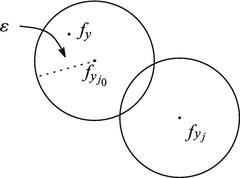
For any ε > 0, there exists some δ > 0 such that
$$\displaystyle \begin{aligned} |f(u)-f(v)|<\frac{\varepsilon}{2} \quad \text{if}\quad |u-v|<\delta. \end{aligned} $$We make a decomposition \(\eta _j(1 \leqq j \leqq J)\) of [0, Λ] so that distances of any two adjacent points are less than δ. y 0 ∈ [0, Λ] is contained in a small interval [η j, η j+1]. Hence
$$\displaystyle \begin{aligned} |f(x-y_0)-f(x-\eta_j)|&<\frac{\varepsilon}{2}. \\ (\text{Note that}\; |(x-y_0)-(x-\eta_j)|&=|y_0-\eta_j|<\delta. ) \end{aligned} $$
This holds good for any \(x \in \mathbb {R}\), and so (9.5) follows.
- 4.
- 5.
- 6.
\(\bar {\mathrm {co}}A\) is the closed convex hull of a set A. coA is the convex hull of A.
- 7.
Select some c n ∈{c 1, c 2, ⋯, c N} such that \(\|(b_1,b_2,\cdots ,b_J)-c_n\|{ }_1<\varepsilon J^{-1}\|f\|{ }_\infty ^{-1}\) and express this c n as
$$\displaystyle \begin{aligned} c_n=(c_{n,1}, c_{n,2}, \cdots ,c_{n,J})=(b_1^{\prime},b_2^{\prime},\cdots,b_J^{\prime}). \end{aligned}$$Then the following evaluation follows.
$$\displaystyle \begin{aligned} \bigg\|\sum_jb_jf_{y_j}(x)-\sum_jc_{n,j}f_{y_j}(x)\bigg\|{}_\infty \leqq \bigg\|\sum_j(b_j-c_{n,j})f_{y_j}(x)\bigg\|{}_\infty =\bigg\|\sum_j(b_j-b_j^{\prime})f_{y_j}(x)\bigg\|{}_\infty <\varepsilon . \end{aligned}$$ - 8.
cf. Appendix C, p. 397.
- 9.
In fact, we have
$$\displaystyle \begin{aligned} \widehat{f_y}(\varphi)&=f_y(\hat{\varphi}) =\frac{1}{\sqrt{2\pi}}\int \int \varphi(\xi)e^{-i\xi x}d\xi f(x-y)dx \\ &=\frac{1}{\sqrt{2\pi}}\int \int \varphi(\xi)e^{-i\xi(y+z)}d\xi f(z)dz \\ &=f(\widehat{\varphi\cdot e^{-i\xi y}})=\hat{f}(\varphi\cdot e^{-i\xi y}) = e^{-i\xi y}\hat{f}(\varphi) \end{aligned} $$for any \(\varphi \in \mathfrak {S}\) by the definition of the Fourier transform of distributions. Hence \(\widehat {f}_y=e^{-i\xi y}\hat {f}\). In the course of computations, f(⋅) and f y(⋅) are tempered distributions defined by the functions f and f y. cf. Appendix C, Sect. C.3, p. 389.
- 10.
We shall give a brief proof. Since g ∈ W(f), there exists a sequence {g n} of functions of the form
$$\displaystyle \begin{aligned} \sum a_k f_{x_k},\; x_k\in\mathbb{R},\; \sum |a_k|\leqq 1 \end{aligned}$$such that ∥g n − g∥∞→ 0 (as n →∞), by Remark 9.1, 1∘. Hence it is easy to see that the sequence of tempered distributions defined by g n’s simply converges to the tempered distribution defined by g. Consequently, \(\hat {g_n}\) also simply converges to \(\hat {g}\) in \(\mathfrak {S}'\) (cf. 2∘ on p. 86). If the support of a function \(\varphi \in \mathfrak {S}\) is contained outside \(\mathrm {supp}\hat {f}\), \(\hat {g}_n(\varphi )=0\) since \(\mathrm {supp}\hat {f}_{x_k}=\mathrm {supp}\hat {f}\). Therefore \(\displaystyle \hat {g}(\varphi )=\lim _{n\rightarrow \infty }\hat {g_n}(\varphi )=0\). We conclude \(\mathrm {supp}\hat {g}\subset \mathrm {supp}\hat {f}\).
- 11.
The Fourier transform of e iξx can be evaluated as in Example 4.9 on p. 85. For any \({\varphi \in \mathfrak {S}}\), we have
$$\displaystyle \begin{aligned}\widehat{e^{i\xi x}}(\varphi)=\int_{-\infty}^\infty e^{i\xi x}\hat{\varphi}(x)dx =\sqrt{2\pi}\varphi(\xi).\end{aligned}$$Hence
$$\displaystyle \begin{aligned} \widehat{e^{i\xi x}}=\sqrt{2\pi}\delta_\xi \end{aligned}$$is derived.
- 12.
Since \(F\in \mathfrak {L}^1\), the mapping \(y\mapsto \tau _y F\;(\mathbb {R}\rightarrow \mathfrak {L}^1)\) is uniformly continuous by Theorem 5.1 (p. 1). It is, of course, continuous at y = 0. Hence there exists some θ > 0, for each ε > 0, such that ∥τ y F − F∥1 < ε provided that |y| < θ. Combining this result and 1∘, we obtain 2∘.
- 13.
Obviously (9.26) holds good if we use f instead of h.
- 14.
It can be verified by
$$\displaystyle \begin{aligned} \eta F(\eta x)\ast c=\int_{\mathbb{R}}\eta F(\eta(x-y))cdy =c\int_{\mathbb{R}}\eta F(\eta&(x-y))dy=c\int_{\mathbb{R}}F(u)du=c \\ &(\text{changing variables: } \eta(x-y)=u ). \end{aligned} $$ - 15.
By definition of W(f), we have 0 ∈ σ(f).
- 16.
Katznelson [8] 2nd edn., pp. 159–160. There is a difference in the explanation of this result between the second edition and the third one. The latter seems to contain a slip.
- 17.
\(\hat {f}\) is the Fourier transform of f in the sense of distribution.
- 18.
\(\hat {f}\) is the Fourier transform of the tempered distribution defined by f.
- 19.
- 20.
\(\hat {f}\), \(\hat {g}_\eta \) are the Fourier transforms of distributions.
- 21.
We use such a notation because we wish to interpret the Fourier transform of f as something like a measure and its value at ξ as the mass at ξ.
- 22.
In the case n = 1, \(P(x)=e^{i\xi _1 x}\) works. Next assume that there exist λ 1, λ 2, ⋯, λ q which satisfy (a) and (b) for ξ 1, ξ 2, ⋯, ξ n−1. Consider ξ 1, ξ 2, ⋯, ξ n. We may assume that
$$\displaystyle \begin{aligned} \xi_n\notin \sum_{h=1}^q\lambda_h\mathbb{Z} \end{aligned}$$for any λ 1, λ 2, ⋯, λ q which satisfy (a) and (b). (Otherwise ξ n is also expressible in the form (b) by using λ 1, λ 2, ⋯λ q.) Define λ by
$$\displaystyle \begin{aligned} \lambda=\xi_n-\sum_{h=1}^q\lambda_hz_h \quad \text{for}\quad z_h \in \mathbb{Z}.\end{aligned}$$Assume that
$$\displaystyle \begin{aligned} \sum_{h=1}^q\theta_h\lambda_h+\theta\lambda=0,\quad \theta_h,\theta\in \mathbb{Q}. \end{aligned}$$If θ = 0, then θ h = 0 (h = 1, 2, ⋯, q) by (a). Hence we may concentrate at the case θ ≠ 0. Since
$$\displaystyle \begin{aligned} \sum_{h=1}^q\theta_h\lambda_h+\theta\lambda=\sum_{h=1}^q\theta_h\lambda_h +\theta\bigg(\xi_n-\sum_{h=1}^q\lambda_hz_h\bigg)=\sum_{h=1}^q(\theta_h-\theta z_h)\lambda_h+\theta\xi_n=0, \end{aligned}$$it is obvious that
$$\displaystyle \begin{aligned} \xi_n=-\sum_{h=1}^q\frac{\theta_h-\theta z_h}{\theta}\lambda_h. \end{aligned}$$Expressing \(\theta _h/\theta =v_h/u_h \; (u_h, v_h\in \mathbb {Z},\, h=1,2,\cdots ,q)\), we denote by u ∗ the least common multiple of u h’s. If we write \(\theta _h/\theta =v_h^*/u^*\), we obtain
$$\displaystyle \begin{aligned} \xi_n=-\sum_{h=1}^q\bigg(\frac{v_h^*}{u^*}-z_h\bigg)\lambda_h=-\sum_{h=1}^q(v_h^*-u^*z_h)\frac{\lambda_h}{u^*}. \end{aligned}$$Furthermore, if we write \(\lambda _h^*=\lambda _h/u^*\;(h=1,2,\cdots, q)\), ξ j’s can be reexpressed as
$$\displaystyle \begin{aligned} \xi_j&=\sum_{h=1}^qu^*A_{j,h}\lambda_h^*,\; j=1,2,\cdots,n-1, \\ \xi_n&=-\sum_{h=1}^q(v_h^*-u^*z_h)\lambda_h^*. \end{aligned} $$Thus \(\lambda _1^*,\lambda _2^*,\cdots ,\lambda _q^*\) satisfy (a) and (b) for ξ 1, ξ 2, ⋯, ξ n−1 and also
$$\displaystyle \begin{aligned} \xi_n\in \sum_{h=1}^q\lambda_h^*\mathbb{Z}. \end{aligned}$$This contradicts our assumption. Hence θ must be zero.
- 23.
The proof of (i)⇔(ii) is due to Kawata [11] pp. 80–82.
- 24.
A function of the form
$$\displaystyle \begin{aligned}f(x)=\sum_{j=1}^na_je^{-i\xi_j u}\quad (\xi_j\in \mathbb{R}) \end{aligned}$$is called a trigonometric polynomial. Any trigonometric polynomial is almost periodic.
- 25.
This observation is based upon Maruyama [15].


References
Billingsley, P.: Convergence of Probability Measures. Wiley, New York (1968)
Bochner, S.: Beiträge zur Theorie der fastperiodischen Funktionen, I, II. Math. Ann. 96, 119–147, 383–409 (1927)
Bochner, S., von Neumann, J.: Almost periodic functions in a group, II. Trans. Amer. Math. Soc. 37, 21–50 (1935)
Bohr, H.: Zur Theorie der fastperiodischen Funktionen. I–III. Acta Math. 45, 29–127 (1925); 46, 101–214 (1925); 47, 237–281 (1926)
Bohr, H.: Fastperiodische Funktionen. Springer, Berlin (1932)
Dudley, R.M.: Real Analysis and Probability. Wadsworth and Brooks, Pacific Grove (1988)
Dunford, N., Schwartz, J.T.: Linear Operators, Part 1, Interscience, New York (1958)
Katznelson, Y.: An Introduction to Harmonic Analysis, 3rd edn. Cambridge University Press, Cambridge (2004)
Kawata, T.: Ohyo Sugaku Gairon (Elements of Applied Mathematics). I, II. Iwanami Shoten, Tokyo (1950, 1952) (Originally published in Japanese)
Kawata, T.: On the Fourier series of a stationary stochastic process, I, II. Z. Wahrsch. Verw. Gebiete, 6, 224–245 (1966); 13, 25–38 (1969)
Kawata, T.: Teijo Kakuritsu Katei (Stationary Stochastic Processes). Kyoritsu Shuppan, Tokyo (1985) (Originally published in Japanese)
Loomis, L.: The spectral characterization of a class of almost periodic functions. Ann. Math. 72, 362–368 (1960)
Malliavin, P.: Integration and Probability. Springer, New York (1995)
Maruyama, T.: Sekibun to Kansu-kaiseki (Integration and Functional Analysis). Springer, Tokyo (2006) (Originally published in Japanese)
Maruyama, T.: Fourier analysis of periodic weakly stationary processes. A note on Slutsky’s observation. Adv. Math. Econ. 20, 151–180 (2016)
Rudin, W.: Weak almost periodic functions and Fourier–Stieltjes transforms. Duke Math. J. 26, 215–220 (1959)
Rudin, W.: Fourier Analysis on Groups. Interscience, New York (1962)
Stromberg, K.R.: An Introduction to Classical Real Analysis. American Mathematical Society, Providence (1981)
von Neumann, J.: Almost periodic functions in a group, I. Trans. Amer. Math. Soc. 36, 445–492 (1934)
Author information
Authors and Affiliations
Rights and permissions
Copyright information
© 2018 Springer Nature Singapore Pte Ltd.
About this chapter

Cite this chapter
Maruyama, T. (2018). Almost Periodic Functions and Weakly Stationary Stochastic Processes. In: Fourier Analysis of Economic Phenomena. Monographs in Mathematical Economics, vol 2. Springer, Singapore. https://doi.org/10.1007/978-981-13-2730-8_9
Download citation
DOI: https://doi.org/10.1007/978-981-13-2730-8_9
Published:
Publisher Name: Springer, Singapore
Print ISBN: 978-981-13-2729-2
Online ISBN: 978-981-13-2730-8
eBook Packages: Mathematics and StatisticsMathematics and Statistics (R0)