The Clean Development Mechanism

Abstract

This chapter is dedicated to the Clean Development Mechanism (CDM), and more particularly to the secondary Certified Emissions Reductions (CER) originated under these project mechanisms. Indeed, secondary CERs are valid for compliance within the European trading system up to 13.4% on average. Following a review of the main characteristics of CER contracts and price development, we study the relationship between EUAs and CERs in vector autoregressive and cointegration models. Then, we identify the main CER price drivers based on the Zivot-Andrews structural break tests and regression analysis. Finally, we discuss the main reasons behind the existence of the CER-EUA spread, and highlight the possibilities to benefit from arbitrage opportunities. The Appendix shows how to represent the interactions between EUAs and CERs in a Markov regime-switching environment.

Appendix: Markov Regime-Switching Modeling with EUAs and CERs

We recall briefly here the basic framework behind Markov-switching models, as it has already been introduced in Chap. 3.

Consider an n-dimensional vector y _t ≡(y _1t ,…,y _nt )′ which is assumed to follow a VAR(p) with parameters:

$${{\mathbf{y}}_{t}}=\mathbf{\mu }({{s}_{t}})+\sum\limits_{i=1}^{p}{{{\phi }_{i}}({{s}_{t}}){{y}_{t-i}}+{{\varepsilon }_{t}}}$$

(4.26)

$${{\mathbf{\varepsilon }}_{\mathbf{t}}}\sim \mathcal{N}\left( \text{0,}\Sigma \text{(}{{s}_{t}}) \right)$$

(4.27)

where the parameters for the conditional expectation μ(s _t ) and φ _i (s _t ), i=1,…,p, as well as the variances and covariances of the error terms ε _t in the matrix ∑(s _t ) all depend upon the state variable s _t which can assume a number q of values (corresponding to different regimes).

The model is estimated based on Gaussian maximum likelihood with S _t =1,2. By setting S=[1 1], both the autoregressive coefficients and the model’s variance are switching according to the transition probabilities.

Next, we apply this modelling framework to the time series of EUAs and CERs from March 2007 to March 2009. Thus, we obtain a two-regime Markov-switching VAR.

The estimation results are shown in Table 4.19. The statistically significant coefficients of the two means μ show the presence of switches between high-/low-growth periods. During expansion, output growth per month is equal to 0.03% on average. The time series is likely to remain in the expansionary phase with an estimated probability equal to 91%. Regime 1 is assumed to last 11 days on average. During recession, the average growth rate is equal to −0.05%. The probability that it will stay in recession is equal to 80%. The average duration of Regime 2 is equal to 5 days. According to the ergodic probabilities, the time series would spend 60% (40%) of the time spanned by the data sample in Regime 1 (Regime 2).

Table 4.19 Estimation results of the two-regime Markov-switching VAR for EUAs and CERs

Interestingly, other coefficient estimates suggest that EUAs have several statistically significant effects on CERs: during Regime 1 (as φ ₁=0.19 and φ ₂=0.07 are significant at the 5% level), and during Regime 2 (as φ ₁=−0.39 and φ ₂=0.16 are significant at the 1% level). Therefore, these results confirm the insights by Chevallier [3, 4] concerning the significant impact of EUAs on CERs, since the EU ETS is the most developed emissions market in the world to date. Concerning CERs, we can notice that they impact EUAs both during expansionary (as φ ₁=0.70 is significant at the 1% level) and recessionary (as φ ₁=−0.50 is significant at the 5% level) phases.

The smoothed and regime transition probabilities are shown in, respectively, Figs. 4.15 and 4.16. They reveal essentially two states in the carbon futures markets: low-growth periods during April 2007 and April–December 2008, and high-growth periods during May 2007–May 2008 and January 2009–June 2009. These main switches from one regime to another seem to occur during compliance events or major changes in the underlying business cycle (with the entry of world economies into the recession in 2008), which affect the trading of CO₂ assets.

Fig. 4.15

Smoothed transition probabilities estimated from the two-regime Markov-switching VAR for EUAs and CERs

Fig. 4.16

Regime transition probabilities estimated from the two-regime Markov-switching VAR for EUAs and CERs

The diagnostic tests are shown in Table 4.20. The upper panel reports the results of three diagnostic tests. The first is a test of the Markov-switching model against the simple nested null hypothesis that the data follow a geometric random walk with i.i.d. innovations. Note M the p-value from the LR test:

$$\operatorname{Prob}[\mathit{LR}(q^{*})]>M=\operatorname{Prob}(\chi^2_d>M)+ \frac{VM^{(d-1)/2}e^{-M/2} 2^{-d/2}}{\varGamma(d/2)}$$

(4.28)

where Prob (LR(q ^∗)>M|H ₀) is the upper bound critical value, LR is the likelihood ratio statistic, q ^∗ is the vector of transition probabilities $(q^{*}=\arg\max Ln L(q) |H_{1})$ and d is the number of restrictions under the null hypothesis.

Table 4.20 Diagnostic tests of the two-regime Markov-switching VAR for EUAs and CERs

In Table 4.20, this adjustment produces a LR statistic equal to 25.98. We reject the random walk at the 0.1 percent level. We conclude that the relationship is better described by a two-regime Markov-switching model than by the random walk model.

The second test reported in Table 4.20 is for symmetry of the Markov transition matrix, which implies symmetry of the unconditional distribution of the growth rates. This test examines the maintained hypothesis that p (the probability of being in a high-growth state or boom) equals q (the probability of being in a low-growth state or depression) against the alternative that p<q. Table 4.20 reports statistics that are asymptotically standard normal under the null. We reject the hypothesis of symmetry at the 5% level.

Third, Ang and Bekaert (2002, [1]) set out a formal definition of and a test for regime classification. They argue that a good regime switching model should be able to classify regimes sharply. Weak regime inference implies that the regime-switching model cannot successfully distinguish between regimes from the behavior of the data, and may indicate misspecification. To measure the quality of regime classification, we therefore use Ang and Bekaert’s (2002 [1]) Regime Classification Measure (RCM) defined for two states as:

$$\mathit{RCM}=400 \times\frac{1}{T} \sum_{t=1}^{T}p_t (1-p_t) $$

(4.29)

where the constant serves to normalize the statistic to be between 0 and 100, and p _t denotes the ex-post smoothed regime probabilities. Good regime classification is associated with low RCM statistic values. A value of 0 indicates that the two-regime model is able to perfectly discriminate between regimes, whereas a value of 100 indicates that the two-regime model simply assigns each regime a 50% chance of occurrence throughout the sample. Consequently, a value of 50 is often used as a benchmark (see Chan et al. (2011, [2]) for instance).

Adopting this definition to the current context, the RCM 2-State statistic is equal to 38.61 in Table 4.20. It is substantially below 50, consistent with the existence of two regimes. It is very interesting that our estimated Markov-switching model has classified the two regimes extremely well.

Finally, Table 4.20 reports the distributional characteristics for the Markov-switching processes implied by the estimates in Table 4.19. We conclude that the Markov-switching model produces both the degree of skewness and the amount of kurtosis that are present in the original data.

Overall, the Markov-switching modelling brings us new insights as to when market shocks occur, and actually impact the EUA and CER futures price series. The results show that significant interactions exist between the two markets, especially during periods of economic recession when the market trends are destabilised.

4.1.1 Problems

Problem 4.1

(The EUA-CER Spread)

• (a) Consider the time-series in Fig. 4.17: briefly describe the variables that you observe, as well as their behaviour. What are the differences between the two panels?

  Fig. 4.17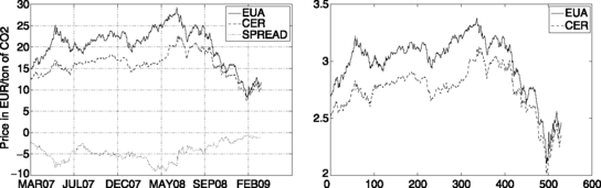

  

  Raw time-series (left panel) and natural logarithms (right panel) of the ECX EUA December 2008/2009 Futures and Reuters CER Price Index from March 9, 2007 to March 31, 2009

• (b) Consider the descriptive statistics in Table 4.21: briefly comment on the descriptive statistics that you observe for each variable.

  Table 4.21 Summary Statistics for the Raw Time Series and Natural Logarithms

  In what follows, the ECX EUA December 2008/2009 and Reuters CER Price Index Raw Series are expressed in natural logarithms.

• (c) Comment on Tables 4.22 and 4.23: which cointegration space can you identify, given a 5% significance level? Provide detailed comments as to which statistics you use, and how you to read these tables.

  Table 4.22 Cointegration Rank: Maximum Eigenvalue Statistic

  Table 4.23 Cointegration Rank: Trace Statistic

• (d) Comment on Tables 4.24, 4.25 and 4.26: based on your conclusion in Question (c), interpret the following Error Correction Model.

  Table 4.24 Cointegration Vector

  Table 4.25 Model Weights

  Table 4.26 VECM with r=1

  In what follows, the ECX EUA December 2008/2009 and Reuters CER Price Index Raw Series are expressed in log-returns.

• (e) Consider the time-series in Fig. 4.18: briefly describe the variables that you observe, and their behaviour. What are the differences compared to Fig. 4.17?

  Fig. 4.18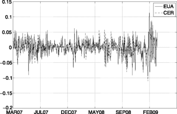

  

  Logreturns of the ECX EUA December 2008/2009 Futures and Reuters CER Price Index from March 9, 2007 to March 31, 2009

• (f) Consider the descriptive statistics in Table 4.27: briefly comment on the descriptive statistics that you observe for each variable.

  Table 4.27 Summary Statistics for the Log-Returns

  You are given the following information:

  • Optimal lag selection: AIC(n)=4, HQ(n)=1, SC(n)=1, FPE(n)=4.

  • p-value of the Portmanteau test < 5% for VAR(1) residuals.

• (g) Comment on Tables 4.28 and 4.29: provide detailed comments of the static VAR analysis for both variables.

  Table 4.28 VAR(4) Model Results for the EUA Variable

  Table 4.29 VAR(4) Model Results for the CER Variable

• (h) Comment on Table 4.30: analyze the diagnostic tests for the VAR(4) model. Can you conclude that the model is well-specified?

  Table 4.30 Diagnostic tests of VAR(4) Model

• (i) Comment on Table 4.31: what can you conclude concerning the Granger causality tests?

  Table 4.31 Granger Causality Tests

• (j) Consider the time-series in Fig. 4.19: briefly comment on the impulse response functions that you observe for each variable. Given your analysis in Questions (c) to (i), which Cholesky decomposition has been chosen to compute these graphs?

  Fig. 4.19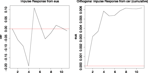

  

  Impulse responses from EUA to CER (left panel) and from CER to EUA (right panel) Variables of the VAR(4) Model

  In what follows, the GARCH(p,q) model with a Gaussian conditional probability distribution has been estimated by Quasi-Maximum Likelihood with the BHHH algorithm.

• (k) Comment on Table 4.32: provide detailed comments for each parameter of the GARCH(p,q) model.

  Table 4.32 GARCH estimates for the CER-EUA Spread

• (l) Comment on Fig. 4.20: what can you conclude with respect to the autocorrelation structure of GARCH estimates?

  Fig. 4.20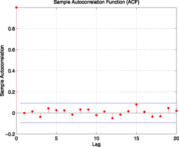

  

  GARCH(1, 1) model autocorrelation of squared logreturns of the CER-EUA Spread

• (m) Consider the time series in Fig. 4.21: as a diagnostic check of these estimates, what can you conclude from Fig. 4.21?

  Fig. 4.21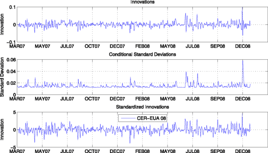

  

  GARCH(1, 1) model of the CER-EUA Spread innovations (top panel), conditional standard deviations (middle panel) and standardized innovations (bottom panel)

References

Ang A, Bekaert G (2002) Regime switches in interest rates. J Bus Econ Stat 20:163–182
Chan KF, Treepongkaruna S, Brooks R, Gray S (2011) Asset market linkages: evidence from financial, commodity and real estate assets. J Bank Finance 35:1415–1426
Chevallier J (2010) EUAs and CERs: vector autoregression, impulse response function and cointegration analysis. Econ Bull 30:558–576
Chevallier J (2011) Anticipating correlations between EUAs and CERs: a dynamic conditional correlation GARCH model. Econ Bull 31:255–272
Collin-Dufresne P, Goldstein RS, Spencer Martin J (2001) The determinants of credit spread changes. J Finance 56:2177–2202
Engle R (1982) Autoregressive conditional heteroskedasticity with estimates of the variance of United Kingdom inflation. Econometrica 50:987–1007
Hamilton JD (1996) Time series analysis, 2nd edn. Princeton University Press, Princeton
Johansen S (1988) Statistical analysis of cointegration vectors. J Econ Dyn Control 12:231–254
Johansen S, Juselius K (1990) Maximum likelihood estimation and the demand for money inference on cointegration with application. Oxf Bull Econ Stat 52:169–210
Johansen S (1991) Estimation and hypothesis testing of cointegration vectors in Gaussian vector autoregressive models. Econometrica 59:1551–1580
Johansen S (1992) Cointegration in partial systems and the efficiency of single-equation analysis. J Econom 52:389–402
Lütkepohl H, Saikkonen P, Trenkler C (2004) Testing for the cointegrating rank of a VAR with level shift an unknown time. Econometrica 72:647–662
Lütkepohl H (2006) New introduction to multiple time series analysis. Springer, New York/Dordrecht/Heidelberg/London
Madhavan A (2000) Market microstructure: a survey. J Financ Mark 3:205–258
Mansanet-Bataller M, Chevallier J, Herve-Mignucci M, Alberola A (2011) EUA and sCER phase II price drivers: unveiling the reasons for the existence of the EUA-sCER spread. Energy Policy 39:1056–1069
Perron P (1989) The great crash, the oil price shock, and the unit root hypothesis. Econometrica 57:1361–1401
Pfaff B (2008) Analysis of integrated and cointegrated time series with R. Springer, New York/Dordrecht/Heidelberg/London
Pinho C, Madaleno M (2011) CO2 emission allowances and other fuel markets interactions. Environ Econ Policy Stud 13:259–281
Ploberger W, Kramer W (1992) The CUSUM test with OLS residuals. Econometrica 60:271–285
Sims CA (1980) Macroeconomics and reality. Econometrica 48:1–48
Trenkler C (2003) A new set of critical values for systems cointegration tests with a prior adjustment for deterministic terms. Econ Bull 3:1–9
Zivot E, Andrews DWK (1992) Further evidence on the great crash, the oil-price shock, and the unit-root hypothesis. J Bus Econ Stat 10:251–270
Author information
Authors and Affiliations
Corresponding author