Machine Scheduling

Abstract

The subject of this chapter is the allocation of jobs (or tasks) to processors (or machines). These terms should be understood in the widest possible sense: in the case of a doctor treating patients the doctor is the processor and the patients represent the tasks, in the case of a tax auditor the auditor is the processor (or the “machine”), while the individual cases are the tasks to be processed. This allocation is to be made so as to optimize some objective. We will discuss a number of these objectives below.

Exercises

Problem 1 (single- and parallel machine scheduling)

A machine scheduling problem has ten jobs with given processing times of 3, 1, 4, 1, 5, 9, 2, 6, 5, and 3 h, respectively.

• (a) Assume that the jobs are to be performed on a single machine and that the objective is to minimize mean flow time, find an optimal schedule and draw the corresponding Gantt chart.

• (b) Assume that due dates for the ten jobs are given as 14, 4, 10, 19, 40, 32, 13, 31, 7, and 26 h, respectively. Use the earliest due date algorithm to find a schedule that minimizes the maximal lateness L _max . Show the corresponding Gantt chart. What is the minimal value of L _max , and for which job does it occur? Which jobs are late?

• (c) Assume that there are two parallel machines to process the jobs. Trying to minimize the schedule length, schedule the jobs using the LPT algorithm. Display the corresponding Gantt chart. What is the performance ratio?

• (d) Given two parallel machines as under (c), what is the schedule that minimizes the mean flow time? Display the corresponding Gantt chart.

• (e) Reconsider questions (c) and (d) given that there are now three rather than two parallel machines.

Solution

• (a) Assuming ready times r _j  = 0, the mean flow time is F is minimized by the shortest processing time (SPT) algorithm. The sequence of jobs is T ₂, T ₄, T ₇, T ₁, T ₁₀, T ₃, T ₅, T ₉, T ₈, and T ₆. The corresponding Gantt chart is shown in Fig. 8.11.

  Fig. 8.11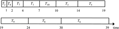

  

  Optimal schedule for Problem 1(a)

  The minimal mean flow time for this schedule is then F = $\tfrac{1}{{10}}(1 + 2 + 4 + 7 +... + 30 + 39) = 15.$ Since T ₁ and T ₁₀ both have processing times of 3 h each, they may be swapped in the optimal schedule, thus creating alternative optimal solutions. A similar argument applies to the pairs T ₂ and T ₄, and T ₅ and T ₉.

• (b) Using the EDD algorithm, we obtain the optimal schedule shown in Fig. 8.12.

  Fig. 8.12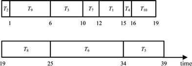

  

  Optimal schedule for Problem 1(b)

  It turns out that task T ₁ is late by 1 h and task T ₆ is late by 2 h. All other tasks are finished on time (but T ₃ only just). The lateness L _max therefore equals 2 h, obtained for T ₆.

• (c) With two machines P1 and P2, the longest processing time LPT Algorithm minimizes the makespan Cmax.

  The makespan is 20 h. In the schedule shown in Fig. 8.13, one of the machines is idle for 1 h.

  Fig. 8.13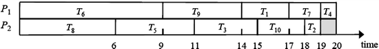

  

  Optimal schedule for Problem 1(c)

• (d) With two machines, find a schedule that minimizes the mean flow time. The Gantt chart is shown in Fig. 8.14.

  Fig. 8.14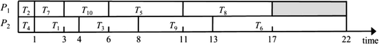

  

  Optimal schedule for Problem 1(d)

  The schedule length is 22 h and the mean flow time is F = $\tfrac{1}{{10}}(1 + 1 + 3 + 4 +... + 17 + 22) = 8.6$, and one processor is idle for 5 h. Since the schedule is optimal, the performance ratio equals 1.

• (e) With three machines, we use the LPT rule as a heuristic to minimize C _max . The Gantt chart is shown in Fig. 8.15.

  Fig. 8.15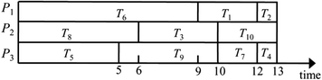

  

  Optimal schedule for Problem 1(e)

The schedule has a makespan of 13 h. Since there is idle time, the schedule must be optimal. Using the algorithm for minimizing mean flow time, we obtain the schedule shown in Fig. 8.16.

Fig. 8.16

Minimizing mean flow time for Problem 1(c)

The schedule length is 18 h and the mean flow time is F = 6.6. Note that there is significant idle time.

Problem 2: (Parallel machine scheduling with preemption)

Consider Example 5 in Sect. 8.3.

• (a) Using the original data, apply the Wrap-Around Rule to find a schedule that minimizes makespan, assuming that preemption is allowed and that there are three, rather than two, processors.

• (b) Consider again the example as under (a). Using the increased processing time of job T ₉, solve the problem with two, rather than three, processors.

Solution

• (a) First, we compute $C_{{\max }}^{*} = \max \left\{ {\mathop{{\max }}\limits_{{1 \leq j \leq 11}} \{ {p_j}\}, \frac{1}{3} \sum\limits_{{j = 1}}^{{11}} {{p_j}} } \right\} = \max \{ {p_9}, \frac{1}{3} (76)\} = { \max }\left\{ {{14},{ 25} \frac{1}{3} } \right\}{ } = { 25} \frac{1}{3}$. Using the Wrap-Around Rule we then obtain the schedule displayed in the Gantt chart in Fig. 8.17.

  Fig. 8.17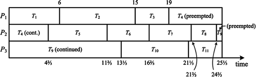

  

  Schedule for Problem 2(a)

  An implementation of this schedule would start T ₄ on P ₂, preempt it at $t = {4} \frac{2}{3}$ and then resume T ₄ on P ₁ at time t = 19. Task T ₉ then starts at P ₃ at t = 0 and is then preempted at $t = {13} \frac{1}{3}$, after which it resumes at $t = {24} \frac{2}{3}$ on P ₂.

• (b) We now find $C_{{\max }}^{*} = \max \{ 34,\raise.5ex\hbox{$\scriptstyle 1$}\kern-.1em/ \kern-.15em\lower.25ex\hbox{$\scriptstyle 2$} (96)\} = 48$, and the Wrap-Around Rule generates the schedule shown in Fig. 8.18.

  Fig. 8.18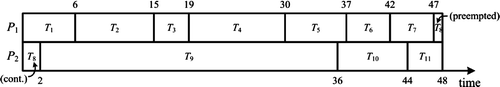

  

  Schedule for Problem 2(b)

For a practical implementation of this schedule, task T ₈ will be started on processor P ₂ at time t = 0, will be preempted at t = 2, and then resumed on P ₁ at time t = 47.

Problem 3 (open shop and flow shop scheduling)

In a hospital laboratory, there are two machines testing patient blood samples. Table 8.5 shows the number of minutes required on each machine to process the samples.

Table 8.5 Data for problem 3

• (a) Assume that the order of processing the blood samples on the two machines is arbitrary. Schedule the testing on the two machines so as to minimize the schedule length. Display the optimal schedule in a Gantt chart. Indicate the schedule length as well as the idle time.

• (b) Assume now that all blood samples must be processed on P ₁ before they can be processed on P ₂. Redo part (a) with these new assumptions.

• (c) Are the optimal schedules in (a) and (b) unique? Discuss. There is no need to display Gantt charts.

Solution

• (a) The LAPT algorithm is used to obtain the optimal schedule shown in Fig. 8.19.

  Fig. 8.19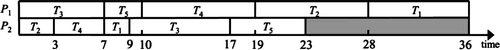

  

  Optimal schedule for Problem 3(a)

  The minimal schedule length is C _max  = 36 min. There is no idle time on P ₁, while P ₂ is idle at the end for 13 min. This is an open shop model.

• (b) Johnson’s rule is used to obtain the optimal schedule shown in Fig. 8.20.

  Fig. 8.20

  

  Optimal schedule for Problem 3(b)

  The minimal schedule length is now C _max  = 38 min. Processor P ₁ has an idle time of 2 min at the very end of the schedule, whereas P ₂ has five separate idle time periods, totaling 15 min. This is a flow shop model.

• (c) In (a), tasks T ₂ and T ₄ could swap positions in the schedule of P ₁ (and on P₂ for that matter) without consequences regarding the schedule length. There are several other changes that would not destroy optimality. In (b), tasks T ₂ and T ₄ could also swap positions on P ₁, necessitating modifications on processor P ₂.