Failure is Not an Option

Abstract

We define the exceptional translation, a syntactic translation of the Calculus of Inductive Constructions (CIC) into itself, that covers full dependent elimination. The new resulting type theory features call-by-name exceptions with decidable type-checking and canonicity, but at the price of inconsistency. Then, noticing parametricity amounts to Kreisel’s realizability in this setting, we provide an additional layer on top of the exceptional translation in order to tame exceptions and ensure that all exceptions used locally are caught, leading to the parametric exceptional translation which fully preserves consistency. This way, we can consistently extend the logical expressivity of CIC with independence of premises, Markov’s rule, and the negation of function extensionality while retaining $\eta$-expansion. As a byproduct, we also show that Markov’s principle is not provable in CIC. Both translations have been implemented in a Coq plugin, which we use to formalize the examples.

1 Introduction

Monadic translations constitute a canonical way to add effects to pure functional languages [1]. Until recently, this technique was not available for type theories such as $\mathrm {CIC}$ because of complex interactions with dependency. In a recent paper [2], we have presented a generic way to extend the monadic translation to dependent types, using the weaning translation, as soon as the monad under consideration satisfies a crucial property: being self-algebraic. Indeed, in the same way that the universe of types ${\square }_{i}$ is itself a type (of a higher universe) in type theory, the type of algebras of a monad

needs to be itself an algebra of the monad to allow a correct translation of the universe. However, in general, the weaning translation does not interpret all of $\mathrm {CIC}$ because dependent elimination needs to be restricted to linear predicates, that is, those that are intuitively call-by-value [3]. In this paper, we study the particular case of the error monad, and show that its weaning translation can be simplified and tweaked so that full dependent elimination is valid.

This exceptional translation gives rise to a novel extension of $\mathrm {CIC}$ with new computational behaviours, namely call-by-name exceptions.¹ That is, the type theory induced by the exceptional translation features new operations to raise and catch exceptions. This new logical expressivity comes at a cost, as the resulting theory is not consistent anymore, although still being computationally relevant. This means that it is possible to prove a contradiction, but, thanks to a weak form of canonicity, only because of an unhandled exception. Furthermore, the translation allows us to reason directly in $\mathrm {CIC}$ on terms of the exceptional theory, letting us prove, e.g., that assuming some properties on its input, an exceptional function actually never raises an exception. We thus have a sound logical framework to prove safety properties about impure dependently-typed programs.

We then push this technique further by noticing that parametricity provides a systematic way to describe that a term is not allowed to produce uncaught exceptions, bridging the gap between Kreisel’s modified realizability [4] and parametricity inside type theory [5]. This parametric exceptional translation ensures that no exception reaches toplevel, thus ensuring consistency of the resulting theory. Pure terms are automatically handled, while it is necessary to show parametricity manually for terms internally using exceptions. We exploit this computational extension of $\mathrm {CIC}$ to show various logical results over $\mathrm {CIC}$.

Contributions

• We describe the exceptional translation, the first monadic translation for the error monad for $\mathrm {CIC}$, including strong elimination of inductive types, resulting in a sound logical framework to reason about impure dependently-typed programs.

• We use parametricity to extend the exceptional translation, getting a consistent variant dubbed the parametric exceptional translation.

• We show that Markov’s rule is admissible in $\mathrm {CIC}$.

• We show that definitional ${\eta }$-expansion together with the negation of function extensionality is admissible in $\mathrm {CIC}$.

• We show that there exists a syntactical model of $\mathrm {CIC}$ that validates the independence of premises (which is known to be generally not valid in intuitionistic logic [6]) and use it to recover the recent result of Coquand and Mannaa [7], i.e., that Markov’s principle is not provable in $\mathrm {CIC}$.

• We provide a Coq plugin² that implements both translations and with which we have formalized all the examples.

Plan of the Paper. In Sect. 2, we describe the exceptional translation and the resulting new computational principles arising from it. In Sect. 3, we present the parametric variant of the exceptional translation. Section 4 is devoted to the various logical results resulting from the parametric exceptional translations. In Sect. 5, we discuss possible extensions of the translation with negative records and an impredicative universe. Section 6 describes the Coq plugin and illustrates its use on a concrete example. We discuss related work in Sect. 7 and conclude in Sect. 8.

Fig. 1.

Typing rules of ${\mathrm {CC}}_{\omega }$

2 The Exceptional Translation

We define in this section the exceptional translation as a syntactic translation between type theories. We call the target theory $\mathcal {T}$, upon which we will make various assumptions depending on the objects we want to translate.

2.1 Adding Exceptions to ${\mathrm {CC}}_{\omega }$

In this section, we describe the exceptional translation over a purely negative theory, i.e., featuring only universes and dependent functions, called ${\mathrm {CC}}_{\omega }$, which is presented in Fig. 1. This theory is a predicative version of the Calculus of Constructions [8], with an infinite hierarchy of universes ${\square }_{i}$ instead of one impredicative sort. We assume from now on that $\mathcal {T}$ contains at least ${\mathrm {CC}}_{\omega }$ itself.

The exceptional translation is a simplification of the weaning translation [2] applied to the error monad. Owing to the fact that it is specifically tailored for exceptions, this allows to give a more compact presentation of it.

Let $\mathbb {E}:{{\square }_{0}}$ be a fixed type of exceptions in $\mathcal {T}$. The weaning translation for the error monad amounts to interpret types as algebras, i.e., as inhabitants of the dependent sum $\Sigma A:{\square }_{i}.\,(A + {\mathbb {E}})\rightarrow A$. In this paper, we take advantage of the fact that the algebra morphism restricted to A is always the identity. Thus every type just comes with a way to interpret failure on this type, i.e. types are intuitively interpreted as a pair of an $A : {{\square }_{i}}$ with a default (raise) function ${A}_{\varnothing }:{{\mathbb {E}}\rightarrow A}$. In practice, it is slightly more complicated as the universe of types itself is a type, so its interpretation must comes with a default function. We overcome this issue by assuming a term ${\mathtt {type}}_{i}$, representing types that can raise exceptions. This type comes with two constructors: ${\mathtt {TypeVal}}_{i}$ which allows to construct a ${\mathtt {type}}_{i}$ from a type and a default function on this type ; and another constructor ${\mathtt {TypeErr}}_{i}$ that represents the default function at the level of ${\mathtt {type}}_{i}$. Furthermore, ${\mathtt {type}}_{i}$ is equipped with an eliminator ${\mathtt {type\_elim}}_{i}$ and thus can be thought of as an inductive definition. For simplicity, we axiomatize it instead of requiring inductive types in the target of the translation.

Definition 1

We assume that $\mathcal {T}$ features the data below, where i, j indices stand for universe polymorphism.

• ${\Omega }_{i}:{{\mathbb {E}}\rightarrow {\square }_{i}}$

• ${\omega }_{i}:{\Pi e : {\mathbb {E}}.\,{{\Omega }_{i}}\ e}$

• ${\mathtt {type}}_{i}:{{\square }_{j}}$, where $i < j$

• ${\mathtt {TypeVal}}_{i}:{\Pi A : {\square }_{i}.\,({\mathbb {E}}\rightarrow A)\rightarrow {{\mathtt {type}}_{i}}}$

• ${\mathtt {TypeErr}}_{i}:{{\mathbb {E}}\rightarrow {{\mathtt {type}}_{i}}}$

• ${\mathtt {type\_elim}}_{i, j}:$

  

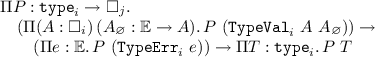
subject to the following definitional equations:

The ${\Omega }$ term describes what it means for a type to fail, i.e. it ascribes a meaning to sequents of the form $\Gamma \vdash M:{{\mathtt {fail}}\ e}$. In practice, it is irrelevant and can be chosen to be degenerate, e.g. ${\Omega }\mathrel {:=}{{\lambda {{\texttt {\_}}} : {\mathbb {E}}.\,{\mathtt {unit}}}}$.

In what follows, we often leave the universe indices implicit although they can be retrieved at the cost of more explicit annotations.

Before defining the exceptional translation we need to derive a term $\mathtt {El}$³ that recovers the underlying type from an inhabitant of $\mathtt {type}$ and $\mathtt {Err}$ that lifts the default function to this underlying type.

Definition 2

From the data of Definition 1, we derive the following terms.

Fig. 2.

Exceptional translation

The exceptional translation is defined in Fig. 2. As usual for syntactic translations [9], the term translation is given by $[{\cdot }]$ and the type translation, written $[\![{\cdot }]\!]$, is derived from it using the function $\mathtt {El}$. There is an additional macro ${[{\cdot }]}_{\varnothing }$, defined using ${\mathtt {Err}}_{i}$, which corresponds to the way to inhabit a given type from an exception.

Note that we will often slightly abuse the translation and use the $[{\cdot }]$ and $[\![{\cdot }]\!]$ notation as macros acting on the target theory. This is merely for readability purposes, and the corresponding uses are easily expanded to the actual term.

The following lemma makes explicit how $[\![{\cdot }]\!]$ and ${[{\cdot }]}_{\varnothing }$ behave on universes and on the dependent function space.

Lemma 3

(Unfoldings). The following definitional equations hold:

• ${[\![{\square }_{i}]\!]}\mathrel {\equiv }{{{\mathtt {type}}_{i}}}$

• ${[\![\Pi x : A.\,B]\!]}\mathrel {\equiv }{\Pi x : [\![A]\!].\,[\![B]\!]}$

• ${{[{\square }_{i}]}_{\varnothing }\ e}\mathrel {\equiv }{{{\mathtt {TypeErr}}_{i}}\ e}$

• ${{[\Pi x : A.\,B]}_{\varnothing }\ e}\mathrel {\equiv }{\lambda x : [\![A]\!].\,{[B]}_{\varnothing }\ e}$

Proof

By unfolding and straightforward reductions.

The soundness of the translation follows from the following properties, which are fundamental but straightforward to prove.

Theorem 4

(Soundness). The following properties hold.

• ${[M\lbrace {{x\mathrel {:=}N}}\rbrace ]}\mathrel {\equiv }{[M]\lbrace {{x\mathrel {:=}[N]}}\rbrace }$ (substitution lemma).

• If $M\mathrel {\equiv }N$ then $[M]\mathrel {\equiv }[N]$ (conversion lemma).

• If $\Gamma \vdash M:A$ then $[\![\Gamma ]\!]\vdash [M]:[\![A]\!]$ (typing soundness).

• If $\Gamma \vdash A:{\square }$ then $[\![\Gamma ]\!]\vdash {{[A]}_{\varnothing }}:{{\mathbb {E}}\rightarrow [\![A]\!]}$ (exception soundness).

Proof

The first property is by routine induction on M, the second is direct by induction on the conversion derivation. The third is by induction on the typing derivation, the most important rule being ${\square }_{i}$ : ${\square }_{j}$, which holds because ${[{\square }_{i}]}\mathrel {\equiv }{{\mathtt {TypeVal}}\ {{\mathtt {type}}_{i}}\ {{\mathtt {TypeErr}}_{i}}}$ has type ${\mathtt {type}}_{j}$ which is convertible to $[\![{\square }_{j}]\!]$ by Lemma 3. The last property is a direct application of typing soundness and unfolding of Lemma 3 for universes.

We call ${\mathcal {T}}_{\mathbb {E}}$ the theory arising from this interpretation, which is formally defined in a way similar to standard categorical constructions over dependent type theory. Terms and contexts of ${\mathcal {T}}_{\mathbb {E}}$ are simply terms and contexts of $\mathcal {T}$. A context ${\Gamma }$ is valid is ${\mathcal {T}}_{\mathbb {E}}$ whenever its translation $[\![{\Gamma }]\!]$ is valid in $\mathcal {T}$. Two terms M and N are convertible in ${\mathcal {T}}_{\mathbb {E}}$ whenever their translations [M] and [N] are convertible in $\mathcal {T}$. Finally, $\Gamma \mathrel {{\vdash }_{{\mathcal {T}}_{\mathbb {E}}}}M:A$ whenever $[\![\Gamma ]\!]\mathrel {{\vdash }_{\mathcal {T}}}[M]:[\![A]\!]$.

That is, it is possible to extend ${\mathcal {T}}_{\mathbb {E}}$ with a new constant $\mathtt {c}$ of a given type A by providing an inhabitant ${\mathtt {c}}_{\mathbb {E}}$ of the translated type $[\![A]\!]$. Then the translation is extended with ${[\mathtt {c}]}\mathrel {:=}{{\mathtt {c}}_{\mathbb {E}}}$. The potential computational rules satisfied by this new constant are directly given by the computational rules satisfied by its translation. In some sense, the new constant $\mathtt {c}$ is just syntactic sugar for ${\mathtt {c}}_{\mathbb {E}}$. Using ${\mathcal {T}}_{\mathbb {E}}$, Theorem 4 can be rephrased in the following way.

Theorem 5

If $\mathcal {T}$ interprets ${\mathrm {CC}}_{\omega }$ then so does ${\mathcal {T}}_{\mathbb {E}}$, that is, the exceptional translation is a syntactic model of ${\mathrm {CC}}_{\omega }$.

2.2 Exceptional Inductive Types

The fact that the only effect we consider is raising exceptions does not really affect the negative fragment when compared to our previous work [2], but it sure shines when it comes to interpreting inductive datatypes. Indeed, as explained in the introduction, the weaning translation only interprets a subset of $\mathrm {CIC}$, restricting dependent elimination to linear predicates. Furthermore, it also requires a few syntactic properties of the underlying monad ensuring that positivity criteria are preserved through the translation, which can be sometimes hard to obtain.

The exceptional translation diverges from the weaning translation precisely on inductives types. It allows a more compact translation of the latter, while at the same time providing a complete interpretation of $\mathrm {CIC}$, that is, including full dependent elimination.

From now on, we assume that the target theory is a predicative restriction of $\mathrm {CIC}$, i.e. that we can construct in it new inductive datatypes as we do in e.g. Coq [10], but without considering an impredicative universe. That is, all the inductive types we consider in this section live in $\square$. As a matter of fact, we slightly abuse the usual nomenclature and simply call $\mathrm {CIC}$ this predicative fragment in the remainder of the paper. We refrain from describing the generic typing rules that extend ${\mathrm {CC}}_{\omega }$ into $\mathrm {CIC}$, as they are fairly standard and would take up too much space. See for instance Werner’s thesis for a comprehensive presentation [11].

Fig. 3.

Inductive type translation

Type and Constructor Translation. As explained before, the intuitive interpretation of a type through the exceptional translation is a pair of a type and a default function from exceptions into that type. In particular, when translating some inductive type $\mathcal {I}$, we must come up with a type $[\![\mathcal {I}]\!]$ together with a default function ${\mathbb {E}}\rightarrow [\![{\mathcal {I}}]\!]$. As soon as $\mathbb {E}$ is inhabited, that means that we need $[\![{\mathcal {I}}]\!]$ to be inhabited, preferably in a canonical way. The solution is simple: just as for types where we freely added the exceptional case by means of the $\mathtt {TypeErr}$ constructor, we freely add exceptions to every inductive type.

In practice, there is an elegant and simple way to do this. It just consists in translating constructors pointwise, while adding a new dedicated constructor standing for the exceptional case. We now turn to the formal construction.

Definition 6

Let $\mathcal {I}$ be an inductive datatype with

• parameters $p_1 : P_1, {\ldots }, p_n : P_n$;

• indices $i_1 : I_1, {\ldots }, i_m : I_m$;

• constructors

  

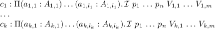
We define the exceptional translation of $\mathcal {I}$ and its constructors in Fig. 3, where ${\mathcal {I}}^{\bullet }$ is the inductive type defined by

• parameters $p_1 : {[\![{P}_{{{1}}}]\!]}, {\ldots }, p_n : {[\![{P}_{{{n}}}]\!]}$;

• indices $i_1 : {[\![{I}_{{{1}}}]\!]}, {\ldots }, i_m : {[\![{I}_{{{m}}}]\!]}$;

• constructors

  

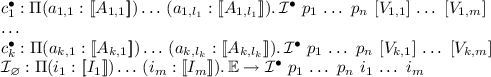
where in the recursive calls in the various A, we locally set

$$\begin{aligned} {{[\![{\mathcal {I}}\ {M}_{{{1}}}\ {{\ldots }}\ {M}_{{{n}}}\ {N}_{{{1}}}\ {{\ldots }}\ {N}_{{{m}}}]\!]}}\mathrel {:=}{{{{\mathcal {I}}^{\bullet }}\ [{M}_{{{1}}}]\ {{\ldots }}\ [{M}_{{{n}}}]\ [{N}_{{{1}}}]\ {{\ldots }}\ [{N}_{{{m}}}].}} \end{aligned}$$

Example 7

We give a few representative examples of the inductive translation in Fig. 4 in a Coq-like syntax. They were chosen because they are simple instances of inductive types featuring parameters, indices and recursion in an orthogonal way. For convenience, we write ${\Sigma }\ A\ (\lambda x : A.\,B)$ as $\Sigma x:A.\,B$.

Fig. 4.

Examples of translations of inductive types

Remark 8

The fact the we locally override the translation for recursive calls on the $[\![\cdot ]\!]$ translation of the type being defined means that we cannot handle cases where the translation of the type of a constructor actually contains an instance of $[\mathcal {I}]$. Because of the syntactic positivity criterion, the only possibility for such a situation to occur in $\mathrm {CIC}$ is in the so-called nested inductive definitions. However, nested inductive types are essentially a programming convenience, as most nested types can be rewritten in an isomorphic way that is not nested.

Lemma 9

If $\mathcal {I}$ is given as in Definition 6, we have for any terms $\vec {M}$, $\vec {N}$

$$\begin{aligned} {[\![{\mathcal {I}}\ {M}_{{{1}}}\ {{\ldots }}\ {M}_{{{n}}}\ {N}_{{{1}}}\ {{\ldots }}\ {N}_{{{m}}}]\!]}\mathrel {\equiv }{{{\mathcal {I}}^{\bullet }}\ [{M}_{{{1}}}]\ {{\ldots }}\ [{M}_{{{n}}}]\ [{N}_{{{1}}}]\ {{\ldots }}\ [{N}_{{{m}}}].} \end{aligned}$$

This justifies a posteriori the simplified local definition we used in the recursive calls of the translation of the constructors.

Theorem 10

For any inductive type $\mathcal {I}$ not using nested inductive types, the translation from Definition 6 is well-typed and satisfies the positivity criterion.

Proof

Preservation of typing is a consequence of Theorem 4. The restriction on nested types, which is slightly stronger than the usual positivity criterion of $\mathrm {CIC}$, is due to the fact that ${\mathcal {I}}_{\varnothing }$ is not available in the recursive calls and thus cannot be used to build a term of type $\mathtt {type}$ via the $\mathtt {TypeVal}$ constructor.

Preservation of the positivity criterion is straightforward, as the shape of every constructor $c_k$ is preserved, and furthermore by Lemma 3 the structure of every argument type is preserved by $[\![\cdot ]\!]$ as well. The only additional constructor ${\mathcal {I}}_{\varnothing }$ does not mention the recursive type and is thus automatically positive.

Corollary 11

Type soundness holds for the translation of inductive types and their constructors.

Pattern-Matching Translation. We now turn to the translation of the elimination of inductive terms, that is, pattern matching. Once again, its definition originates from the fact that we are working with call-by-name exceptions. It is well-known that in call-by-name, pattern matching implements a delimited form of call-by-value, by forcing its scrutinee before proceeding, at least up to the head constructor. Therefore, as soon as the matched term (re-)raises an exception, the whole pattern-matching reraises the same exception. A little care has to be taken in order to accomodate for the fact that the return type of the pattern-matching depends on the scrutinee, in particular when it is the default constructor of the inductive type.

In what follows, we use the ${i}_{{{1}}}\ {{\ldots }}\ {i}_{{{n}}}$ notation for clarity, but compact it to $\vec {i}$ for space reasons, when appropriate.

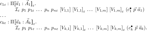
Definition 12

Assume an inductive $\mathcal {I}$ as given in Definition 6. Let Q be the well-typed pattern-matching defined as

where

then we pose [Q] to be the following pattern-matching.

Lemma 13

With notations and typing assumptions from Definition 12, we have

$$\begin{aligned} {[\![{\Gamma }]\!]}\vdash {[Q]}:{[\![R]\!]\lbrace {{{\vec {i}}\mathrel {:=}{\vec {{[Y]}}}}},{{x\mathrel {:=}[M]}}\rbrace .} \end{aligned}$$

Proof

Mostly a consequence of Theorem 4 applied to all of the premises of the pattern-matching rule. The only thing we have to check specifically is that the branch for the default constructor ${\mathcal {I}}_{\varnothing }$ is well-typed as

$$\begin{aligned} {[\![{\Gamma }]\!]}, \vec {i} : {{\vec {I}}\lbrace {{{\vec {p}}\mathrel {:=}{\vec {X}}}}\rbrace }, e : \mathbb {E}\vdash {{[R]}_{\varnothing }\lbrace {{x\mathrel {:=}{{\mathcal {I}}_{\varnothing }}\ {\vec {X}}\ {\vec {i}}\ e}}\rbrace \ e}:{[\![R]\!]\lbrace {{x\mathrel {:=}{{\mathcal {I}}_{\varnothing }}\ {\vec {X}}\ {\vec {i}}\ e}}\rbrace } \end{aligned}$$

which is also due to Theorem 4 applied to R.

Lemma 14

The translation preserves ${\iota }$-rules.

Proof

Immediate, as the translation preserves the structure of the patterns.

The translation is also applicable to fixpoints, but for the sake of readability we do not want to fully spell it out, although it is simply defined by congruence (commutation with the syntax). As such, it trivially preserves typing and reduction rules. Note that the Coq plugin presented in Sect. 6 features a complete translation of inductive types, pattern-matching and fixpoints. So the interested reader may experiment with the plugin to see how fixpoints are translated.

Therefore, by summarizing all of the previous properties, we have the following result.

Theorem 15

If $\mathcal {T}$ interprets $\mathrm {CIC}$, then so does ${\mathcal {T}}_{\mathbb {E}}$, and thus the exceptional translation is a syntactic model of $\mathrm {CIC}$.

2.3 Flirting with Inconsistency

It is now time to point at the elephant in the room. The exceptional translation has a lot of nice properties, but it has one grave defect.

Theorem 16

If $\mathbb {E}$ is inhabited, then ${\mathcal {T}}_{\mathbb {E}}$ is logically inconsistent.

Proof

The empty type is translated as

which is inhabited as soon as $\mathbb {E}$ is.

Note that when $\mathbb {E}$ is empty, the situation is hardly better, as the translation is essentially the identity. However, when $\mathcal {T}$ satisfies canonicity, the situation is not totally desperate as ${\mathcal {T}}_{\mathbb {E}}$ enjoys the following weaker canonicity lemma.

Lemma 17

(Exceptional Canonicity). Let $\mathcal {I}$ be an inductive type with constructors ${c}_{1}$, ..., ${c}_{n}$ and assume that $\mathcal {T}$ satisfies canonicity. The translation of any closed term $\mathrel {{\vdash }_{{\mathcal {T}}_{\mathbb {E}}}}M:\mathcal {I}$ evaluates either to a constructor of the form ${{c}_{i}^{\bullet }}\ {N}_{{{1}}}\ {{\ldots }}\ {{N}_{l_i}}$ or to the default constructor ${{\mathcal {I}}_{\varnothing }}\ e$ for some $e:\mathbb {E}$.

Proof

Direct application of Theorem 4 and canonicity of $\mathcal {T}$.

A direct consequence of Lemma 17 is that any proof of the empty type is an exception. As we will see in Sect. 4.1, for some types it is also possible to dynamically check whether a term of this type is a correct proof, in the sense that it does not raise an uncaught exception. This means that while ${\mathcal {T}}_{\mathbb {E}}$ is logically unsound, it is computationally relevant and can still be used as a dependently-typed programming language with exceptions, a shift into a realm where we would have called the weaker canonicity Lemma 17 a progress lemma.

This is not the end of the story, though. Recall that ${\mathcal {T}}_{\mathbb {E}}$ only exists through its embedding $[\cdot ]$ into $\mathcal {T}$. In particular, if $\mathcal {T}$ is consistent, this means that one can reason about terms of ${\mathcal {T}}_{\mathbb {E}}$ directly in $\mathcal {T}$. For instance, it is possible to prove in $\mathcal {T}$ that assuming some properties about its input, a function in ${\mathcal {T}}_{\mathbb {E}}$ never raises an exception. Hence not only do we have an effectul programming language, but we also have a sound logical framework allowing to transparently prove safety properties about impure programs.

It is actually even better than that. We will show in Sect. 3 that safety properties can be derived automatically for pure programs, allowing to recover a consistent type theory as long as $\mathcal {T}$ is consistent itself.

2.4 Living in an Exceptional World

We describe here what ${\mathcal {T}}_{\mathbb {E}}$ feels like in direct style. The exceptional theory feature a new type $\mathbf {E}$ which reifies the underlying type $\mathbb {E}$ of exceptions in ${\mathcal {T}}_{\mathbb {E}}$. It uses the fact that for $\mathbb {E}$, the default function (here of type ${\mathbb {E}}\rightarrow {\mathbb {E}}$) can simply be defined as the identity function. Its translation is given by

$$\begin{aligned} {[\mathbf {E}]:{[\![\square ]\!]}}\mathrel {:=}{{{\mathtt {TypeVal}}\ {\mathbb {E}}\ (\lambda e : {\mathbb {E}}.\,e).}} \end{aligned}$$

Then, it is possible to define in ${\mathcal {T}}_{\mathbb {E}}$ a function $\mathtt {raise}$ : $\Pi A : \square .\,{\mathbf {E}}\rightarrow A$ that raises the provided exception at any type as

$$\begin{aligned} {[\mathtt {raise}]}\mathrel {:=}{{\lambda {({A}: {\mathtt {type}})}\,{({e}: {\mathbb {E}})}.\,{\mathtt {Err}}\ A\ e.}} \end{aligned}$$

As we have already mentioned, the reader should be aware that the exceptions arising from this translation are call-by-name. This means that they do not behave like their usual call-by-value counterpart. In particular, we have in ${\mathcal {T}}_{\mathbb {E}}$

$$\begin{aligned} {{\mathtt {raise}}\ (\Pi x : A.\,B)\ e}\mathrel {\equiv }{\lambda x : A.\,{\mathtt {raise}}\ B\ e} \end{aligned}$$

which means that exceptions cannot be caught on ${\Pi }$-types. We can catch them on universes and inductive types though, because in those cases they are freely added through an extra constructor which one can pattern-match on. For instance, there exists in ${\mathcal {T}}_{\mathbb {E}}$ a term

defined by

satisfying the expected reduction rules on all three cases.

In Sect. 6, we illustrate the use of the exceptional theory using the Coq plugin to define a simple cast framework as in [12].

Fig. 5.

Parametricity over exceptional translation

3 Kreisel Meets Martin-Löf

It is well-known that Reynolds’ parametricity [13] and Kreisel’s modified realizability [4] are two instances of the broader logical relation techniques. Usually, parametricity is used to derive theorems for free, while realizability constrains programs. In a surprising turn of events, we use Bernardy’s variant of parametricity on $\mathrm {CIC}$ [5] as a realizability trick to evict undesirable behaviours of ${\mathcal {T}}_{\mathbb {E}}$. This leads to the parametric exceptional translation, which can be seen as the embodiment of Kreisel’s realizability in type theory. In this section, we first present this translation on the negative fragment, then extend it to $\mathrm {CIC}$ and finally discuss its meta-theoretical properties.

3.1 Exceptional Parametricity in a Negative World

The exceptional parametricity translation for terms of ${\mathrm {CC}}_{\omega }$ is defined in Fig. 5. Intuitively, any type A in ${\mathcal {T}}_{\mathbb {E}}$ is turned into a validity predicate ${A}_{\varepsilon }:{A\rightarrow \square }$ which encodes the fact that an inhabitant of A is not allowed to generate unhandled exceptions. For instance, a function is valid if its application to a valid term produces a valid answer. It does not say anything about the application to invalid terms though, which amounts to a garbage in, garbage out policy. The translation then states that every pure term is automatically valid.

This translation is exactly standard parametricity for type theory [5] but parametrized by the exceptional translation. This means that any occurrence of a term of the original theory used in the parametricity translation is replaced by its exceptional translation, using $[{\cdot }]$ or $[\![{\cdot }]\!]$ depending on whether it is used as a term or as a type. For instance, the translation of an application ${[M\ N]}_{\varepsilon }$ is given by ${[M]}_{\varepsilon }\ [N]\ {[N]}_{\varepsilon }$ instead of just ${[M]}_{\varepsilon }\ N\ {[N]}_{\varepsilon }$.

Lemma 18

(Substitution lemma). The translation satisfies the following conversion: ${{[M\lbrace {{x\mathrel {:=}N}}\rbrace ]}_{\varepsilon }}\mathrel {\equiv }{{[M]}_{\varepsilon }\lbrace {{x\mathrel {:=}[N]}},{{{{x}_{\varepsilon }}\mathrel {:=}{[N]}_{\varepsilon }}}\rbrace }$.

Theorem 19

(Soundness). The two following properties hold.

• If $M\mathrel {\equiv }N$ then ${{[M]}_{\varepsilon }}\mathrel {\equiv }{{[N]}_{\varepsilon }}$.

• If $\Gamma \vdash M:A$ then ${[\![\Gamma ]\!]}_{\varepsilon }\vdash {{[M]}_{\varepsilon }}:{{[\![A]\!]}_{\varepsilon }\ [M]}$.

Proof

By induction on the derivation.

We can use this result to construct another syntactic model of ${\mathrm {CC}}_{\omega }$. Contrarily to usual syntactic models where sequents are straightforwarldy translated to sequents, this model is slightly more subtle as sequents are translated to pairs of sequents instead. This is similar to the usual parametricity translation.

Definition 20

The theory ${\mathcal {T}}_{\mathbb {E}}^{p}$ is defined by the following data.

• Terms of ${\mathcal {T}}_{\mathbb {E}}^{p}$ are pairs of terms of $\mathcal {T}$.

• Contexts of ${\mathcal {T}}_{\mathbb {E}}^{p}$ are pairs of contexts of $\mathcal {T}$.

• $\mathrel {{\vdash }_{{\mathcal {T}}_{\mathbb {E}}^{p}}}\Gamma$ whenever $\mathrel {{\vdash }_{\mathcal {T}}}[\![\Gamma ]\!]$ and $\mathrel {{\vdash }_{\mathcal {T}}}{[\![\Gamma ]\!]}_{\varepsilon }$.

• $M\mathrel {{\equiv }_{{\mathcal {T}}_{\mathbb {E}}^{p}}}N$ whenever $[M]\mathrel {{\equiv }_{\mathcal {T}}}[N]$ and ${[M]}_{\varepsilon }\mathrel {{\equiv }_{\mathcal {T}}}{[N]}_{\varepsilon }$.

• $\Gamma \mathrel {{\vdash }_{{\mathcal {T}}_{\mathbb {E}}^{p}}}M:A$ whenever $[\![\Gamma ]\!]\mathrel {{\vdash }_{\mathcal {T}}}[M]:[\![A]\!]$ and ${[\![\Gamma ]\!]}_{\varepsilon }\mathrel {{\vdash }_{\mathcal {T}}}{[M]}_{\varepsilon }:{{[\![A]\!]}_{\varepsilon }\ [M]}$.

Once again, Theorem 19 can be rephrased in terms of preservation of theories and syntactic models.

Theorem 21

If $\mathcal {T}$ interprets ${\mathrm {CC}}_{\omega }$ then so does ${\mathcal {T}}_{\mathbb {E}}^{p}$. That is, the parametric exceptional translation is a syntactic model of ${\mathrm {CC}}_{\omega }$.

This construction preserves definitional ${\eta }$-expansion, as functions are mapped to (slightly more complicated) functions.

Lemma 22

If $\mathcal {T}$ satisfies definitional ${\eta }$-expansion, then so does ${\mathcal {T}}_{\mathbb {E}}^{p}$.

Proof

The first component of the translation preserves definitional ${\eta }$-expansion because functions are mapped to functions. It remains to show that

$$\begin{aligned} {{{[\lambda x : A.\,M\ x]}_{\varepsilon }}}\mathrel {:=}{{\lambda {({x}: [\![A]\!])}\,{({{{x}_{\varepsilon }}}: {[\![A]\!]}_{\varepsilon }\ x)}.\,{[M]}_{\varepsilon }\ x\ {{x}_{\varepsilon }}}}\mathrel {\equiv }{{[M]}_{\varepsilon }} \end{aligned}$$

which holds by applying ${\eta }$-expansion twice.

It is interesting to remark that Bernardy-style unary parametricity also leads to a syntactic model ${\mathcal {T}}^{p}$ that interprets ${\mathrm {CC}}_{\omega }$ (as well as $\mathrm {CIC}$), using the same kind of glueing construction. Nonetheless, this model is somewhat degenerate from the logical point of view. Namely it is a conservative extension of the target theory. Indeed, if $\Gamma \mathrel {{\vdash }_{{\mathcal {T}}^{p}}}M:A$ for some ${\Gamma }$, M and A from $\mathcal {T}$, then there we also have $\Gamma \mathrel {{\vdash }_{\mathcal {T}}}M:A$, because the first component of the model is the identity, and the original sequent can be retrieved by the first projection.

This is definitely not the case with the ${\mathcal {T}}_{\mathbb {E}}^{p}$ theory, because the first projection is not the identity. In particular, because of Theorem 16, every sequent in the first projection is inhabited, although it is not the case in $\mathcal {T}$ itself if it is consistent. This means that parametricity can actually bring additional expressivity when it applies to a theory which is not pure, as it is the case here.

Fig. 6.

Examples of parametric translation of inductive types

3.2 Exceptional Parametric Translation of $\mathrm {CIC}$

We now describe the parametricity translation of the positive fragment. The intuition is that as it stands for an exception, the default constructor is always invalid, while all other constructors are valid, assuming their arguments are.

Type and Constructor Translation

Definition 23

Let $\mathcal {I}$ be an inductive type as given in Definition 6. We define the exceptional parametricity translation ${\mathcal {I}}_{\varepsilon }$ of $\mathcal {I}$ as the inductive type defined by:

• parameters ${[\![p_1 : P_1, {\ldots }, p_n : P_n]\!]}_{\varepsilon }$;

• indices ${[\![i_1 : I_1, {\ldots }, i_m : I_m]\!]}_{\varepsilon }, x : {{\mathcal {I}}\ {p}_{{{1}}}\ {{\ldots }}\ {p}_{{{n}}}\ {i}_{{{1}}}\ {{\ldots }}\ {i}_{{{m}}}}$;

• constructors

  

and we extend the translation as

Example 24

We give the exceptional parametric inductive translation of our running examples in Fig. 6.

Note that contrarily to the negative case, the exceptional parametricity translation on inductive types is not the same thing as the composition of Bernardy’s parametricity together with the exceptional translation. Indeed, the latter would also have produced a constructor for the default case from the exceptional inductive translation, whereas our goal is precisely to rule this case out via the additional realizability-like interpretation.

It is also very different from our previous parametric weaning translation [2], which relies on internal parametricity to recover dependent elimination, enforcing by construction that no effectful term exists. Here, effectful terms may be used in the first component, but they are required after the fact to have no inconsistent behaviour. Intuitively, parametric weaning produces one pure sequent, while exceptional parametricity produces two, with the first one being potentially impure and the second one assuring the first one is harmless.

Pattern-Matching Translation

Definition 25

Let Q be the pattern-matching defined in Definition 12. We pose ${[Q]}_{\varepsilon }$ to be the pattern-matching

where $Q_x$ is the following pattern-matching

that is Q where the scrutinee has been turned into the index variable of the parametricity predicate.

Lemma 26

With notations and typing assumptions from Definition 12, we have

$$\begin{aligned} {{[\![{\Gamma }]\!]}_{\varepsilon }}\vdash {{[Q]}_{\varepsilon }}:{{[\![R\lbrace {{{\vec {i}}\mathrel {:=}{\vec {{Y}}}}},{{x\mathrel {:=}M}}\rbrace ]\!]}_{\varepsilon }\ [Q].} \end{aligned}$$

The exceptional parametricity translation can be extended to handle fixpoints as well, with a few limitations. Translating generic fixpoints uniformly is indeed an open problem in standard parametricity, and our variant faces the same issue. In practice, standard recursors can be automatically translated, and fancy fixpoints may require hand-writing the parametricity proof. We do not describe the recursor translation here though, as it is essentially the same as standard parametricity. Again, the interested reader may test the Coq plugin exposed in Sect. 6 to see how recursors are translated.

Packing everything together allows to state the following result.

Theorem 27

If $\mathcal {T}$ interprets $\mathrm {CIC}$, then so does ${\mathcal {T}}_{\mathbb {E}}^{p}$, and thus the exceptional parametricity translation is a syntactic model of $\mathrm {CIC}$.

3.3 Meta-Theoretical Properties of ${\mathcal {T}}_{\mathbb {E}}^{p}$

Being built as a syntactic model, ${\mathcal {T}}_{\mathbb {E}}^{p}$ inherits a lot of meta-theoretical properties of $\mathcal {T}$. We list a few of interest below.

Theorem 28

If $\mathcal {T}$ is consistent, then so is ${\mathcal {T}}_{\mathbb {E}}^{p}$.

Proof

Assume $\mathrel {{\vdash }_{{\mathcal {T}}_{\mathbb {E}}^{p}}}M_0:\mathtt {empty}$ for some $M_0$. Then by definition, there exists two terms M and ${M}_{\varepsilon }$ such that $\mathrel {{\vdash }_{\mathcal {T}}}M:{\mathtt {empty}}^{\bullet }$ and $\mathrel {{\vdash }_{\mathcal {T}}}{M}_{\varepsilon }:{{{\mathtt {empty}}_{\varepsilon }}\ M}$. But ${\mathtt {empty}}_{\varepsilon }$ has no constructor, and $\mathcal {T}$ is inconsistent.

More generally, the same argument holds for any inductive type.

Theorem 29

If $\mathcal {T}$ enjoys canonicity, then so does ${\mathcal {T}}_{\mathbb {E}}^{p}$.

Proof

The exceptional parametricity translation for inductive types has the same structure as the original type, so any normal form in ${\mathcal {T}}_{\mathbb {E}}^{p}$ can be mapped back to a normal form in $\mathcal {T}$.

4 Effectively Extending $\mathrm {CIC}$

The parametric exceptional translation allows to extend the logical expressivity of $\mathrm {CIC}$ in the following ways, which we develop in the remainder of this section.

We show in Sect. 4.1 that Markov’s rule is admissible in $\mathrm {CIC}$. We already sketched this result in our previous paper [2], but we come back to it in more details. More generally, we show a form of conservativity of double-negation elimination over the type-theoretic version of ${\Pi }_{2}^{0}$ formulae.

In Sect. 4.2, we exhibit a syntactic model of $\mathrm {CIC}$ which satisfies definitional ${\eta }$-expansion for functions but which negates function extensionality. As far as we know, this was not known.

Finally, in Sect. 4.3, we show that there exists a model of $\mathrm {CIC}$ which validates the independence of premises. This is a new result, that shows that $\mathrm {CIC}$ can feature traces of classical reasoning while staying computational. We use this result in Sect. 4.4 to give an alternative proof of the recent result of Coquand and Mannaa [7] that Markov’s principle is not provable in $\mathrm {CIC}$.

4.1 Markov’s Rule

We show in this section that $\mathrm {CIC}$ is closed under a generalized Markov’s rule. The technique used here is no more than a dependently-typed variant of Friedman’s trick [14]. Indeed, Friedman’s A-translation amounts to add exceptions to intuitionistic logic, which is precisely what ${\mathcal {T}}_{\mathbb {E}}$ does for $\mathrm {CIC}$.

Definition 30

An inductive type in $\mathrm {CIC}$ is said to be first-order if all the types of the arguments of its constructors, in its parameters and in its indices are recursively first-order.

Example 31

The $\mathtt {empty}$, $\mathtt {unit}$ and $\mathbb {N}$ types are first-order. If P and Q are first-order then so is $\Sigma p:P.\,Q$, $P + Q$ and $\mathtt {eq}\ P\ {p}_{{{0}}}\ {p}_{{{1}}}$. Consequently, the $\mathrm {CIC}$ equivalent of ${\Sigma }_{1}^{0}$ formulae are in particular first-order.

First-order types enjoy uncommon properties, like the fact that they can be injected into effectful terms and purified away. This is then used to prove the generalized Markov’s Rule.

Lemma 32

For every first-order type $\vec {p}:\vec {P}\vdash Q:{\square }$ where all $\vec {P}$ are first-order, there are retractions ${\iota }_{\vec {P}}$, ${\iota }_{Q}$ and ${\theta }_{\vec {P}}$, ${\theta }_{Q}$ s.t.:

Proof

The ${\iota }$ terms exist because effectful inductive types are a semantical superset of their pure equivalent, and the ${\theta }$ terms are implemented by recursively forcing the corresponding impure inductive term. One relies on decidability of equality of first-order type to fix the indices.

Theorem 33

(Generalized Markov’s Rule). For any first-order type P and first-order predicate Q over P, if $\ \mathrel {{\vdash }_{\mathrm {CIC}}}{\Pi p : P.\,{\lnot \lnot }\ (Q\ p)}$ then $\ \mathrel {{\vdash }_{\mathrm {CIC}}}{\Pi p : P.\,Q\ p}$.

Proof

Let $\vdash M:{\Pi p : P.\,{\lnot \lnot }\ (Q\ p)}$. By taking ${\mathbb {E}}\mathrel {:=}{{Q\ p}}$ and apply the soundness theorem, one gets a proof

$$\begin{aligned} p : P\vdash {[M]}:{\Pi {\hat{p}} : [\![P]\!].\,([\![Q\ {\hat{p}}]\!]\rightarrow {{\mathtt {empty}}^{\bullet }})\rightarrow {{\mathtt {empty}}^{\bullet }}.} \end{aligned}$$

But ${\mathtt {empty}}^{\bullet }\cong \mathbb {E}\equiv {Q\ p}$, so we can derive from [M] a term ${M}^{\sharp }$ s.t.

$$\begin{aligned} p : P\vdash {M}^{\sharp }:{\Pi {\hat{p}} : [\![P]\!].\,([\![Q\ {\hat{p}}]\!]\rightarrow Q\ p + Q\ p)\rightarrow Q\ p.} \end{aligned}$$

The proofterm we were looking for is thus no more than $\lambda p : P.\,{{M}^{\sharp }}\ ({{\iota }_{P}}\ p)\ {{\theta }_{Q}}$.

4.2 Function Intensionality with ${\eta }$-expansion

In a previous paper [9], we already showed that there existed a syntactic model of $\mathrm {CIC}$ that allowed to internally disprove function extensionality. Yet, this model was clearly not preserving definitional ${\eta }$-expansion on functions, as it was adding additional structure to abstraction and application (namely a boolean). Thanks to our new model, we can now demonstrate that counterintuitively, it is possible to have a consistent type theory that enjoys definitional ${\eta }$-expansion while negating internally function extensionality. In this section we suppose that ${\mathbb {E}}\mathrel {:=}{\mathtt {unit}}$, although any inhabited type of exceptions would work.

By Lemma 22, we know that the parametric exceptional translation preserves definitional ${\eta }$-expansion. It is thus sufficient to find two functions that are extensionally equal but intensionally distinct in the model. Let us consider to this end the ${\mathtt {unit}}\rightarrow {\mathtt {unit}}$ functions

Theorem 34

The following sequents are derivable:

Proof

The main difference between the two functions is that ${\mathtt {id}}_{{\bot }}$ preserves exceptions while ${\mathtt {id}}_{\top }$ does not, which we exploit.

The first sequent is provable in $\mathrm {CIC}$ by dependent elimination and thus is derivable in ${\mathcal {T}}_{\mathbb {E}}^{p}$ by applying the soundness theorem.

To prove the first component of the second sequent, we exhibit a property that discriminates $[{{\mathtt {id}}_{{\bot }}}]$ and $[{{\mathtt {id}}_{\top }}]$, which is, as explained, their evaluation on the term ${{\mathtt {unit}}_{\varnothing }}\ {\mathtt {tt}}$. Showing then that this proof is parametric is equivalent to showing $\Pi {({p}: [\![{{\mathtt {id}}_{{\bot }}} = {{\mathtt {id}}_{\top }}]\!])}\,{({{{p}_{\varepsilon }}}: {[\![{{\mathtt {id}}_{{\bot }}} = {{\mathtt {id}}_{\top }}]\!]}_{\varepsilon }\ p)}.\,{\mathtt {empty}}$. But ${p}_{\varepsilon }$ actually implies $[{{\mathtt {id}}_{{\bot }}}] = [{{\mathtt {id}}_{\top }}]$, which we just showed was absurd.

4.3 Independence of Premise

Independence of premise (IP) is a semi-classical principle from first-order logic whose $\mathrm {CIC}$ equivalent can be stated as follows.

$$\begin{aligned} {\Pi {({A}: \square )}\,{({B}: {\mathbb {N}}\rightarrow \square )}.\,(\lnot A\rightarrow \Sigma n:{\mathbb {N}}.\,B\ n)\rightarrow \Sigma n:{\mathbb {N}}.\,\lnot A\rightarrow B\ n}\quad \text{(IP) } \end{aligned}$$

Although not derivable in intuitionistic logic, it is an admissible rule of $\mathbf {HA}$. The standard proof of this property is to go through Kreisel’s modified realizability interpretation of $\mathbf {HA}$ [4]. In a nutshell, the interpretation goes as follows: by induction over a formula A, define a simple type $\tau (A)$ of realizers of A together with a realizability predicate $\cdot \Vdash A$ over $\tau (A)$. Then show that whenever $\ \mathrel {{\vdash }_{\mathbf {HA}}}A$, there exists some simply-typed term $t : \tau (A)$ s.t. $t\Vdash A$. As the interpretation also implies that there is no t s.t. $t\Vdash {\bot }$, this gives a sound model of $\mathbf {HA}$, which contains more than the latter. Most notably, there is for instance a term $\mathtt {ip}$ s.t.

$$\begin{aligned} \mathtt {ip}\Vdash {(\lnot A\rightarrow {\exists n.\,B})\rightarrow {\exists n.\,{\lnot A\rightarrow B}}} \end{aligned}$$

for any A, B. Intriguingly, the computational content of $\mathtt {ip}$ did not seem to receive a fair treatment in the literature. To the best of our knowledge, it has never been explicitly stated that IP was realizable because of the following “bug” of Kreisel’s modified realizability.

Lemma 35

(Kreisel’s bug). For every formula A, $\tau (A)$ is inhabited. In particular, ${\tau ({\bot })}\mathrel {:=}{\mathtt {unit}}$.

We show that this is actually not a bug, but a hidden feature of Kreisel’s modified realizability, which secretly allows to encode exceptions in the realizers. To this end, we implement IP in ${\mathcal {T}}_{\mathbb {E}}^{p}$ by relying internally on paraproofs, i.e. terms raising exceptions, while ensuring these exceptions never escape outside of the locally unsafe boundary. The resulting ${\mathcal {T}}_{\mathbb {E}}^{p}$ term has essentially the same computational content as its Kreisel’s realizability counterpart. In this section we suppose that ${\mathbb {E}}\mathrel {:=}{\mathtt {unit}}$, although assuming $\mathbb {E}$ to be inhabited is sufficient.

To ease the understanding of the definition, we rely on effectful combinators that can be defined in ${\mathcal {T}}_{\mathbb {E}}$.

Definition 36

We define in ${\mathcal {T}}_{\mathbb {E}}$ the following terms.

It is worth insisting that these combinators are not necessarily parametric. While it can be shown that ${\mathtt {is}}_{\Sigma }$ and ${\mathtt {is}}_{\mathbb {N}}$ actually are, $\mathtt {fail}$ is luckily not. The ${\mathtt {is}}_{\Sigma }$ and ${\mathtt {is}}_{\mathbb {N}}$ functions are used in order to check that a value is actually pure and does not contain exceptions.

Definition 37

We define $\mathtt {ip}$ in ${\mathcal {T}}_{\mathbb {E}}$ in direct style below, using the available combinators from Definition 36 and a bit of syntactic sugar.

The intuition behind this term is the following. Given $f:{\lnot A\rightarrow \Sigma n:{\mathbb {N}}.\,B\ n}$, we apply it to a dummy function which fails whenever it is used. Owing to the semantics of negation, we know in the parametricity layer that the only way for this application to return an exception is that f actually contained a proof of A and applied $\mathtt {fail}$ to it. Therefore, given a true proof of $\lnot A$, we are in an inconsistent setting and thus we are able to do whatever pleases us. The issue is that we do not have access to such a proof yet, and we do have to provide a valid integer now. Therefore, we check whether f actually provided us with a valid pair containing a valid integer. If so, this is our answer, otherwise we stuff a dummy integer value and we postpone the contradiction.

This is essentially the same realizer as the one from Kreisel’s modified realizability, except that we have a fancy type system for realizers. In particular, because we have dependent types, integers also exist in the logical layer, so that they need to be checked for exceptions as well. The only thing that remains to be proved is that $\mathtt {ip}$ also lives in ${\mathcal {T}}_{\mathbb {E}}^{p}$.

Theorem 38

There is a proof of $\mathrel {{\vdash }_{\mathcal {T}}}{{[\![{\mathrm {IP}}]\!]}_{\varepsilon }\ {[\mathtt {ip}]}}$.

Proof

The proof is straightforward but tedious, so we do not give the full details. The file IPc.v of the companion Coq plugin contains an explicit proof. The essential properties that make it go through are the following.

• $\ \mathrel {{\vdash }_{\mathcal {T}}}{\Pi {({n}: {{\mathbb {N}}^{\bullet }})}\,{({{p}_{{{1}}}}\,{{p}_{{{2}}}}: {{\mathbb {N}}_{\varepsilon }}\ n)}.\,{p}_{{{1}}} = {p}_{{{2}}}}$

• $\ \mathrel {{\vdash }_{\mathcal {T}}}{\Pi n : {{\mathbb {N}}^{\bullet }}.\,{{[{{\mathtt {is}}_{\mathbb {N}}}]\ n = {\mathtt {true}}^{\bullet }}\leftrightarrow {{{\mathbb {N}}_{\varepsilon }}\ n}}}$

• $\ \mathrel {{\vdash }_{\mathcal {T}}}{\Pi {({p}\,{q}: [\![\lnot A]\!])}.\,{[\![\lnot A]\!]}_{\varepsilon }\ p\rightarrow {[\![\lnot A]\!]}_{\varepsilon }\ q}$

Corollary 39

We have $\ \mathrel {{\vdash }_{{\mathcal {T}}_{\mathbb {E}}^{p}}}\mathrm {IP}$.

4.4 Non-provability of Markov’s Principle

From this result, one can get a very easy syntactic proof of the independence result of Markov’s principle from $\mathrm {CIC}$. Markov’s principle is usually stated as

$$\begin{aligned} {\Pi P : {\mathbb {N}}\rightarrow {\mathtt {bool}}.\,{\lnot \lnot }\ (\Sigma n:{\mathbb {N}}.\,P\ n = \mathtt {true})\rightarrow \Sigma n:{\mathbb {N}}.\,P\ n = \mathtt {true}}\quad \text{(MP) } \end{aligned}$$

An independence result was recently proved by Coquand and Mannaa by a semantic argument [7]. We leverage instead a property from realizability [15] that has been applied to type theory the other way around by Herbelin [16].

Lemma 40

If $\mathcal {S}$ is a computable theory containing $\mathrm {CIC}$ and enjoying canonicity, then one cannot have both $\mathrel {{\vdash }_{\mathcal {S}}}\mathrm {IP}$ and $\mathrel {{\vdash }_{\mathcal {S}}}\mathrm {MP}$.

Proof

By applying $\mathrm {IP}$ to $\mathrm {MP}$, one easily obtains that

$$\begin{aligned} \ \mathrel {{\vdash }_{\mathcal {S}}}{\Pi P : {\mathbb {N}}\rightarrow {\mathtt {bool}}.\,\Sigma n:{\mathbb {N}}.\,\Pi m : {\mathbb {N}}.\,P\ m = \mathtt {true}\rightarrow P\ n = \mathtt {true}.} \end{aligned}$$

Thus, for every closed $P:{{\mathbb {N}}\rightarrow {\mathtt {bool}}}$, by canonicity there exists a closed $n_P:\mathbb {N}$ s.t. $\ \mathrel {{\vdash }_{\mathcal {S}}}{\Pi m : {\mathbb {N}}.\,P\ m = \mathtt {true}\rightarrow P\ {n}_{{{P}}} = \mathtt {true}}$. But then one can decide whether P holds for some n by just computing $P\ {n}_{{{P}}}$, so that we effectively obtained an oracle deciding the halting problem (which is expressible in $\mathrm {CIC}$).

Corollary 41

We have $\mathrel {{\not \vdash }_{{\mathrm {CIC}}_{\mathbb {E}}^{p}}}\mathrm {MP}$ and thus also $\mathrel {{\not \vdash }_{\mathrm {CIC}}}\mathrm {MP}$.

5 Possible Extensions

5.1 Negative Records

Interestingly, the fact that the translation introduces effects has unintented consequences on a few properties of type theory that are often taken for granted. Namely, because type theory is pure, there is a widespread confusion amongst type theorists between positive tuples and negative records.

• Positive tuples are defined as a one-constructor inductive type, introduced by this constructor and eliminated by pattern-matching. They do not (and in general cannot, for typing reasons) satisfy definitional ${\eta }$-laws, also known as surjective pairing.

• Negative records are defined as a record type, introduced by primitive packing and eliminated by projections. They naturally obey definitional ${\eta }$-laws.

In the remainder of this section, we will focus on the specific case of pairs, but the same arguments are generalizable to arbitrary records. Positive pairs $\Sigma x:A.\,B$ are defined by the inductive type from Fig. 4. Negative pairs are defined as a primitive structure in Fig. 7. We use the ampersand notation as a reference to linear logic.

Fig. 7.

Negative pairs

Fig. 8.

Exceptional translation of negative pairs

In $\mathrm {CIC}$, it is possible to show that negative and positive pairs are propositionally isomorphic, because positive pairs enjoy dependent elimination. Nonetheless, it is a well-known fact in the programming folklore that in a call-by-name language with effects, the two are sharply distinct. For instance, in presence of exceptions, assuming $\vdash M:{\Sigma x:A.\,B}$, one does not have in general

$$\begin{aligned} M\mathrel {\equiv }{{\mathtt {ex}}\ A\ B\ ({\mathtt {fst}}\ A\ B\ M)\ ({\mathtt {snd}}\ A\ B\ M)} \end{aligned}$$

where $\mathtt {fst}$ and $\mathtt {snd}$ are defined by pattern-matching. Indeed, if M is itself an exception, the two sides can be discriminated by a pattern-matching. Matching on the left-hand side results in immediate reraising of the exception, while matching on the right-hand side succeeds as long as the arguments of the constructor are not forced. Forcefully equating those two terms would then result in a trivial equational theory.

Such a phenomenon is at work in the exceptional translation. It is actually possible to interpret negative pairs through the translation, but in a way that significantly differs from the translation of positive pairs. In this section, we assume that $\mathcal {T}$ contains negative pairs.

Definition 42

The translation of negative pairs is given in Fig. 8.

It is straightforward to check that the definitions of Fig. 8 preserve the conversion and typing rules from Fig. 7. The same translation can be extended to any record. We thus have the following theorem.

Theorem 43

If $\mathcal {T}$ has negative records, then so has ${\mathcal {T}}_{\mathbb {E}}$.

It is enlightening to look at the difference between negative and positive pairs through the translation, because now we have effects that allow to separate them clearly. Indeed, compare

Clearly, if $\mathbb {E}$ is inhabited, then the two types do not even have the same cardinal, assuming A and B are finite. Furthermore, their default inhabitant is not the same at all. It is defined pointwise for negative pairs, while it is a special constructor for positive ones. Finally, there is obviously not any chance that $[\![\Sigma x:A.\,B]\!]$ satisfies definitional surjective pairing in vanilla $\mathrm {CIC}$, as it has two constructors. The trick is that the two types are externally distinguishable, but are not internally so, because ${\mathcal {T}}_{\mathbb {E}}$ is a model of $\mathrm {CIC}$+& and thus proves that they are propositionally isomorphic.

It is possible to equip negative pairs with a parametricity relation defined as a primitive record which is the pointwise parametricity relation of each field, which naturally preserve typing and conversion rules.

Theorem 44

If $\mathcal {T}$ has negative records, then so has ${\mathcal {T}}_{\mathbb {E}}^{p}$.

5.2 Impredicative Universe

All the systems we have considered so far are predicative. It is nonetheless possible to implement an impredicative universe $*$ in ${\mathcal {T}}_{\mathbb {E}}$ if $\mathcal {T}$ features one.

Intuitively, it is sufficient to ask for an inductive type $\mathtt {prop}$ living in ${\square }_{i}$ for all i, which is defined just as $\mathtt {type}$, except that its constructor $\mathtt {PropVal}$ corresponding to $\mathtt {TypeVal}$ contains elements of $*$ rather than $\square$. Then one can similarly define ${\mathtt {El}}_{*}$ and ${\mathtt {Err}}_{*}$ acting on $\mathtt {prop}$ rather than $\mathtt {type}$. One then slightly tweaks the $[\![{\cdot }]\!]$ macro from Fig. 2 by defining it instead as

and similarly for type constructors. With this modified translation, one obtains a soundness theorem for ${\mathrm {CC}}_{\omega }$.

Theorem 45

The exceptional translation is a syntactic model of ${\mathrm {CC}}_{\omega }+*$.

Likewise, the inductive translation is amenable to interpret an impredicative universe, with one major restriction though.

Theorem 46

The exceptional translation is a syntactic model of $\mathrm {CIC}+*$ without the singleton elimination rule.

Indeed, the addition of the default constructor disrupts the singleton elimination criterion for all inductive types. Actually, this criterion is very fragile, and even if ${\mathcal {T}}_{\mathbb {E}}$ satisfied it, Keller and Lasson showed that the parametricity translation could not interpret inductive types in $*$ for similar reasons [17], and ${\mathcal {T}}_{\mathbb {E}}^{p}$ would face the same issue.

6 The Exceptional Translation in Practice

6.1 Implementation as a Coq Plugin

The (parametric) exceptional translation is a translation of $\mathrm {CIC}$ into itself, which means that we can directly implement it as a Coq plugin. This way, we can use the translation to extend safely Coq with new logical principles, so that typechecking remains decidable.

Such a Coq plugin is simply a program that, given a Coq proof term M, produces the translations [M] and ${[M]}_{\varepsilon }$ as Coq terms. For instance, the translations of type , given in Figs. 4 and 6, are obtained by typing the following commands, which define each one new inductive type in Coq.

The first command produces only $[{\mathtt {list}}]$, while the second produces ${[{\mathtt {list}}]}_{\varepsilon }$. But the main interest of the translation is that we can exhibit new constructors. For instance, the operation described in Sect. 2.4 is defined as

6.2 Usecase: A Cast Framework

We can use the ability to raise exception to define partial function in the exceptional layer. For instance, given a decidable property (described by the type class below), it is then possible to define a cast function from to returning the converted value if the property is satisfied and raising an exception otherwise (using an inhabitant of ).

Using this cast mechanism, it is easy to define a function from lists to pairs by first converting the list into a list size two, using the impure function and then recovering a pair from a list of size two using a pure function.

In the exceptional layer, it is possible to prove the following property

in at least two way. One can perfectly prove it by simply raising an exception at top level, or by reflexivity—using the fact that actually reduces to .

However, there is a way to distinguish between those two proofs in the target theory, here Coq, by stating the following lemma which can only proven for the proof not raising an exception.

where underscores represent arguments inferred by Coq.

7 Related Work

Adding Dependency to an Effectful Language. There are numerous works on adding dependent types in mainstream effectful programming languages. They all mostly focused on how to appropriately restrict effectful terms from appearing in types. Indeed, if types only depend on pure terms, the problem of having two different evaluations of the effect of the term (at the level of types and at the level of terms) disappear. This is the case for instance for Dependent ML of Xi and Pfenning [18], or more recently for Casinghino et al. [19] on how to combine proofs and programs when programs can be non-terminating. The ${F}^{\star }$ programming language of Swamy et al. [20] uses a notion of primitive effects including state, exceptions, divergence and IO. Each effect is described through a monadic predicate transformer semantics which allows to have a pure core dependent language to reason on those effects. On a more foundational side, there are two recent and overlapping lines of work on the description of a dependent call-by-push-value (CBPV) by Ahman et al. [21] and Vákár [22]. Those works also use a purity restriction for dependency, but using the CBPV language, deals with any effect described in monadic style. On another line of work, Brady advocates for the use of algebraic effects as an elegant way to allow combing effects more smoothly than with a monadic approach and gives an implementation in Idris [23].

Adding Effects to a Dependently-Typed Language. Nanevski et al. [24] have developed Hoare type theory (HTT) to extend Coq with monadic style effects. To this end, they provide an axiomatic extension of Coq with a monad in which to encapsulate imperative code. Important tools have been developed on HTT, most notably the Ynot project [25]. Apart from being axiomatic, their monadic approach does not allow to mix effectful programs and dependency but is rather made for proving inside Coq properties on simply typed imperative programs.

Internal Translation of Type Theory. A non-axiomatic way to extend type theory with new features is to use internal translation, that is translation of type theory into itself as advocated by Boulier et al. [9]. The presentation of parametricity for type theory given by Bernardy and Lasson [5] can be seen as one of the first internal translation of type theory. However, this one does not add any new power to type theory as it is a conservative extension. Barthe et al. [26] have described a CPS translation for ${\mathrm {CC}}_{\omega }$ featuring call-cc, but without dealing with inductive types and relying on a form of type stratification. A variant of this translation has been extended recently by Bowman et al. [27] to dependent sums using answer-type polymorphism $\Pi {\alpha } : \square .\,(A\rightarrow {\alpha })\rightarrow {\alpha }$. A generic class of internal translations has been defined by Jaber et al. [28] using forcing, which can be seen as a type theoretic version of the presheaf construction used in categorical logic. This class of translation works on all $\mathrm {CIC}$ but for a restricted version of dependent elimination, identical to the Baclofen type theory [2]. Therefore, to the best of our knowledge, the exceptional translation is the first complete internal translation of $\mathrm {CIC}$ adding a particular notion of effect.

8 Conclusion and Future Work

In this paper, we have defined the exceptional translation, the first syntactic translation of the Calculus of Inductive Constructions into itself, adding effects and that covers full dependent elimination. This results in a new type theory, which features call-by-name exceptions with decidable type-checking and a weaker form of canonicity. We have shown that although the resulting theory is inconsistent, it is possible to reason on exceptional programs and show that some of them actually never raise an exception by relying on the target theory. This provides a sound logical framework allowing to transparently prove safety properties about impure dependently-typed programs. Then, using parametricity, we have given an additional layer at the top of the exceptional translation in order to tame exceptions and preserve consistency. This way, we have consistently extended the logical expressivity of CIC with independence of premises, Markov’s rule, and the negation of function extensionality while retaining ${\eta }$-expansion. Both translations have been implemented in a Coq plugin, which we use to formalize the examples.

One of the main directions of future work is to investigate whether other kind of effects can give rise to an internal translation of $\mathrm {CIC}$. To that end, it seems promising to look at algebraic presentation of effects. Indeed, the recent work on the non-necessity of the value restriction policy for algebraic effects and handlers of Kammar and Pretnar [29] suggests that we should be able to perform similar translations on $\mathrm {CIC}$ with full dependent elimination for other algebraic effects and handlers than exceptions.

References

Moggi, E.: Notions of computation and monads. Inf. Comput. 93(1), 55–92 (1991)
Pédrot, P., Tabareau, N.: An effectful way to eliminate addiction to dependence. In: 32nd Annual Symposium on Logic in Computer Science, LICS 2017, Reykjavik, Iceland, 20–23 June 2017, pp. 1–12 (2017)
Munch-Maccagnoni, G.: Models of a non-associative composition. In: Muscholl, A. (ed.) FoSSaCS 2014. LNCS, vol. 8412, pp. 396–410. Springer, Heidelberg (2014). https://doi.org/10.1007/978-3-642-54830-7_26
Kreisel, G.: Interpretation of analysis by means of constructive functionals of finite types. In: Heyting, A. (ed.) Constructivity in Mathematics, pp. 101–128. North-Holland Pub. Co., Amsterdam (1959)
Bernardy, J.-P., Lasson, M.: Realizability and parametricity in pure type systems. In: Hofmann, M. (ed.) FoSSaCS 2011. LNCS, vol. 6604, pp. 108–122. Springer, Heidelberg (2011). https://doi.org/10.1007/978-3-642-19805-2_8
Avigad, J., Feferman, S.: Gödel’s functional (“Dialectica”) interpretation. In: The Handbook of Proof Theory, pp. 337–405. North-Holland (1999)
Coquand, T., Mannaa, B.: The independence of Markov’s principle in type theory. In: 1st International Conference on Formal Structures for Computation and Deduction, FSCD 2016, Porto, Portugal, 22–26 June 2016, pp. 17:1–17:18 (2016)
Coquand, T., Huet, G.P.: The calculus of constructions. Inf. Comput. 76(2/3), 95–120 (1988)
Boulier, S., Pédrot, P., Tabareau, N.: The next 700 syntactical models of type theory. In: Proceedings of the 6th ACM SIGPLAN Conference on Certified Programs and Proofs, CPP 2017, Paris, France, 16–17 January 2017, pp. 182–194 (2017)
The Coq Development Team: The Coq proof assistant reference manual (2017)
Werner, B.: Une Théorie des Constructions Inductives. Ph.D. thesis, Université Paris-Diderot - Paris VII, May 1994
Tanter, É., Tabareau, N.: Gradual certified programming in Coq. In: Proceedings of the 11th ACM Dynamic Languages Symposium (DLS 2015), Pittsburgh, PA, USA, pp. 26–40. ACM Press, October 2015
Reynolds, J.C.: Types, abstraction and parametric polymorphism. In: IFIP Congress, pp. 513–523 (1983)
Friedman, H.: Classically and intuitionistically provably recursive functions. In: Miiller, G.H., Scott, D.S. (eds.) Higher Set Theory. Lecture Notes in Mathematics, pp. 21–27. Springer, Heidelberg (1978)
Troelstra, A. (ed.): Metamathematical Investigation of Intuitionistic Arithmetic and Analysis. Lecture Notes in Mathematics, vol. 344. Springer, Heidelberg (1973). https://doi.org/10.1007/BFb0066739
Herbelin, H.: An intuitionistic logic that proves Markov’s principle. In: Proceedings of the 25th Annual Symposium on Logic in Computer Science, LICS 2010, Edinburgh, United Kingdom, 11–14 July 2010, pp. 50–56 (2010)
Keller, C., Lasson, M.: Parametricity in an impredicative sort. In: Computer Science Logic (CSL’12) - 26th International Workshop/21st Annual Conference of the EACSL, CSL 2012, Fontainebleau, France, 3–6 September 2012, pp. 381–395 (2012)
Xi, H., Pfenning, F.: Dependent types in practical programming. In: Proceedings of the 26th ACM SIGPLAN-SIGACT Symposium on Principles of Programming Languages, POPL 1999, pp. 214–227. ACM, New York (1999)
Casinghino, C., Sjöberg, V., Weirich, S.: Combining proofs and programs in a dependently typed language. In: Proceedings of the 41st ACM SIGPLAN-SIGACT Symposium on Principles of Programming Languages, POPL 2014, pp. 33–45. ACM, New York (2014)
Swamy, N., Hriţcu, C., Keller, C., Rastogi, A., Delignat-Lavaud, A., Forest, S., Bhargavan, K., Fournet, C., Strub, P.Y., Kohlweiss, M., Zinzindohoue, J.K., Zanella-Béguelin, S.: Dependent types and multi-monadic effects in F*. In: 43rd ACM SIGPLAN-SIGACT Symposium on Principles of Programming Languages (POPL), pp. 256–270. ACM, January 2016
Ahman, D., Ghani, N., Plotkin, G.D.: Dependent types and fibred computational effects. In: Jacobs, B., Löding, C. (eds.) FoSSaCS 2016. LNCS, vol. 9634, pp. 36–54. Springer, Heidelberg (2016). https://doi.org/10.1007/978-3-662-49630-5_3
Vákár, M.: A framework for dependent types and effects (2015) draft
Brady, E.: Idris, a general-purpose dependently typed programming language: design and implementation. J. Funct. Program. 23(05), 552–593 (2013)
Nanevski, A., Morrisett, G., Birkedal, L.: Hoare type theory, polymorphism and separation. J. Funct. Program. 18(5–6), 865–911 (2008)
Chlipala, A., Malecha, G., Morrisett, G., Shinnar, A., Wisnesky, R.: Effective interactive proofs for higher-order imperative programs. In: Proceedings of the 14th ACM SIGPLAN International Conference on Functional Programming, ICFP 2009, pp. 79–90. ACM, New York (2009)
Barthe, G., Hatcliff, J., Sørensen, M.H.B.: CPS translations and applications: the cube and beyond. High. Order Symbol. Comput. 12(2), 125–170 (1999)
Bowman, W., Cong, Y., Rioux, N., Ahmed, A.: Type-preserving CPS translation of \(\sigma \) and \(\pi \) types is not possible. In: Proceedings of the 45th ACM SIGPLAN-SIGACT Symposium on Principles of Programming Languages, POPL 2018. ACM, New York (2018)
Jaber, G., Lewertowski, G., Pédrot, P., Sozeau, M., Tabareau, N.: The definitional side of the forcing. In: Proceedings of the 31st Annual ACM/IEEE Symposium on Logic in Computer Science, LICS 2016, New York, NY, USA, 5–8 July 2016, pp. 367–376 (2016)
Kammar, O., Pretnar, M.: No value restriction is needed for algebraic effects and handlers. J. Funct. Program. 27, 367–376 (2017)
Acknowledgements
This research was supported in part by an ERC Consolidator Grant for the project “RustBelt”, funded under Horizon 2020 grant agreement № 683289 and an ERC Starting Grant for the project “CoqHoTT”, funded under Horizon 2020 grant agreement № 637339.
Author information
Authors and Affiliations
Corresponding author
Editor information
Editors and Affiliations
Rights and permissions
Open Access This chapter is licensed under the terms of the Creative Commons Attribution 4.0 International License (http://creativecommons.org/licenses/by/4.0/), which permits use, sharing, adaptation, distribution and reproduction in any medium or format, as long as you give appropriate credit to the original author(s) and the source, provide a link to the Creative Commons license and indicate if changes were made. The images or other third party material in this book are included in the book's Creative Commons license, unless indicated otherwise in a credit line to the material. If material is not included in the book's Creative Commons license and your intended use is not permitted by statutory regulation or exceeds the permitted use, you will need to obtain permission directly from the copyright holder.
Copyright information
© 2018 The Author(s)
About this paper
Cite this paper
Pédrot, PM., Tabareau, N. (2018). Failure is Not an Option. In: Ahmed, A. (eds) Programming Languages and Systems. ESOP 2018. Lecture Notes in Computer Science(), vol 10801. Springer, Cham. https://doi.org/10.1007/978-3-319-89884-1_9
Download citation
DOI: https://doi.org/10.1007/978-3-319-89884-1_9
Published:
Publisher Name: Springer, Cham
Print ISBN: 978-3-319-89883-4
Online ISBN: 978-3-319-89884-1
eBook Packages: Computer ScienceComputer Science (R0)