Laconic Oblivious Transfer and Its Applications

Abstract

In this work, we introduce a novel technique for secure computation over large inputs. Specifically, we provide a new oblivious transfer (OT) protocol with a laconic receiver. Laconic OT allows a receiver to commit to a large input D (of length M) via a short message. Subsequently, a single short message by a sender allows the receiver to learn $m_{D[L]}$, where the messages $m_0, m_1$ and the location $L \in [M]$ are dynamically chosen by the sender. All prior constructions of OT required the receiver’s outgoing message to grow with D.

Our key contribution is an instantiation of this primitive based on the Decisional Diffie-Hellman (DDH) assumption in the common reference string (CRS) model. The technical core of this construction is a novel use of somewhere statistically binding (SSB) hashing in conjunction with hash proof systems. Next, we show applications of laconic OT to non-interactive secure computation on large inputs and multi-hop homomorphic encryption for RAM programs.

N. Döttling—Research supported by a postdoc fellowship of the German Academic Exchange Service (DAAD).

N. Döttling, S. Garg, D. Gupta and P. Miao—Research supported in part from 2017 AFOSR YIP Award, DARPA/ARL SAFEWARE Award W911NF15C0210, AFOSR Award FA9550-15-1-0274, NSF CRII Award 1464397, research grants by the Okawa Foundation, Visa Inc., and Center for Long-Term Cybersecurity (CLTC, UC Berkeley). The views expressed are those of the author and do not reflect the official policy or position of the funding agencies.

D. Gupta—Work done while at University of California, Berkeley.

A. Polychroniadou—Part of the work done while visiting University of California, Berkeley. Research supported in part the National Science Foundation under Grant No. 1617676, IBM under Agreement 4915013672, and the Packard Foundation under Grant 2015-63124.

1 Introduction

Big data poses serious challenges for the current cryptographic technology. In particular, cryptographic protocols for secure computation are typically based on Boolean circuits, where both the computational complexity and communication complexity scale with the size of the input dataset, which makes it generally unsuitable for even moderate dataset sizes. Over the past few decades, substantial effort has been devoted towards realizing cryptographic primitives that overcome these challenges. This includes works on fully-homomorphic encryption (FHE) [Gen09, BV11b, BV11a, GSW13] and on the RAM setting of oblivious RAM [Gol87, Ost90] and secure RAM computation [OS97, GKK+12, LO13, GHL+14, GGMP16]. Protocols based on FHE generally have a favorable communication complexity and are basically non-interactive, yet incur a prohibitively large computational overhead (dependent on the dataset size). On the other hand, protocols for the RAM model generally have a favorable computational overhead, but lack in terms of communication efficiency (that grows with the program running time), especially in the multi-party setting. Can we achieve the best of both worlds? In this work we make positive progress on this question. Specifically, we introduce a new tool called laconic oblivious transfer that helps to strike a balance between the two seemingly opposing goals.

Oblivious transfer (or OT for short) is a fundamental and powerful primitive in cryptography [Kil88, IPS08]. Since its first introduction by Rabin [Rab81], OT has been a foundational building block for realizing secure computation protocols [Yao82, GMW87, IPS08]. However, typical secure computation protocols involve executions of multiple instances of an oblivious transfer protocol. In fact, the number of needed oblivious transfers grows with the input size of one of the parties, which is the receiver of the oblivious transfer.¹ In this work, we observe that a two-message OT protocol, with a short message from the receiver, can be a key tool towards the goal of obtaining simultaneous improvements in computational and communication cost for secure computation.

1.1 Laconic OT

In this paper, we introduce the notion of laconic oblivious transfer (or laconic OT for short). Laconic OT allows an OT receiver to commit to a large input $D\in {\{0,1\}}^M$ via a short message. Subsequently, the sender responds with a single short message to the receiver depending on dynamically chosen two messages $m_0, m_1$ and a location $L \in [M]$. The sender’s response message allows the receiver to recover $m_{D[L]}$ (while $m_{1-D[L]}$ remains computationally hidden). Furthermore, without any additional communication with the receiver, the sender could repeat this process for multiple choices of L. The construction we give is secure against semi-honest adversaries, but it can be upgraded to the malicious setting in a similar way as we will discuss in Sect. 1.2 for the first application.

Our construction of laconic OT is obtained by first realizing a “mildly compressing” laconic OT protocol for which the receiver’s message is factor-2 compressing, i.e., half the size of its input. We base this construction on the Decisional Diffie-Hellman (DDH) assumption. We note that, subsequent to our work, the factor-2 compression construction has been simplified by Döttling and Garg [DG17] (another alternative simplification can be obtained using [AIKW13]). Next we show that such a “mildly compressing” laconic OT can be bootstrapped, via the usage of a Merkle Hash Tree and Yao’s Garbled Circuits [Yao82], to obtain a “fully compressing” laconic OT, where the size of the receiver’s message is independent of its input size. The laconic OT scheme with a Merkle Tree structure allows for good properties like local verification and local updates, which makes it a powerful tool in secure computation with large inputs.

We will show new applications of laconic OT to non-interactive secure computation and homomorphic encryption for RAM programs, as briefly described below in Sects. 1.2 and 1.3.

1.2 Warm-Up Application: Non-interactive Secure Computation on Large Inputs

Can a receiver publish a (small) encoding of her large confidential database D so that any sender, who holds a secret input x, can reveal the output f(x, D) (where f is a circuit) to the receiver by sending her a single message? For security, we want the receiver’s encoding to hide D and the sender’s message to hide x. Using laconic OT, we present the first solution to this problem. In our construction, the receiver’s published encoding is independent of the size of her database, but we do not restrict the size of the sender’s message.²

RAM Setting. Consider the scenario where f can be computed using a RAM program P of running time t. We use the notation $P^D(x)$ to denote the execution of the program P on input x with random access to the database D. We provide a construction where as before the size of the receiver’s published message is independent of the size of the database D. Moreover, the size of the sender’s message (and computational cost of the sender and the receiver) grows only with t and the receiver learns nothing more than the output $P^D(x)$ and the locations in D touched during the computation. Note that in all prior works on general secure RAM computation [OS97, GKK+12, LO13, WHC+14, GHL+14, GLOS15, GLO15] the size of the receiver’s message grew at least with its input size.³

Against Malicious Adversaries. The results above are obtained in the semi-honest setting. We can upgrade to security against a malicious sender by use of (i) non-interactive zero knowledge proofs (NIZKs) [FLS90] at the cost of additionally assuming doubly enhanced trapdoor permutations or bilinear maps [CHK04, GOS06], (ii) the techniques of Ishai et al. [IKO+11] while obtaining slightly weaker security,⁴ or (iii) interactive zero-knowledge proofs but at the cost of additional interaction.

Upgrading to security against a malicious receiver is tricky. This is because the receiver’s public encoding is short and hence, it is not possible to recover the receiver’s entire database just given the encoding. Standard simulation-based security can be obtained by using (i) universal arguments as done by [CV12, COV15] at the cost of additional interaction, or (ii) using SNARKs at the cost of making extractability assumptions [BCCT12, BSCG+13].⁵

Other Related Work. Prior works consider secure computation which hides the input size of one [MRK03, IP07, ADT11, LNO13] or both parties [LNO13]. Our notion only requires the receiver’s communication cost to be independent of the its input size, and is therefore weaker. However, these results are largely restricted to special functionalities, such as zero-knowledge sets and computing certain branching programs (which imply input-size hiding private set intersection). The general result of [LNO13] uses FHE and as mentioned earlier needs more rounds of interaction.⁶

1.3 Main Application: Multi-hop Homomorphic Encryption for RAM Programs

Consider a scenario where $S$ (a server), holding an input x, publishes an encryption $\mathsf {ct}_0$ of her private input x under her public key. Now this ciphertext is passed on to a client $Q_1$ that homomorphically computes a (possibly private) program $P_1$ accessing (private) memory $D_1$ on the value encrypted in $\mathsf {ct}_0$, obtaining another ciphertext $\mathsf {ct}_1$. More generally, the computation could be performed by multiple clients. In other words, clients $Q_2,Q_3,\cdots$ could sequentially compute private programs $P_2,P_3,\cdots$ accessing their own private databases $D_2,D_3,\cdots$. Finally, we want $S$ to be able to use her secret key to decrypt the final ciphertext and recover the output of the computation. For security, we require simulation based security for a client $Q_i$ against a collusion of the server and any subset of the clients, and IND-CPA security for the server’s ciphertext.

Fig. 1.

Two example paths of computation on server $S$’s ciphertexts.

Though we described the simple case above, we are interested in the general case when computation is performed in different sequences of the clients. Examples of two such computation paths are shown in Fig. 1. Furthermore, we consider the setting of persistent databases, where each client is able to execute dynamically chosen programs on the encrypted ciphertexts while using the same database that gets updated as these programs are executed.

FHE-Based Solution. Gentry’s [Gen09] fully homomorphic encryption (FHE) scheme offers a solution to the above problem when circuit representations of the desired programs $P_1, P_2, \ldots$ are considered. Specifically, $S$ could encrypt her input x using an FHE scheme. Now, the clients can publicly compute arbitrary programs on the encrypted value using a public evaluation procedure. This procedure can be adapted to preserve the privacy of the computed circuit [OPP14, DS16, BPMW16] as well. However, this construction only works for circuits. Realizing the scheme for RAM programs involves first converting the RAM program into a circuit of size at least linear in the size of the database. This linear effort can be exponential in the running time of the program for several applications of interest such as binary search.

Our Relaxation. In obtaining homomorphic encryption for RAM programs, we start by relaxing the compactness requirement in FHE.⁷ Compactness in FHE requires that the size of the ciphertexts does not grow with computation. In particular, in our scheme, we allow the evaluated ciphertexts to be bigger than the original ciphertext. Gentry, Halevi and Vaikuntanathan [GHV10] considered an analogous setting for the case of circuits. As in Gentry et al. [GHV10], in our setting computation itself will happen at the time of decryption. Therefore, we additionally require that clients $Q_1,Q_2,\cdots$ first ship pre-processed versions of their databases to $S$ for the decryption, and security will additionally require that $S$ does not learn the access pattern of the programs on client databases. This brings us to the following question:

We show that laconic OT can be used to realize such a multi-hop homomorphic encryption scheme for RAM programs. Our result bridges the gap between growth in ciphertext size and computational complexity of homomorphic encryption for RAM programs.

Our work also leaves open the problem of realizing (fully or somewhat) homomorphic encryption for RAM programs with (somewhat) compact ciphertexts and for which computational cost grows with the running time of the computation, based on traditional computational assumptions. Our solution for multi-hop RAM homomorphic encryption is for the semi-honest (or, semi-malicious) setting only. We leave open the problem of obtaining a solution in the malicious setting.⁸

1.4 Roadmap

We now lay out a roadmap for the remainder of the paper. In Sect. 2 we give a technical overview of this work. We introduce the notion of laconic OT formally in Sect. 3, and give a construction with factor-2 compression in Sect. 4, which can be bootstrapped to a fully compressing updatable laconic OT. We present our bootstrapping step and two applications of laconic OT in the full version of this paper [CDG+17].

2 Technical Overview

2.1 Laconic OT

We will now provide an overview of laconic OT and our constructions of this new primitive. Laconic OT consists of two major components: a hash function and an encryption scheme. We will call the hash function $\mathsf {Hash}$ and the encryption scheme $(\mathsf {Send},\mathsf {Receive})$. In a nutshell, laconic OT allows a receiver R to compute a succinct digest $\mathsf {digest}$ of a large database $D$ and a private state $\hat{\mathsf {D}}$ using the hash function $\mathsf {Hash}$. After $\mathsf {digest}$ is made public, anyone can non-interactively send OT messages to R w.r.t. a location L of the database such that the receiver’s choice bit is D[L]. Here, $D[L]$ is the database-entry at location $L$. In more detail, given $\mathsf {digest}$, a database location $L$, and two messages $m_0$ and $m_1$, the algorithm $\mathsf {Send}$ computes a ciphertext $\mathsf {e}$ such that R, who owns $\hat{\mathsf {D}}$, can use the decryption algorithm $\mathsf {Receive}$ to decrypt $\mathsf {e}$ to obtain the message $m_{D[L]}$.

For security, we require sender privacy against semi-honest receiver. In particular, given an honest receiver’s view, which includes the database $D$, the message $m_{1 - D[L]}$ is computationally hidden. We formalize this using a simulation based definition. On the other hand, we do not require receiver privacy as opposed to standard oblivious transfer, namely, no security guarantee is provided against a cheating (semi-honest) sender. This is mostly for ease of exposition. Nevertheless, adding receiver privacy to laconic OT can be done in a straightforward manner via the usage of garbled circuits and two-message OT (see Sect. 3.1 for a detailed discussion).

For efficiency, we have the following requirement: First, the size of $\mathsf {digest}$ only depends on the security parameter and is independent of the size of the database D. Moreover, after $\mathsf {digest}$ and $\hat{\mathsf {D}}$ are computed by $\mathsf {Hash}$, the workload of both the sender and receiver (that is, the runtime of both $\mathsf {Send}$ and $\mathsf {Receive}$) becomes essentially independent of the size of the database (i.e., depending at most polynomially on $\log (|D|)$).

Notice that our security definition and efficiency requirement immediately imply that the $\mathsf {Hash}$ algorithm used to compute the succinct digest must be collision resistant. Thus, it is clear that the hash function must be keyed and in our case it is keyed by a ommon reference string.

Construction at a high level. We first construct a laconic OT scheme with factor-2 compression, which compresses a $2\lambda$-bit database to a $\lambda$-bit $\mathsf {digest}$. Next, to get laconic OT for databases of arbitrary size, we bootstrap this construction using an interesting combination of Merkle hashing and garbled circuits. Below, we give an overview of each of these steps.

2.1.1 Laconic OT with Factor-2 Compression

We start with a construction of a laconic OT scheme with factor-2 compression, i.e., a scheme that hashes a $2\lambda$-bit database to a $\lambda$-bit digest. This construction is inspired by the notion of witness encryption [GGSW13]. We will first explain the scheme based on witness encryption. Then, we show how this specific witness encryption scheme can be realized with the more standard notion of hash proof systems (HPS) [CS02]. Our overall scheme will be based on the security of Decisional Diffie-Hellman (DDH) assumption.

Construction Using Witness Encryption. Recall that a witness encryption scheme is defined for an NP-language $\mathcal {L}$ (with corresponding witness relation $\mathcal {R}$). It consists of two algorithms $\mathsf {Enc}$ and $\mathsf {Dec}$. The algorithm $\mathsf {Enc}$ takes as input a problem instance x and a message m, and produces a ciphertext. A recipient of the ciphertext can use $\mathsf {Dec}$ to decrypt the message if $x \in \mathcal {L}$ and the recipient knows a witness w such that $\mathcal {R}(x, w)$ holds. There are two requirements for a witness encryption scheme, correctness and security. Correctness requires that if $\mathcal {R}(x, w)$ holds, then $\mathsf {Dec}(x,w,\mathsf {Enc}(x,m)) = m$. Security requires that if $x \notin \mathcal {L}$, then $\mathsf {Enc}(x,m)$ computationally hides m.

We will now discuss how to construct a laconic OT with factor-2 compression using a two-to-one hash function and witness encryption. Let $\mathsf {H}: \mathcal {K} \times \{0,1\} ^{2 \lambda } \rightarrow \{0,1\} ^\lambda$ be a keyed hash function, where $\mathcal {K}$ is the key space. Consider the language $\mathcal {L} = \{(K,L,y,b) \in \mathcal {K} \times [2\lambda ] \times \{0,1\} ^{\lambda } \times \{0,1\} \ | \ \exists D \in \{0,1\} ^{2\lambda } \text { such that } \mathsf {H}(K,D) = y \text { and } D[L] = b \}$. Let $(\mathsf {Enc},\mathsf {Dec})$ be a witness encryption scheme for the language $\mathcal {L}$.

The laconic OT scheme is as follows: The $\mathsf {Hash}$ algorithm computes $y = \mathsf {H}(K,D)$ where K is the common reference string and $D \in {\{0,1\}}^{2\lambda }$ is the database. Then y is published as the digest of the database. The $\mathsf {Send}$ algorithm takes as input K, y, a location L, and two messages $(m_0,m_1)$ and proceeds as follows. It computes two ciphertexts $\mathsf {e}_0 \leftarrow \mathsf {Enc}((K,L,y,0),m_0)$ and $\mathsf {e}_1 \leftarrow \mathsf {Enc}((K,L,y,1),m_1)$ and outputs $\mathsf {e}= (\mathsf {e}_0,\mathsf {e}_1)$. The $\mathsf {Receive}$ algorithm takes as input K, L, y, D, and the ciphertext $\mathsf {e}= (\mathsf {e}_0,\mathsf {e}_1)$ and proceeds as follows. It sets $b = D[L]$, computes $m \leftarrow \mathsf {Dec}((K,L,y,b),D,\mathsf {e}_b)$ and outputs m.

It is easy to check that the above scheme satisfies correctness. However, we run into trouble when trying to prove sender privacy. Since $\mathsf {H}$ compresses $2\lambda$ bits to $\lambda$ bits, most hash values have exponentially many pre-images. This implies that for most values of (K, L, y), it holds that both $(K,L,y,0) \in \mathcal {L}$ and $(K,L,y,1) \in \mathcal {L}$, that is, most problem instances are yes-instances. However, to reduce sender privacy of our scheme to the security of witness encryption, we ideally want that if $y = \mathsf {H}(K,D)$, then $(K, L, y, D[L]) \in \mathcal {L}$ while $(K, L, y, 1-D[L]) \notin \mathcal {L}$. To overcome this problem, we will use a somewhere statistically binding hash function that allows us to artificially introduce no-instances as described below.

Somewhere Statistically Binding Hash to the Rescue. Somewhere statistically binding (SSB) hash functions [HW15, KLW15, OPWW15] support a special key generation procedure such that the hash value information theoretically fixes certain bit(s) of the pre-image. In particular, the special key generation procedure takes as input a location L and generates a key $K^{(L)}$. Then the hash function keyed by $K^{(L)}$ will bind the L-th bit of the pre-image. That is, $K^{(L)}$ and $y = \mathsf {H}(K^{(L)},D)$ uniquely determines D[L]. The security requirement for SSB hashing is the index-hiding property, i.e., keys $K^{(L)}$ and $K^{(L')}$ should be computationally indistinguishable for any $L \ne L'$.

We can now establish security of the above laconic OT scheme when instantiated with SSB hash functions. To prove security, we will first replace the key K by a key $K^{(L)}$ that statistically binds the L-th bit of the pre-image. The index hiding property guarantees that this change goes unnoticed. Now for every hash value $y = \mathsf {H}(K^{(L)},D)$, it holds that $(K, L, y, D[L]) \in \mathcal {L}$ while $(K, L, y, 1-D[L]) \notin \mathcal {L}$. We can now rely on the security of witness encryption to argue that $\mathsf {Enc}((K^{(L)},L,y,1-D[L]),m_{1-D[L]})$ computationally hides the message $m_{1-D[L]}$.

Working with DDH. The above described scheme relies on a witness encryption scheme for the language $\mathcal {L}$. We note that witness encryption for general NP languages is only known under strong assumptions such as graded encodings [GGSW13] or indistinguishability obfuscation [GGH+13b]. Nevertheless, the aforementioned laconic OT scheme does not need full power of general witness encryption. In particular, we will leverage the fact that hash proof systems [CS02] can be used to construct statistical witness encryption schemes for specific languages [GGSW13]. Towards this end, we will carefully craft an SSB hash function that is hash proof system friendly, that is, allows for a hash proof system (or statistical witness encryption) for the language $\mathcal {L}$ required above. Our construction of the HPS-friendly SSB hash is based on the Decisional Diffie-Hellman assumption and is inspired from a construction by Okamoto et al. [OPWW15].

We will briefly outline our HPS-friendly SSB hash below. We strongly encourage the reader to see Sect. 4.2 for the full construction or see [DG17] for a simplified construction.

Let $\mathbb {G}$ be a (multiplicative) cyclic group of order p generated by a generator g. A hashing key is of the form $\hat{\mathbf {H}} = g^{\mathbf {H}}$ (the exponentiation is done component-wisely), where the matrix $\mathbf {H} \in \mathbb {Z}_p^{2 \times 2 \lambda }$ is chosen uniformly at random. The hash function of $\mathbf {x} \in \mathbb {Z}_p^{2\lambda }$ is computed as $\mathsf {H}(\hat{\mathbf {H}},\mathbf {x}) = \hat{\mathbf {H}}^{\mathbf {x}} \in \mathbb {G}^2$ (where $(\hat{\mathbf {H}}^{\mathbf {x}})_i = \prod _{k = 1}^{2\lambda } \hat{\mathbf {H}}_{i,k}^{x_k}$, hence $\hat{\mathbf {H}}^{\mathbf {x}} = g^{\mathbf {Hx}}$). The binding key $\hat{\mathbf {H}}^{(i)}$ is of the form $\hat{\mathbf {H}}^{(i)} = g^{\mathbf {A} + \mathbf {T}}$, where $\mathbf {A} \in \mathbb {Z}_p^{2 \times 2 \lambda }$ is a random rank 1 matrix, and $\mathbf {T} \in \mathbb {Z}_p^{2 \times 2 \lambda }$ is a matrix with zero entries everywhere, except that $\mathbf {T}_{2,i} = 1$.

Now we describe a witness encryption scheme $(\mathsf {Enc},\mathsf {Dec})$ for the language $\mathcal {L} = \{ (\hat{\mathbf {H}},i,\hat{\mathbf {y}},b) \ | \ \exists \mathbf {x} \in \mathbb {Z}_p^{2 \lambda } \text { s.t. } \hat{\mathbf {H}}^{\mathbf {x}} = \hat{\mathbf {y}} \text { and } x_i = b\}$. $\mathsf {Enc}((\hat{\mathbf {H}},i,\hat{\mathbf {y}},b), m )$ first sets

where $\mathbf {e}_i \in \mathbb {Z}_p^{2 \lambda }$ is the i-th unit vector. It then picks a random $\mathbf {r} \in \mathbb {Z}_p^3$ and computes a ciphertext $c =\left( \left( (\hat{\mathbf {H}}')^\top \right) ^{\mathbf {r}}, \left( (\hat{\mathbf {y}}')^\top \right) ^{\mathbf {r}} \oplus m\right)$. To decrypt a ciphertext $c = (\hat{\mathbf {h}},z)$ given a witness $\mathbf {x} \in \mathbb {Z}_p^{2\lambda }$, we compute $m = z \oplus \hat{\mathbf {h}}^{\mathbf {x}}$. It is easy to check correctness. For the security proof, see Sect. 4.3.

2.1.2 Bootstrapping Laconic OT

We will now provide a bootstrapping technique that constructs a laconic OT scheme with arbitrary compression factor from one with factor-2 compression. Let $\ell OT_{\mathsf {const}}$ denote a laconic OT scheme with factor-2 compression.

Bootstrapping the Hash Function via a Merkle Tree. A binary Merkle tree is a natural way to construct hash functions with an arbitrary compression factor from two-to-one hash functions, and this is exactly the route we pursue. A binary Merkle tree is constructed as follows: The database is split into blocks of $\lambda$ bits, each of which forms the leaf of the tree. An interior node is computed as the hash value of its two children via a two-to-one hash function. This structure is defined recursively from the leaves to the root. When we reach the root node (of $\lambda$ bits), its value is defined to be the (succinct) hash value or digest of the entire database. This procedure defines the hash function.

The next step is to define the laconic OT algorithms $\mathsf {Send}$ and $\mathsf {Receive}$ for the above hash function. Our first observation is that given the digest, the sender can transfer specific messages corresponding to the values of the left and right children of the root (via $2\lambda$ executions of $\ell OT_{\mathsf {const}}.\mathsf {Send}$). Hence, a naive approach for the sender is to output $\ell OT_{\mathsf {const}}$ encryptions for the path of nodes from the root to the leaf of interest. This approach runs into an immediate issue because to compute $\ell OT_{\mathsf {const}}$ encryptions at any layer other than the root, the sender needs to know the value at that internal node. However, in the scheme a sender only knows the value of the root and nothing else.

Traversing the Merkle Tree via Garbled Circuits. Our main idea to make the above naive idea work is via an interesting usage of garbled circuits. At a high level, the sender will output a sequence of garbled circuits (one per layer of the tree) to transfer messages corresponding to the path from the root to the leaf containing the L-th bit, so that the receiver can traverse the Merkle tree from the root to the leaf as illustrated in Fig. 2.

Fig. 2.

The bootstrapping step

In more detail, the construction works as follows: The $\mathsf {Send}$ algorithm outputs $\ell OT_{\mathsf {const}}$ encryptions using the root $\mathsf {digest}$ and a collection of garbled circuits, one per layer of the Merkle tree. The i-th circuit has a bit b hardwired in it, which specifies whether the path should go to the left or right child at the i-th layer. It takes as input a pair of sibling nodes $(\mathsf {node}_0, \mathsf {node}_1)$ along the path at layer i and outputs $\ell OT_{\mathsf {const}}$ encryptions corresponding to nodes on the path at layer $i+1$ w.r.t. $\mathsf {node}_b$ as the hash value. Conceptually, the circuit computes $\ell OT_{\mathsf {const}}$ encryptions for the next layer.

The $\ell OT_{\mathsf {const}}$ encryptions at the root encrypt the input keys of the first garbled circuit. In the garbled circuit at layer i, the messages being encrypted/sent correspond to the input keys of the garbled circuit at layer $i+1$. The last circuit takes two sibling leaves as input which contains D[L], and outputs $\ell OT_{\mathsf {const}}$ encryptions of $m_0$ and $m_1$ corresponding to location L (among the $2\lambda$ locations).

Given a laconic OT ciphertext, which consists of $\ell OT_{\mathsf {const}}$ ciphertexts w.r.t. the root $\mathsf {digest}$ and a sequence of garbled circuits, the receiver can traverse the Merkle tree as follows. First he runs $\ell OT_{\mathsf {const}}.\mathsf {Receive}$ for the $\ell OT_{\mathsf {const}}$ ciphertexts using as witness the children of the root, obtaining the input labels corresponding to these to be fed into the first garbled circuit. Next, he uses the input labels to evaluate the first garbled circuit, obtaining $\ell OT_{\mathsf {const}}$ ciphertexts for the second layer. He then runs $\ell OT_{\mathsf {const}}.\mathsf {Receive}$ again for these ciphertexts using as witness the children of the second node on the path. This procedure continues till the last layer.

Security of the construction can be established using the sender security of $\ell OT_{\mathsf {const}}.\mathsf {Receive}$ and simulation based security of the circuit garbling scheme.

Extension. Finally, for our RAM applications we need a slightly stronger primitive which we call updatable laconic OT that additionally allows for modifications/writes to the database while ensuring that the digest is updated in a consistent manner. The construction sketched in this paragraph can be modified to support this stronger notion. For a detailed description of this notion refer to Sect. 3.2.

2.2 Non-interactive Secure Computation on Large Inputs

The Circuit Setting. This is the most straightforward application of laconic OT. We will provide a non-interactive secure computation protocol where the receiver R, holding a large database D, publishes a short encoding of it such that any sender S, with private input x, can send a single message to reveal C(x, D) to R. Here, C is the circuit being evaluated.

Recall the garbled circuit based approach to non-interactive secure computation, where R can publish the first message of a two-message oblivious transfer (OT) for his input D, and the sender responds with a garbled circuit for $C[x,\cdot ]$ (with hardcoded input x) and sends the input labels corresponding to D via the second OT message. The downside of this protocol is that R’s public message grows with the size of D, which could be substantially large.

We resolve this issue via our new primitive laconic OT. In our protocol, R’s first message is the digest $\mathsf {digest}$ of his large database D. Next, the sender generates the garbled circuit for $C[x,\cdot ]$ as before. It also transfers the labels for each location of D via laconic OT $\mathsf {Send}$ messages. Hence, by efficiency requirements of laconic OT, the length of R’s public message is independent of the size of D. Moreover, sender privacy against a semi-honest receiver follows directly from the sender privacy of laconic OT and security of garbled circuits. To achieve receiver privacy, we can enhance the laconic OT with receiver privacy (discussed in Sect. 3.1).

The RAM Setting. This is the RAM version of the above application where S holds a RAM program $P$ and R holds a large database D. As before, we want that (1) the length of R’s first message is independent of |D|, (2) R’s first message can be published and used by multiple senders, (3) the database is persistent for a sequence of programs for every sender, and (4) the computational complexity of both S and R per program execution grows only with running time of the corresponding program. For this application, we only achieve unprotected memory access (UMA) security against a corrupt receiver, i.e., the memory access pattern in the execution of $P^D(x)$ is leaked to the receiver. We achieve full security against a corrupt sender.

For simplicity, consider a read-only program such that each CPU step outputs the next location to be read based on the value read from last location. At a high level, since we want the sender’s complexity to grow only with the running time t of the program, we cannot create a garbled circuit that takes D as input. Instead, we would go via the garbled RAM based approaches where we have a sequence of t garbled circuits where each circuit executes one CPU step. A CPU step circuit takes the current CPU state and the last bit read from the database D as input and outputs an updated state and a new location to be read. The new location would be read from the database and fed into the next CPU step. The most non-trivial part in all garbled RAM constructions is being able to compute the correct labels for the next circuit based on the value of D[L], where L is the location being read. Since we are working with garbled circuits, it is crucial for security that the receiver does not learn two labels for any input wire. We solve this issue via laconic OT as follows.

For the simpler case of sender security, R publishes the short $\mathsf {digest}$ of D, which is fed into the first garbled circuit and this $\mathsf {digest}$ is passed along the sequence of garbled circuits. When a circuit wants to read a location L, it outputs the laconic OT ciphertexts which encrypt the input keys for the next circuit and use $\mathsf {digest}$ of D as the hash value.⁹ Security against a corrupt receiver follows from the sender security of laconic OT and security of garbled circuits. To achieve security against a corrupt sender, R does not publishes $\mathsf {digest}$ in the clear. Instead, the labels for $\mathsf {digest}$ for the first circuit are transferred to R via regular OT.

Note that the garbling time of the sender as well as execution time of the receiver will grow only with the running time of the program. This follows from the efficiency requirements of laconic OT.

Above, we did not describe how we deal with general programs that also write to the database or memory. We achieve this via updatable laconic OT (for definition see Sect. 3.2), This allows for transferring the labels for updated $\mathsf {digest}$ (corresponding to the updated database) to the next circuit. For a formal description of our scheme for general RAM programs, see the full version of this paper [CDG+17].

2.3 Multi-hop Homomorphic Encryption for RAM Programs

Our model and problem — a bit more formally. We consider a scenario where a server $S$, holding an input x, publishes a public key $\mathsf {pk}$ and an encryption $\mathsf {ct}$ of x under $\mathsf {pk}$. Now this ciphertext is passed on to a client $Q$ that will compute a (possibly private) program P accessing memory D on the value encrypted in $\mathsf {ct}$, obtaining another ciphertext $\mathsf {ct}'$. Finally, we want that the server can use its secret key to recover $P^D(x)$ from the ciphertext $\mathsf {ct}'$ and $\widetilde{D}$, where $\widetilde{D}$ is an encrypted form of D that has been previously provided to $S$ in a one-time setup phase. More generally, the computation could be performed by multiple clients $Q_1, \ldots , Q_n$. In this case, each client is required to place a pre-processed version of its database $\widetilde{D}_i$ with the server during setup. The computation itself could be performed in different sequences of the clients (for different extensions of the model, see the full version of this paper [CDG+17]). Examples of two such computation paths are shown in Fig. 1.

For security, we want IND-CPA security for server’s input x. For honest clients, we want program-privacy as well as data-privacy, i.e., the evaluation does not leak anything beyond the output of the computation even when the adversary corrupts the server and any subset of the clients. We note that data-privacy is rather easy to achieve via encryption and ORAM. Hence we focus on the challenges of achieving UMA security for honest clients, i.e., the adversary is allowed to learn the database $D$ as well as memory access pattern of $P$ on $D$.

UMA secure multi-hop scheme. We first build on the ideas from non-interactive secure computation for RAM programs. Every client first passes its database to the server. Then in every round, the server sends an OT message for input x. We assume for simplicity that every client has an up-to-date digest of its own database. Next, the first client $Q_1$ generates a garbled program for $P_1$, say $\mathsf {ct}_1$ and sends it to $Q_2$. Here, the garbled program consists of $t_1$ ($t_1$ is the running time of $P_1$) garbled circuits accessing $D_1$ via laconic OT as described in the previous application. Now, $Q_2$ appends its garbled program for $P_2$ to the end of $\mathsf {ct}_1$ and generates $\mathsf {ct}_2$ consisting of $\mathsf {ct}_1$ and new garbled program. Note that $P_2$ takes the output of $P_1$ as input and hence, the output keys of the last garbled circuit of $P_1$ have to be compatible with the input keys of the first garbled circuit of $P_2$ and so on. If we continue this procedure, after the last client $Q_n$, we get a sequence of garbled circuits where the first $t_1$ circuits access $D_1$, the next set accesses from $D_2$ and so on. Finally, the server $S$ can evaluate the sequence of garbled circuits given $D_1, \dots , D_n$. It is easy to see that correctness holds. But we have no security for clients.

Fig. 3.

One step circuit for $P_i$ along with the attached PRF circuits generated by $Q_i$.

The issue is similar to the issue pointed out by [GHV10] for the case of multi-hop garbled circuits. If the client $Q_{i-1}$ colludes with the server, then they can learn both input labels for the garbled program of $Q_i$. To resolve this issue it is crucial that $Q_i$ re-randomizes the garbled circuits provided by $Q_{i-1}$. For this we rely on re-randomizable garbled circuits provided by [GHV10], where given a garbled circuit anyone can re-garble it such that functionality of the original circuit is preserved while the re-randomized garbled circuit is unrecognizable even to the party who generated it. In our protocol we use re-randomizable garbled circuits but we stumble upon the following issue.

Recall that in the RAM application above, a garbled circuit outputs the laconic OT ciphertexts corresponding to the input keys of the next circuit. Hence, the input keys of the $(\tau +1)$-th circuit have to be hardwired inside the $\tau$-th circuit. Since all of these circuits will be re-randomized for security, for correctness we require that we transform the hardwired keys in a manner consistent with the future re-randomization. But for security, $Q_{i-1}$ does not know the randomness that will be used by $Q_i$.

Our first idea to resolve this issue is as follows: The circuits generated by $Q_{i-1}$ will take additional inputs $s_i, \ldots s_n$ which are the randomness used by future parties for their re-randomization procedure. Since we are in the non-interactive setting, we cannot run an OT protocol between clients $Q_{i-1}$ and later clients. We resolve this issue by putting the first message of OT for $s_j$ in the public key of client $Q_j$ and client $Q_{i-1}$ will send the OT second messages along with $\mathsf {ct}_{i-1}$. We do not want the clients’ public keys to grow with the running time of the programs, hence, we think of $s_j$ as PRF keys and each circuit re-randomization will invoke the PRF on a unique input.

The above approach causes a subtle issue in the security proof. Suppose, for simplicity, that client $Q_i$ is the only honest client. When arguing security, we want to simulate all the garbled circuits in $\mathsf {ct}_i$. To rely on the security of re-randomization, we need to replace the output of the PRF with key $s_i$ with uniform random values but this key is fed as input to the circuits of the previous clients. We note that this is not a circularity issue but makes arguing security hard. We solve this issue as follows: Instead of feeding in PRF keys directly to the garbled circuits, we feed in corresponding outputs of the PRF. We generate the PRF output via a bunch of PRF circuits that take the PRF keys as input (see Fig. 3). Now during simulation, we will first simulate these PRF circuits, followed by the simulation of the main circuits. We describe the scheme formally in our full version [CDG+17].

3 Laconic Oblivious Transfer

In this section, we will introduce a primitive we call Laconic OT (or, $\ell OT$ for short). We will start by describing laconic OT and then provide an extension of it to the notion of updatable laconic OT.

3.1 Laconic OT

Definition 1

(Laconic OT). A laconic OT ($\ell OT$) scheme syntactically consists of four algorithms $\mathsf {crsGen}$, $\mathsf {Hash}$, $\mathsf {Send}$ and $\mathsf {Receive}$.

• $\mathsf {crs}\leftarrow \mathsf {crsGen}(1^\lambda ).$ It takes as input the security parameter $1^\lambda$ and outputs a common reference string $\mathsf {crs}$.

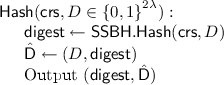
• $(\mathsf {digest}, \hat{\mathsf {D}}) \leftarrow \mathsf {Hash}(\mathsf {crs},D).$ It takes as input a common reference string $\mathsf {crs}$ and a database $D\in \{0,1\}^*$ and outputs a digest $\mathsf {digest}$ of the database and a state $\hat{\mathsf {D}}$.

• $\mathsf {e}\leftarrow \mathsf {Send}(\mathsf {crs},\mathsf {digest},L,m_0,m_1)$. It takes as input a common reference string $\mathsf {crs}$, a digest $\mathsf {digest}$, a database location $L\in \mathbb {N}$ and two messages $m_0$ and $m_1$ of length $\lambda$, and outputs a ciphertext $\mathsf {e}$.

• $m \leftarrow \mathsf {Receive}^{\hat{\mathsf {D}}}( \mathsf {crs}, \mathsf {e}, L)$. This is a RAM algorithm with random read access to $\hat{\mathsf {D}}$. It takes as input a common reference string $\mathsf {crs}$, a ciphertext $\mathsf {e}$, and a database location $L\in \mathbb {N}$. It outputs a message m.

We require the following properties of an $\ell OT$ scheme $(\mathsf {crsGen},\mathsf {Hash},\mathsf {Send},\mathsf {Receive})$.

• Correctness: We require that it holds for any database $D$ of size at most $M= \mathsf {poly}(\lambda )$ for any polynomial function $\mathsf {poly}(\cdot )$, any memory location $L\in [M]$, and any pair of messages $(m_0,m_1) \in \{0,1\} ^\lambda \times \{0,1\} ^\lambda$ that

  $$\begin{aligned} \Pr \left[ m = m_{D[L]} \begin{array}{|cl} \mathsf {crs}&{}\leftarrow \mathsf {crsGen}(1^\lambda )\\ (\mathsf {digest}, \hat{\mathsf {D}}) &{}\leftarrow \mathsf {Hash}(\mathsf {crs},D)\\ \mathsf {e}&{}\leftarrow \mathsf {Send}( \mathsf {crs}, \mathsf {digest}, L, m_0, m_1)\\ m &{}\leftarrow \mathsf {Receive}^{\hat{\mathsf {D}}}(\mathsf {crs}, \mathsf {e}, L) \end{array} \right] = 1, \end{aligned}$$

  where the probability is taken over the random choices made by $\mathsf {crsGen}$ and $\mathsf {Send}$.

• Sender Privacy Against Semi-Honest Receivers: There exists a PPT simulator $\mathsf {{\ell }OTSim}$ such that the following holds. For any database $D$ of size at most $M= \mathsf {poly}(\lambda )$ for any polynomial function $\mathsf {poly}(\cdot )$, any memory location $L\in [M]$, and any pair of messages $(m_0,m_1) \in \{0,1\} ^\lambda \times \{0,1\} ^\lambda$, let $\mathsf {crs}\leftarrow \mathsf {crsGen}(1^\lambda )$ and $\mathsf {digest}\leftarrow \mathsf {Hash}(\mathsf {crs},D)$. Then it holds that

  $$ \left( \mathsf {crs},\mathsf {Send}(\mathsf {crs},\mathsf {digest},L,m_0,m_1)\right) \mathop {\approx }\limits ^\mathrm{c}\left( \mathsf {crs}, \mathsf {{\ell }OTSim}(D, L, m_{D[L]})\right) . $$

• Efficiency Requirement: The length of $\mathsf {digest}$ is a fixed polynomial in $\lambda$ independent of the size of the database; we will assume for simplicity that $| \mathsf {digest}| = \lambda$. Moreover, the algorithm $\mathsf {Hash}$ runs in time $|D|\cdot \mathsf {poly}(\log |D|,\lambda )$, $\mathsf {Send}$ and $\mathsf {Receive}$ run in time $\mathsf {poly}(\log |D|,\lambda )$.

Receiver Privacy. In the above definition, we do not require receiver privacy as opposed to standard oblivious transfer, namely, no security guarantee is provided against a cheating (semi-honest) sender. This is mostly for ease of exposition. We would like to point out that adding receiver privacy (i.e., standard simulation based security against a semi-honest sender) to laconic OT can be done in a straightforward way. Instead of sending $\mathsf {digest}$ directly from the receiver to the sender and sending $\mathsf {e}$ back to the receiver, the two parties compute $\mathsf {Send}$ together via a two-round secure 2PC protocol, where the input of the receiver is $\mathsf {digest}$ and the input of the sender is $(L, m_0, m_1)$, and only the receiver obtains the output $\mathsf {e}$. This can be done using standard two-message OT and garbled circuits.

Multiple executions of $\mathsf {Send}$ that share the same $\mathsf {digest}$ . Notice that since the common reference string is public (i.e., not chosen by the simulator), the sender can involve $\mathsf {Send}$ function multiple times while still ensuring that security can be argued from the above definition (for the case of single execution) via a standard hybrid argument.

It will be convenient to use the following shorthand notations (generalizing the above notions) to run laconic OT for every single element in a database. Let $\mathsf {Keys}= ((\mathsf {Key}_{1,0},\mathsf {Key}_{1,1}),\dots ,(\mathsf {Key}_{M,0},\mathsf {Key}_{M,1}))$ be a list of $M= |D|$ key-pairs, where each key is of length $\lambda$. Then we will define

$$\begin{aligned}&\mathsf {Send}(\mathsf {crs},\mathsf {digest},\mathsf {Keys}) \\&= \left( \mathsf {Send}(\mathsf {crs},\mathsf {digest},1,\mathsf {Key}_{1,0},\mathsf {Key}_{1,1}),\dots ,\mathsf {Send}(\mathsf {crs},\mathsf {digest},M,\mathsf {Key}_{M,0},\mathsf {Key}_{M,1})\right) . \end{aligned}$$

Likewise, for a vector $\mathsf {e}= (\mathsf {e}_1,\dots ,\mathsf {e}_M)$ of ciphertexts define

$$ \mathsf {Receive}^{\hat{\mathsf {D}}}(\mathsf {crs},\mathsf {e}) = \left( \mathsf {Receive}^{\hat{\mathsf {D}}}(\mathsf {crs},\mathsf {e}_1,1),\dots ,\mathsf {Receive}^{\hat{\mathsf {D}}}(\mathsf {crs},\mathsf {e}_M,M)\right) . $$

Similarly, let $\mathsf {Labels}= \mathsf {Keys}_{D}=(\mathsf {Key}_{1, D[1]}, \dots , \mathsf {Key}_{M, D[M]})$, and define

$$\begin{aligned}&\mathsf {{\ell }OTSim}(\mathsf {crs}, D, \mathsf {Labels}) \\&= \left( \mathsf {{\ell }OTSim}(\mathsf {crs}, D, 1,\mathsf {Key}_{1, D[1]}), \dots , \mathsf {{\ell }OTSim}(\mathsf {crs}, D, M, \mathsf {Key}_{M, D[M]} \right) . \end{aligned}$$

By the sender security for multiple executions, we have that

$$ \left( \mathsf {crs}, \mathsf {Send}(\mathsf {crs},\mathsf {digest},\mathsf {Keys})\right) \mathop {\approx }\limits ^\mathrm{c}\left( \mathsf {crs},\mathsf {{\ell }OTSim}(\mathsf {crs}, D, \mathsf {Labels})\right) . $$

3.2 Updatable Laconic OT

For our applications, we will need a version of laconic OT for which the receiver’s short commitment $\mathsf {digest}$ to his database can be updated quickly (in time much smaller than the size of the database) when a bit of the database changes. We call this primitive supporting this functionality updatable laconic OT and define more formally below. At a high level, updatable laconic OT comes with an additional pair of algorithms $\mathsf {SendWrite}$ and $\mathsf {ReceiveWrite}$ which transfer the keys for an updated digest $\mathsf {digest}^*$ to the receiver. For convenience, we will define $\mathsf {ReceiveWrite}$ such that it also performs the write in $\hat{\mathsf {D}}$.

Definition 2

(Updatable Laconic OT). An updatable laconic OT (updatable $\ell OT$) scheme consists of algorithms $\mathsf {crsGen}, \mathsf {Hash}, \mathsf {Send}, \mathsf {Receive}$ as per Definition 1 and additionally two algorithms $\mathsf {SendWrite}$ and $\mathsf {ReceiveWrite}$ with the following syntax.

• $\mathsf {e_w}\leftarrow \mathsf {SendWrite}\left( \mathsf {crs},\mathsf {digest},L,b, \left\{ m_{j,0}, m_{j,1}\right\} _{j=1}^{|\mathsf {digest}|}\right)$. It takes as input the common reference string $\mathsf {crs}$, a digest $\mathsf {digest}$, a location $L\in \mathbb {N}$, a bit $b \in {\{0,1\}}$ to be written, and $|\mathsf {digest}|$ pairs of messages $\left\{ m_{j,0}, m_{j,1}\right\} _{j=1}^{|\mathsf {digest}|}$, where each $m_{j,c}$ is of length $\lambda$. And it outputs a ciphertext $\mathsf {e_w}$.

• $\{m_j\}_{j=1}^{|\mathsf {digest}|} \leftarrow \mathsf {ReceiveWrite}^{\hat{\mathsf {D}}}(\mathsf {crs}, L, b, \mathsf {e_w})$. This is a RAM algorithm with random read/write access to $\hat{\mathsf {D}}$. It takes as input the common reference string $\mathsf {crs}$, a location $L$, a bit $b \in {\{0,1\}}$ and a ciphertext $\mathsf {e_w}$. It updates the state ${\hat{\mathsf {D}}}$ (such that $D[L] = b$) and outputs messages $\{m_j\}_{j=1}^{|\mathsf {digest}|}$.

We require the following properties on top of properties of a laconic OT scheme.

• Correctness With Regard To Writes: For any database $D$ of size at most $M= \mathsf {poly}(\lambda )$ for any polynomial function $\mathsf {poly}(\cdot )$, any memory location $L\in [M]$, any bit $b \in {\{0,1\}}$, and any messages $\left\{ m_{j,0}, m_{j,1}\right\} _{j=1}^{|\mathsf {digest}|}$ of length $\lambda$, the following holds. Let $D^*$ be identical to $D$, except that $D^*[L] = b$,

  $$ \Pr \left[ \begin{array}{l} m_j' = m_{j,\mathsf {digest}^*_{j}}\\ \forall j\in [|\mathsf {digest}|] \end{array} \begin{array}{|cl} \mathsf {crs}&{}\leftarrow \mathsf {crsGen}(1^\lambda )\\ (\mathsf {digest}, \hat{\mathsf {D}}) &{}\leftarrow \mathsf {Hash}(\mathsf {crs},D)\\ (\mathsf {digest}^*, \hat{\mathsf {D}}^*) &{}\leftarrow \mathsf {Hash}(\mathsf {crs},D^*)\\ \mathsf {e_w}&{} \leftarrow \mathsf {SendWrite}\left( \mathsf {crs},\mathsf {digest},L,b, \left\{ m_{j,0}, m_{j,1}\right\} _{j=1}^{|\mathsf {digest}|}\right) \\ \{m_j'\}_{j=1}^{|\mathsf {digest}|} &{} \leftarrow \mathsf {ReceiveWrite}^{\hat{\mathsf {D}}}( \mathsf {crs}, L, b, \mathsf {e_w}) \end{array} \right] = 1, $$

  where the probability is taken over the random choices made by $\mathsf {crsGen}$ and $\mathsf {SendWrite}$. Furthermore, we require that the execution of $\mathsf {ReceiveWrite}^{\hat{\mathsf {D}}}$ above updates ${\hat{\mathsf {D}}}$ to $\hat{\mathsf {D}}^*$. (Note that $\mathsf {digest}$ is included in $\hat{\mathsf {D}}$, hence $\mathsf {digest}$ is also updated to $\mathsf {digest}^*$.)

• Sender Privacy Against Semi-Honest Receivers With Regard To Writes: There exists a PPT simulator $\mathsf {{\ell }OTSimWrite}$ such that the following holds. For any database $D$ of size at most $M= \mathsf {poly}(\lambda )$ for any polynomial function $\mathsf {poly}(\cdot )$, any memory location $L\in [M]$, any bit $b \in {\{0,1\}}$, and any messages $\left\{ m_{j,0}, m_{j,1}\right\} _{j=1}^{|\mathsf {digest}|}$ of length $\lambda$, let $\mathsf {crs}\leftarrow \mathsf {crsGen}(1^\lambda )$, $(\mathsf {digest}, \hat{\mathsf {D}}) \leftarrow \mathsf {Hash}(\mathsf {crs},D)$, and $(\mathsf {digest}^*, \hat{\mathsf {D}}^*) \leftarrow \mathsf {Hash}(\mathsf {crs},D^*)$, where $D^*$ is identical to $D$ except that $D^*[L] = b$. Then it holds that

  $$ \begin{array}{rl} &{}\left( \mathsf {crs},\mathsf {SendWrite}(\mathsf {crs},\mathsf {digest},L,b,\left\{ m_{j,0}, m_{j,1}\right\} _{j=1}^{|\mathsf {digest}|})\right) \\ \mathop {\approx }\limits ^\mathrm{c}&{} \left( \mathsf {crs},\mathsf {{\ell }OTSimWrite}\left( \mathsf {crs}, D, L, b, \{m_{j,\mathsf {digest}^*_{j}}\}_{j\in [|\mathsf {digest}|]}\right) \right) . \end{array} $$

• Efficiency Requirements: We require that both $\mathsf {SendWrite}$ and $\mathsf {ReceiveWrite}$ run in time $\mathsf {poly}(\log |D|,\lambda )$.

4 Laconic Oblivious Transfer with Factor-2 Compression

In this section, based on the DDH assumption we will construct a laconic OT scheme for which the hash function $\mathsf {Hash}$ compresses a database of length $2\lambda$ into a digest of length $\lambda$. We would refer to this primitive as laconic OT with factor-2 compression. We note that, subsequent to our work, the factor-2 compression construction has been simplified by Döttling and Garg [DG17] (another alternative simplification can be obtained using [AIKW13]). We refer the reader to [DG17] for the simpler construction and preserve the older construction here.

We will first construct the following two primitives as building blocks: (1) a somewhere statistically binding (SSB) hash function, and (2) a hash proof system that allows for proving knowledge of preimage bits for this SSB hash function. We will then present the $\ell OT$ scheme with factor-2 compression in Sect. 4.4.

4.1 Somewhere Statistically Binding Hash Functions and Hash Proof Systems

In this section, we give definitions of somewhere statistically binding (SSB) hash functions [HW15] and hash proof systems [CS98]. For simplicity, we will only define SSB hash functions that compress $2 \lambda$ values in the domain into $\lambda$ bits. The more general definition works analogously.

Definition 3

(Somewhere Statistically Binding Hashing). An SSB hash function $\mathsf {SSBH}$ consists of three algorithms $\mathsf {crsGen}$, $\mathsf {bindingCrsGen}$ and $\mathsf {Hash}$ with the following syntax.

• $\mathsf {crs}\leftarrow \mathsf {crsGen}(1^\lambda )$. It takes the security parameter $\lambda$ as input and outputs a common reference string $\mathsf {crs}$.

• $\mathsf {crs}\leftarrow \mathsf {bindingCrsGen}(1^\lambda ,i)$. It takes as input the security parameter $\lambda$ and an index $i \in [2 \lambda ]$, and outputs a common reference string $\mathsf {crs}$.

• $y \leftarrow \mathsf {Hash}(\mathsf {crs},x)$. For some domain $\mathfrak {D}$, it takes as input a common reference string $\mathsf {crs}$ and a string $x \in \mathfrak {D}^{2\lambda }$, and outputs a string $y \in \{0,1\} ^\lambda$.

We require the following properties of an SSB hash function.

• Statistically Binding at Position i : For every $i \in [2\lambda ]$ and an overwhelming fraction of $\mathsf {crs}$ in the support of $\mathsf {bindingCrsGen}(1^\lambda ,i)$ and every $x \in \mathfrak {D}^{2\lambda }$, we have that $(\mathsf {crs},\mathsf {Hash}(\mathsf {crs},x))$ uniquely determines $x_i$. More formally, for all $x' \in \mathfrak {D}^{2\lambda }$ such that $x_i \ne x_i'$ we have that $\mathsf {Hash}(\mathsf {crs},x')\ne \mathsf {Hash}(\mathsf {crs},x)$.

• Index Hiding: It holds for all $i \in [2 \lambda ]$ that $\mathsf {crsGen}(1^\lambda ) \mathop {\approx }\limits ^\mathrm{c}\mathsf {bindingCrsGen}(1^\lambda ,i)$, i.e., common reference strings generated by $\mathsf {crsGen}$ and $\mathsf {bindingCrsGen}$ are computationally indistinguishable.

Next, we define hash proof systems [CS98] that are designated verifier proof systems that allow for proving that the given problem instance in some language. We give the formal definition as follows.

Definition 4

(Hash Proof System). Let $\mathcal {L}_z \subseteq \mathcal {M}_z$ be an NP-language residing in a universe $\mathcal {M}_z$, both parametrized by some parameter z. Moreover, let $\mathcal {L}_z$ be characterized by an efficiently computable witness-relation $\mathcal {R}$, namely, for all $x \in M_z$ it holds that $x \in \mathcal {L}_z \Leftrightarrow \exists w: \mathcal {R}(x,w) = 1$. A hash proof system $\mathsf {HPS}$ for $\mathcal {L}_z$ consists of three algorithms $\mathsf {KeyGen}$, $\mathsf {H_{public}}$ and $\mathsf {H_{secret}}$ with the following syntax.

• $(\mathsf {pk}, \mathsf {sk}) \leftarrow \mathsf {KeyGen}(1^\lambda , z)$: Takes as input the security parameter $\lambda$ and a parameter z, and outputs a public-key and secret key pair $(\mathsf {pk},\mathsf {sk})$.

• $y \leftarrow \mathsf {H_{public}}(\mathsf {pk},x,w)$: Takes as input a public key $\mathsf {pk}$, an instance $x \in \mathcal {L}_z$, and a witness w, and outputs a value y.

• $y \leftarrow \mathsf {H_{secret}}(\mathsf {sk},x)$: Takes as input a secret key $\mathsf {sk}$ and an instance $x \in M_z$, and outputs a value y.

We require the following properties of a hash proof system.

• Perfect Completeness: For every z, every $(\mathsf {pk},\mathsf {sk})$ in the support of $\mathsf {KeyGen}(1^\lambda , z)$, and every $x \in \mathcal {L}_z$ with witness w (i.e., $\mathcal {R}(x,w) = 1$), it holds that

  $$ \mathsf {H_{public}}(\mathsf {pk},x,w) = \mathsf {H_{secret}}(\mathsf {sk},x). $$

• Perfect Soundness: For every z and every $x \in M_z \setminus \mathcal {L}_z$, let $(\mathsf {pk},\mathsf {sk})\leftarrow \mathsf {KeyGen}(1^\lambda , z)$, then it holds that

  $$ (z, \mathsf {pk}, \mathsf {H_{secret}}(\mathsf {sk},x)) \equiv (z, \mathsf {pk}, u), $$

  where u is distributed uniformly random in the range of $\mathsf {H_{secret}}$. Here, $\equiv$ denotes distributional equivalence.

4.2 HPS-friendly SSB Hashing

In this section, we will construct an HPS-friendly SSB hash function that supports a hash proof system. In particular, there is a hash proof system that enables proving that a certain bit of the pre-image of a hash-value has a certain fixed value (in our case, either 0 or 1).

We start with some notations. Let $(\mathbb {G},\cdot )$ be a cyclic group of order p with generator g. Let $\mathbf {M} \in \mathbb {Z}_p^{m \times n}$ be a matrix. We will denote by $\hat{\mathbf {M}} = g^{\mathbf {M}} \in \mathbb {G}^{m \times n}$ the element-wise exponentiation of g with the elements of $\mathbf {M}$. We also define $\hat{\mathbf {L}} = \hat{\mathbf {H}}^{\mathbf {M}} \in \mathbb {G}^{m\times k}$, where $\hat{\mathbf {H}} \in \mathbb {G}^{m \times n}$ and $\mathbf {M} \in \mathbb {Z}_p^{n \times k}$ as follows: Each element $\hat{\mathbf {L}}_{i,j} = \prod _{k = 1}^n \hat{\mathbf {H}}_{i,k}^{\mathbf {M}_{k,j}}$ (intuitively this operation corresponds to matrix multiplication in the exponent). This is well-defined and efficiently computable.

Computational Assumptions. In the following, we first define the computational problems on which we will base the security of our HPS-friendly SSB hash function.

Definition 5

(The Decisional Diffie-Hellman (DDH) Problem). Let $(\mathbb {G},\cdot )$ be a cyclic group of prime order p and with generator g. Let a, b, c be sampled uniformly at random from $\mathbb {Z}_p$ (i.e., $a,b,c \xleftarrow {\$}\mathbb {Z}_p$). The DDH problem asks to distinguish the distributions $(g,g^a,g^b,g^{ab})$ and $(g,g^a,g^b,g^c)$.

Definition 6

(Matrix Rank Problem). Let m, n be integers and let $\mathbb {Z}_p^{m \times n; r}$ be the set of all $m \times n$ matrices over $\mathbb {Z}_p$ with rank r. Further, let $1 \le r_1 < r_2 \le \min (m,n)$. The goal of the matrix rank problem, denoted as $\mathsf {MatrixRank}(\mathbb {G},m,n,r_1,r_2)$, is to distinguish the distributions $g^{\mathbf {M}_1}$ and $g^{\mathbf {M}_2}$, where $\mathbf {M}_1 \xleftarrow {\$}\mathbb {Z}_p^{m \times n; r_1}$ and $\mathbf {M}_2 \xleftarrow {\$}\mathbb {Z}_p^{m \times n; r_2}$.

In a recent result by Villar [Vil12] it was shown that the matrix rank problem can be reduced almost tightly to the DDH problem.

Theorem 1

([Vil12] Theorem 1, simplified). Assume there exists a PPT distinguisher $\mathcal {D}$ that solves $\mathsf {MatrixRank}(\mathbb {G},m,n,r_1,r_2)$ problem with advantage $\epsilon$. Then, there exists a PPT distinguisher $\mathcal {D}'$ (running in almost time as $\mathcal {D}$) that solves $\mathsf {DDH}$ problem over $\mathbb {G}$ with advantage at least $\frac{\epsilon }{\lceil \log _2(r_2 / r_1)\rceil }$.

We next give the construction of an HPS-friendly SSB hash function.

Construction. Our construction builds on the scheme of Okamoto et al. [OPWW15]. We will not delve into the details of their scheme and directly jump into our construction.

Let n be an integer such that $n = 2\lambda$, and let $(\mathbb {G},\cdot )$ be a cyclic group of order p and with generator g. Let $\mathbf {T}_i \in \mathbb {Z}_p^{2 \times n}$ be a matrix which is zero everywhere except the i-th column, and the i-th column is equal to $\mathbf {t} = (0,1)^\top$. The three algorithms of the SSB hash function are defined as follows.

• $\mathsf {crsGen}(1^\lambda )$: Pick a uniformly random matrix $\mathbf {H} \xleftarrow {\$}\mathbb {Z}_p^{2 \times n}$ and output $\hat{\mathbf {H}} = g^{\mathbf {H}}$.

• $\mathsf {bindingCrsGen}(1^\lambda ,i)$: Pick a uniformly random vector $(w_1, w_2)^\top = \mathbf {w} \xleftarrow {\$}\mathbb {Z}_p^2$ with the restriction that $w_1 = 1$, pick a uniformly random vector $\mathbf {a} \xleftarrow {\$}\mathbb {Z}_p^n$ and set $\mathbf {A} \leftarrow \mathbf {w} \cdot \mathbf {a}^\top$. Set $\mathbf {H} \leftarrow \mathbf {T}_i + \mathbf {A}$ and output $\hat{\mathbf {H}} = g^{\mathbf {H}}$.

• $\mathsf {Hash}(\mathsf {crs},\mathbf {x})$: Parse $\mathbf {x}$ as a vector in $\mathfrak {D}^n$ ($\mathfrak {D}= \mathbb {Z}_p$) and parse $\mathsf {crs}= \hat{\mathbf {H}}$. Compute $\mathbf {y}\in \mathbb {G}^2$ as $\mathbf {y} = \hat{\mathbf {H}}^\mathbf {x}$. Parse $\mathbf {y}$ as a binary string and output the result.

Compression. Notice that we can get factor two compression for an input space $\{0,1\} ^{2\lambda }$ by restricting the domain to $\mathfrak {D}' = \{0,1\} \subset \mathfrak {D}$. The input length $n= 2\lambda$, where $\lambda$ is set to be twice the number of bits in the bit representation of a group element in $\mathbb {G}$. In the following we will assume that $n=2\lambda$ and that the bit-representation size of a group element in $\mathbb {G}$ is $\frac{\lambda }{2}$.

We will first show that the distributions $\mathsf {crsGen}(1^\lambda )$ and $\mathsf {bindingCrsGen}(1^\lambda ,i)$ are computationally indistinguishable for every index $i \in [n]$, given that the DDH problem is computationally hard in the group $\mathbb {G}$.

Lemma 1

(Index Hiding). Assume that the $\mathsf {MatrixRank}(\mathbb {G},2,n,1,2)$ problem is hard. Then the distributions $\mathsf {crsGen}(1^\lambda )$ and $\mathsf {bindingCrsGen}(1^\lambda ,i)$ are computationally indistinguishable, for every $i \in [n]$.

Proof

Assume there exists a PPT distinguisher $\mathcal {D}$ that distinguishes the distributions $\mathsf {crsGen}(1^\lambda )$ and $\mathsf {bindingCrsGen}(1^\lambda ,i)$ with non-negligible advantage $\epsilon$. We will construct a PPT distinguisher $\mathcal {D}'$ that distinguishes $\mathsf {MatrixRank}(\mathbb {G},2,n,1,2)$ with non-negligible advantage.

The distinguisher $\mathcal {D}'$ does the following on input $\hat{\mathbf {M}} \in \mathbb {G}^{2 \times n}$. It computes $\hat{\mathbf {H}} \in \mathbb {G}^{2\times n}$ as element-wise multiplication of $\hat{\mathbf {M}}$ and $g^{ \mathbf {T}_i}$ and runs $\mathcal {D}$ on $\hat{\mathbf {H}}$. If $\mathcal {D}$ outputs $\mathsf {crsGen}$, then $\mathcal {D'}$ outputs rank 2, otherwise $\mathcal {D'}$ outputs rank 1.

We will now show that $\mathcal {D}'$ also has non-negligible advantage. Write $\mathcal {D}'$’s input as $\hat{\mathbf {M}} = g^{\mathbf {M}}$. If $\mathbf {M}$ is chosen uniformly random with rank 2, then $\mathbf {M}$ is uniform in $\mathbb {Z}_p^{2 \times n}$ with overwhelming probability. Hence with overwhelming probability, $\mathbf {M} + \mathbf {T}_i$ is also distributed uniformly random and it follows that $\hat{\mathbf {H}} = g^{\mathbf {M} + \mathbf {T}_i}$ is uniformly random in $\mathbb {G}^{2 \times n}$ which is identical to the distribution generated by $\mathsf {crsGen}(1^\lambda )$. On the other hand, if $\mathbf {M}$ is chosen uniformly random with rank 1, then there exists a vector $\mathbf {w} \in \mathbb {Z}_p^2$ such that each column of $\mathbf {M}$ can be written as $a_i \cdot \mathbf {w}$. We can assume that the first element $w_1$ of $\mathbf {w}$ is 1, since the case $w_1 = 0$ happens only with probability $1/p = \mathsf {negl}(\lambda )$ and if $w_1 \ne 0$ we can replace all $a_i$ by $a'_i = a_i\cdot w_1$ and replace $w_i$ by $w_i' = \frac{w_i}{w_1}$. Thus, we can write $\mathbf {M}$ as $\mathbf {M} = \mathbf {w} \cdot \mathbf {a}^\top$ and consequently $\hat{\mathbf {H}}$ as $\hat{\mathbf {H}} = g^{\mathbf {w} \cdot \mathbf {a}^\top + \mathbf {T}_i}$. Notice that $\mathbf {a}$ is uniformly distributed, hence $\hat{\mathbf {H}}$ is identical to the distribution generated by $\mathsf {bindingCrsGen}(1^\lambda ,i)$. Since $\mathcal {D}$ can distinguish the distributions $\mathsf {crsGen}(1^\lambda )$ and $\mathsf {bindingCrsGen}(1^\lambda ,i)$ with non-negligible advantage $\epsilon$, $\mathcal {D}'$ can distinguish $\mathsf {MatrixRank}(\mathbb {G},2,n,1,2)$ with advantage $\epsilon - \mathsf {negl}(\lambda )$, which contradicts the hardness of $\mathsf {MatrixRank}(\mathbb {G},2,n,1,2)$.

A corollary of Lemma 1 is that for all $i,j \in [n]$ the distributions $\mathsf {bindingCrsGen}(1^\lambda ,i)$ and $\mathsf {bindingCrsGen}(1^\lambda ,j)$ are indistinguishable, stated as follows.

Corollary 1

Assume the $\mathsf {MatrixRank}(\mathbb {G},2,n,1,2)$ problem is computationally hard. Then it holds for all $i,j \in [n]$ that $\mathsf {bindingCrsGen}(1^\lambda ,i)$ and $\mathsf {bindingCrsGen}(1^\lambda ,j)$ are computationally indistinguishable.

We next show that if the common reference string $\mathsf {crs}= \hat{\mathbf {H}}$ is generated by $\mathsf {bindingCrsGen}(1^\lambda ,i)$, then the hash value $\mathsf {Hash}(\mathsf {crs},\mathbf {x})$ is statistically binded to $x_i$.

Lemma 2

(Statistically Binding at Position i ). For every $i \in [n]$, every $\mathbf {x} \in \mathbb {Z}_p^n$, and all choices of $\mathsf {crs}$ in the support of $\mathsf {bindingCrsGen}(1^\lambda ,i)$ we have that for every $\mathbf {x}' \in \mathbb {Z}_p^n$ such that ${x}_i' \ne {x}_i$, $\mathsf {Hash}(\mathsf {crs}, \mathbf {x}) \ne \mathsf {Hash}(\mathsf {crs},\mathbf {x}')$.

Proof

We first write $\mathsf {crs}$ as $\hat{\mathbf {H}} = g^{\mathbf {H}} = g^{\mathbf {w} \cdot \mathbf {a}^\top + \mathbf {T}_i}$ and $\mathsf {Hash}(\mathsf {crs},\mathbf {x})$ as $\mathsf {Hash}(\hat{\mathbf {H}},\mathbf {x}) = g^{\mathbf {y}} = g^{\mathbf {H} \cdot \mathbf {x}}$. Thus, by taking the discrete logarithm with basis g our task is to demonstrate that there exists a unique $x_i$ from $\mathbf {H} = \mathbf {w} \cdot \mathbf {a}^\top + \mathbf {T}_i$ and $\mathbf {y} = \mathbf {H} \cdot \mathbf {x}$. Observe that

$$\begin{aligned} \mathbf {y}&= \mathbf {H} \cdot \mathbf {x} = (\mathbf {w} \cdot \mathbf {a}^\top + \mathbf {T}_i) \cdot \mathbf {x} = \mathbf {w} \cdot \langle \mathbf {a}, \mathbf {x} \rangle + \mathbf {T}_i \cdot \mathbf {x} \\&= \left( \begin{matrix} 1 \\ w_2 \end{matrix} \right) \cdot \langle \mathbf {a}, \mathbf {x} \rangle + \left( \begin{matrix} 0 \\ 1 \end{matrix} \right) \cdot x_i, \end{aligned}$$

where $\langle \mathbf {a}, \mathbf {x} \rangle$ is the inner product of $\mathbf {a}$ and $\mathbf {x}$. If $\mathbf {a}\ne \mathbf {0}$, then we can use any non-zero element of $\mathbf {a}$ to compute $w_2$ from $\mathbf {H}$, and recover $x_i$ by computing $x_i = y_2 - w_2 \cdot y_1$; otherwise $\mathbf {a}=\mathbf {0}$, so $x_i = y_2$.

4.3 A Hash Proof System for Knowledge of Preimage Bits

In this section, we give our desired hash proof systems. In particular, we need a hash proof system for membership in a subspace of a vector space. In our proof we need the following technical lemma.

Lemma 3

Let $\mathbf {M} \in \mathbb {Z}_p^{{m} \times n}$ be a matrix. Let $\mathsf {colsp}(\mathbf {M}) = \{ \mathbf {M} \cdot \mathbf {x} \ | \ \mathbf {x} \in \mathbb {Z}_p^n \}$ be its column space, and $\mathsf {rowsp}(\mathbf {M}) = \{ \mathbf {x}^\top \cdot \mathbf {M} \ | \ \mathbf {x} \in \mathbb {Z}_p^m \}$ be its row space. Assume that $\mathbf {y} \in \mathbb {Z}_p^m$ and $\mathbf {y} \notin \mathsf {colsp}(\mathbf {M})$. Let $\mathbf {r} \xleftarrow {\$}\mathbb {Z}_p^m$ be chosen uniformly at random. Then it holds that

$$ ( \mathbf {M},\mathbf {y}, \mathbf {r}^\top \mathbf {M}, \mathbf {r}^\top \mathbf {y}) \equiv (\mathbf {M},\mathbf {y}, \mathbf {r}^\top \mathbf {M}, u), $$

where $u \xleftarrow {\$}\mathbb {Z}_p$ is distributed uniformly and independently of $\mathbf {r}$. Here, $\equiv$ denotes distributional equivalence.

Proof

For any $\mathbf {t} \in \mathsf {rowsp}(\mathbf {M})$ and $s \in \mathbb {Z}_p$, consider following linear equation system

$$\begin{aligned} \left\{ \begin{array}{l} \mathbf {r}^\top \mathbf {M} = \mathbf {t} \\ \mathbf {r}^\top \mathbf {y} = s \end{array} \right. . \end{aligned}$$

Let $\mathcal {N}$ be the left null space of $\mathbf {M}$. We know that $\mathbf {y} \notin \mathsf {colsp}(\mathbf {M})$, hence $\mathbf {M}$ has rank $\le m-1$, therefore $\mathcal {N}$ has dimension ${\ge }1$. Let $\mathbf {r}_0$ be an arbitrary solution for $\mathbf {r}^\top \mathbf {M} = \mathbf {t}$, and let $\mathbf {n}$ be a vector in $\mathcal {N}$ such that $\mathbf {n}^\top \mathbf {y} \ne \mathbf {0}$ (there must be such a vector since $\mathbf {y} \notin \mathsf {colsp}(\mathbf {M})$). Then there exists a solution $\mathbf {r}$ for the above linear equation system, that is,

$$\begin{aligned} \mathbf {r} = \mathbf {r}_0 + (\mathbf {n}^\top \mathbf {y})^{-1} \cdot (s-\mathbf {r}_0^\top \mathbf {y}) \cdot \mathbf {n}, \end{aligned}$$

where $(\mathbf {n}^\top \mathbf {y})^{-1}$ is the multiplicative inverse of $\mathbf {n}^\top \mathbf {y}$ in $\mathbb {Z}_p$. Then two cases arise: (i) column vectors of $\left( \mathbf {M} \ \mathbf {y} \right)$ are full-rank, or (ii) not. In this first case, there is a unique solution for $\mathbf {r}$. In the second case the solution space has the same size as the left null space of $\left( \mathbf {M} \ \mathbf {y} \right)$. Therefore, in both cases, the number of solutions for $\mathbf {r}$ is the same for every $(\mathbf {t},s)$ pair.

As $\mathbf {r}$ is chosen uniformly at random, all pairs $(\mathbf {t},s) \in \mathsf {rowsp}(\mathbf {M}) \times \mathbb {Z}_p$ have the same probability of occurrence and the claim follows.

Construction. Fix a matrix $\hat{\mathbf {H}} \in \mathbb {G}^{2 \times n}$ and an index $i \in [n]$. We will construct a hash proof system $\mathsf {HPS} = (\mathsf {KeyGen}, \mathsf {H_{public}}, \mathsf {H_{secret}})$ for the following language $\mathcal {L}_{\hat{\mathbf {H}},i}$:

$$ \mathcal {L}_{\hat{\mathbf {H}},i} = \{ (\hat{\mathbf {y}},b) \in \mathbb {G}^{2} \times {\{0,1\}}\ | \ \exists \mathbf {x} \in \mathbb {Z}_p^n \text { s.t. } \hat{\mathbf {y}} = \hat{\mathbf {H}}^{\mathbf {x}} \text { and } x_i = b \}. $$

Note that in our hash proof system we only enforce that a single specified bit is b, where $b \in \{0,1\}$. However, our hash proof system does not place any requirement on the value used at any of the other locations. In fact the values used at the other locations may actually be from the full domain $\mathfrak {D}$ (i.e., $\mathbb {Z}_p$). Observe that the formal definition of the language $\mathcal {L}_{\hat{\mathbf {H}},i}$ above incorporates this difference in how the honest computation of the hash function is performed and what the hash proof system is supposed to prove.

For ease of exposition, it will be convenient to work with a matrix $\hat{\mathbf {H}}' \in \mathbb {G}_p^{3 \times n}$:

where $\mathbf {e}_i \in \mathbb {Z}_p^n$ is the i-th unit vector, with all elements equal to zero except the $i^{th}$ one which is equal to one.

• $\mathsf {KeyGen}(1^\lambda , (\hat{\mathbf {H}},i))$: Choose $\mathbf {r} \xleftarrow {\$}\mathbb {Z}_p^{3}$ uniformly at random. Compute $\hat{\mathbf {h}} = \left( (\hat{\mathbf {H}}')^\top \right) ^{\mathbf {r}}$. Set $\mathsf {pk} = \hat{\mathbf {h}}$ and $\mathsf {sk} = \mathbf {r}$. Output $(\mathsf {pk},\mathsf {sk})$.

• $\mathsf {H_{public}}(\mathsf {pk},(\hat{\mathbf {y}},b),\mathbf {x})$: Parse $\mathsf {pk}$ as $\hat{\mathbf {h}}$. Compute $\hat{z} = (\hat{\mathbf {h}}^\top )^{\mathbf {x}}$ and output $\hat{z}$.

• $\mathsf {H_{secret}}(\mathsf {sk},(\hat{\mathbf {y}},b) )$: Parse $\mathsf {sk}$ as $\mathbf {r}$ and set . Compute $\hat{z} = ((\hat{\mathbf {y}}')^\top )^{\mathbf {r}}$ and output $\hat{z}$.

Lemma 4

For every matrix $\hat{\mathbf {H}} \in \mathbb {G}^{2\times n}$ and every $i \in [n]$, $\mathsf {HPS}$ is a hash proof system for the language $\mathcal {L}_{\hat{\mathbf {H}},i}$.

Proof

Let $\hat{\mathbf {H}} = g^{\mathbf {H}}$, $\mathbf {r} = (\mathbf {r}^*,r_{3})$ where $\mathbf {r}^*\in \mathbb {Z}_p^2$. Let $\mathbf {y}':= \log _g \hat{\mathbf {y}}'$, $\mathbf {y} := \log _g \hat{\mathbf {y}}$, $\mathbf {H}':= \log _g \hat{\mathbf {H}}'$, $\mathbf {h} := \log _g \hat{\mathbf {h}}$.

For perfect correctness, we need to show that for every $i \in [n]$, every $\hat{\mathbf {H}} \in \mathbb {G}^{2\times n}$, and every $(\mathsf {pk},\mathsf {sk})$ in the support of $\mathsf {KeyGen}(1^\lambda , (\hat{\mathbf {H}}',i))$, if $(\hat{\mathbf {y}},b) \in \mathcal {L}_{\hat{\mathbf {H}},i}$ and $\mathbf {x}$ is a witness for membership (i.e., $\hat{\mathbf {y}} = \hat{\mathbf {H}}^{\mathbf {x}}$ and $x_i = b$), then it holds that $\mathsf {H_{public}}(\mathsf {pk},(\hat{\mathbf {y}},b),\mathbf {x}) = \mathsf {H_{secret}}(\mathsf {sk},(\hat{\mathbf {y}},b))$.

To simplify the argument, we again consider the statement under the discrete logarithm with basis g. Then it holds that

$$\begin{aligned}&\log _g\left( \mathsf {H_{secret}}(\mathsf {sk},(\hat{\mathbf {y}},b))\right) \\ =&\log _g\left( \left( (\hat{\mathbf {y}}')^\top \right) ^\mathbf {r} \right) = \langle \mathbf {y}', \mathbf {r} \rangle = \langle \mathbf {y}, \mathbf {r}^*\rangle + b \cdot r_3 \\ =&\langle \mathbf {H} \cdot \mathbf {x}, \mathbf {r}^*\rangle + x_i \cdot r_3 = \langle \mathbf {H}' \mathbf {x}, \mathbf {r} \rangle = \langle (\mathbf {H}')^\top \mathbf {r}, \mathbf {x} \rangle \\ =&\langle \mathbf {h}, \mathbf {x} \rangle = \log _g\left( (\hat{\mathbf {h}}^\top )^{\mathbf {x}}\right) \\ =&\log _g\left( \mathsf {H_{public}}(\mathsf {pk},(\hat{\mathbf {y}},b),\mathbf {x})\right) . \end{aligned}$$

For perfect soundness, let $(\mathsf {pk},\mathsf {sk})\leftarrow \mathsf {KeyGen}(1^\lambda , (\hat{\mathbf {H}}',i))$. We will show that if $(\hat{\mathbf {y}},b) \notin \mathcal {L}_{\hat{\mathbf {H}},i}$, then $\mathsf {H_{secret}}(\mathsf {sk},(\hat{\mathbf {y}},b))$ is distributed uniformly random in the range of $\mathsf {H_{secret}}$, even given $\hat{\mathbf {H}}$, i, and $\mathsf {pk}$. Again under the discrete logarithm, this is equivalent to showing that $\langle \mathbf {y}', \mathbf {r} \rangle$ is distributed uniformly random given $\mathbf {H}'$ and $\mathbf {h} = (\mathbf {H}')^\top \mathbf {r}$.

Note that we can re-write the language $\mathcal {L}_{\hat{\mathbf {H}},i} = \{ (\hat{\mathbf {y}},b) \in \mathbb {G}^{2} \times \mathbb {Z}_p \ | \ \exists \mathbf {x} \in \mathbb {Z}_p^n \text { s.t. } \mathbf {H'}\mathbf {x} = \mathbf {y}' \}$. It follows that if $(\hat{\mathbf {y}},b) \notin \mathcal {L}_{\hat{\mathbf {H}},i}$, then $\mathbf {y}' \notin \mathsf {span}(\mathbf {H}')$. Now it follows directly from Lemma 3 that

$$ \mathbf {r}^\top \mathbf {y}' \equiv u $$

given $\mathbf {H}'$ and $\mathbf {r}^\top \mathbf {H}'$, where u is distributed uniformly random. This concludes the proof.

Remark 1

While proving the security of our applications based on the above hash-proof system, we would generate $\hat{\mathbf {H}}$ to be the output of $\mathsf {bindingCrsGen}(1^\lambda ,i)$ and use the property that if $(\hat{\mathbf {y}}, b) \in \mathcal {L}_{\hat{\mathbf {H}},i}$, then $(\hat{\mathbf {y}}, (1-b)) \notin \mathcal {L}_{\hat{\mathbf {H}},i}$. This follows directly from Lemma 2 (that is, $\hat{\mathbf {H}}$ and $\hat{\mathbf {y}}$ uniquely fixes $x_i$).

4.4 The Laconic OT Scheme

We are now ready to put the pieces together and provide our $\ell OT$ scheme with factor-2 compression.

Construction. Let $\mathsf {SSBH}= (\mathsf {SSBH}.\mathsf {crsGen},\mathsf {SSBH}.\mathsf {bindingCrsGen},\mathsf {SSBH}.\mathsf {Hash})$ be the HPS-friendly SSB hash function constructed in Sect. 4.2 with domain $\mathfrak {D}=\mathbb {Z}_p$. Notice that we achieve factor-2 compression (namely, compressing $2\lambda$ bits into $\lambda$ bits) by restricting the domain from $\mathfrak {D}^n$ to ${\{0,1\} }^n$ in our laconic OT scheme. Also, abstractly let the associated hash proof system be $\mathsf {HPS} = (\mathsf {HPS.KeyGen}, \mathsf {HPS.H_{public}},\mathsf {HPS.H_{secret}})$ for the language

$$ \mathcal {L}_{\mathsf {crs},i} = \{ (\mathsf {digest},b) \in \{0,1\} ^{\lambda } \times \{0,1\} \ | \ \exists D\in \mathfrak {D}^{2\lambda } : \mathsf {SSBH}.\mathsf {Hash}(\mathsf {crs},D) = \mathsf {digest}\text { and } D[i] = b \}. $$

Recall that the bit-representation size of a group element of $\mathbb {G}$ is $\frac{\lambda }{2}$, hence the language defined above is the same as the one defined in Sect. 4.3.

Now we construct the laconic OT scheme $\ell OT= (\mathsf {crsGen}, \mathsf {Hash}, \mathsf {Send}, \mathsf {Receive})$ as follows.

• $\mathsf {crsGen}(1^\lambda )$: Compute $\mathsf {crs}\leftarrow \mathsf {SSBH}.\mathsf {crsGen}(1^\lambda )$ and output $\mathsf {crs}$.

• 

• 

• 

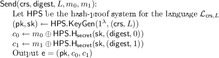
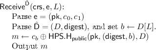
We will now show that $\ell OT$ is a laconic OT protocol with factor-2 compression, i.e., it has compression factor 2, and satisfies the correctness and sender privacy requirements. First notice that $\mathsf {SSBH}.\mathsf {Hash}$ is factor-2 compressing, so $\mathsf {Hash}$ also has compression factor 2. We next argue correctness and sender privacy in Lemmas 5 and 6, respectively.

Lemma 5

Given that $\mathsf {HPS}$ satisfies the correctness property, the $\ell OT$ scheme also satisfies the correctness property.

Proof

Fix a common reference string $\mathsf {crs}$ in the support of $\mathsf {\mathsf {crsGen}(1^\lambda )}$, a database string $D\in {\{0,1\}}^{2\lambda }$ and an index $L\in [2\lambda ]$. For any $\mathsf {crs}, D, L$ such that $D[L] = b$, let $\mathsf {digest}= \mathsf {Hash}(\mathsf {crs},D)$. Then it clearly holds that $(\mathsf {digest},b) \in \mathcal {L}_{\mathsf {crs},L}$. Thus, by the correctness property of the hash proof system $\mathsf {HPS}$ it holds that

$$ \mathsf {HPS.H_{secret}}(\mathsf {sk},(\mathsf {digest},b)) = \mathsf {HPS.H_{public}}(\mathsf {pk},(\mathsf {digest},b),D). $$

By the construction of $\mathsf {Send}(\mathsf {crs}, \mathsf {digest}, L, m_0, m_1)$, $c_b = m_b \oplus \mathsf {HPS.H_{secret}}(\mathsf {sk},(\mathsf {digest},b))$. Hence the output m of $\mathsf {Receive}^{\hat{\mathsf {D}}}(\mathsf {crs}, \mathsf {e}, L)$ is

$$\begin{aligned} m =&c_b \oplus \mathsf {HPS.H_{public}}(\mathsf {pk},(\mathsf {digest},b),D) \\ =&m_b \oplus \mathsf {HPS.H_{secret}}(\mathsf {sk},(\mathsf {digest},b)) \oplus \mathsf {HPS.H_{public}}(\mathsf {pk},(\mathsf {digest},b),D) \\ =&m_b. \end{aligned}$$

Lemma 6

Given that $\mathsf {SSBH}$ is index-hiding and has the statistically binding property and that $\mathsf {HPS}$ is sound, then the $\ell OT$ scheme satisfies sender privacy against semi-honest receiver.

Proof

We first construct the simulator $\mathsf {{\ell }OTSim}$.

For any database $D$ of size at most $M= \mathsf {poly}(\lambda )$ for any polynomial function $\mathsf {poly}(\cdot )$, any memory location $L\in [M]$, and any pair of messages $(m_0,m_1) \in \{0,1\} ^\lambda \times \{0,1\} ^\lambda$, let $\mathsf {crs}\leftarrow \mathsf {crsGen}(1^\lambda )$ and $\mathsf {digest}\leftarrow \mathsf {Hash}(\mathsf {crs},D)$. Then we will prove that the two distributions $(\mathsf {crs},\mathsf {Send}(\mathsf {crs},\mathsf {digest},L, m_0, m_1))$ and $(\mathsf {crs}, \mathsf {{\ell }OTSim}(\mathsf {crs}, D, L, m_{D[L]}))$ are computationally indistinguishable. Consider the following hybrids.

• Hybrid 0: This is the real experiment, namely $(\mathsf {crs},\mathsf {Send}(\mathsf {crs},\mathsf {digest},L, m_0, m_1))$.

• Hybrid 1: Same as hybrid 0, except that $\mathsf {crs}$ is generated to be binding at location $L$, namely $\mathsf {crs}\leftarrow \mathsf {SSBH.bindingCrsGen}(1^\lambda ,L)$.

• Hybrid 2: Same as hybrid 1, except that $c_{1-D[L]}$ is computed by $c_{1-D[L]} \leftarrow m_{D[L]} \oplus \mathsf {HPS.H_{secret}}(\mathsf {sk}, (\mathsf {digest}, 1 - D[L]))$. That is, both $c_0$ and $c_1$ encrypt the same message $m_{D[L]}$.

• Hybrid 3: Same as hybrid 2, except that $\mathsf {crs}$ is computed by $\mathsf {crs}\leftarrow \mathsf {SSBH.crsGen}(1^\lambda )$. This is the simulated experiment, namely $(\mathsf {crs},\mathsf {{\ell }OTSim}(\mathsf {crs}, D, L, m_{D[L]}))$.

Indistinguishability of hybrid 0 and hybrid 1 follows directly from Lemma 1, as we replace the distribution of $\mathsf {crs}$ from $\mathsf {SSBH.crsGen}(1^\lambda )$ to $\mathsf {SSBH.bindingCrsGen}(1^\lambda ,L)$. Indistinguishability of hybrids 2 and 3 also follows from Lemma 1, as we replace the distribution of $\mathsf {crs}$ from $\mathsf {SSBH.bindingCrsGen}(1^\lambda ,L)$ back to $\mathsf {SSBH.crsGen}(1^\lambda )$.

We will now show that hybrids 1 and 2 are identically distributed. Since $\mathsf {crs}$ is in the support of $\mathsf {SSBH.bindingCrsGen}(1^\lambda ,i)$ and $\mathsf {digest}= \mathsf {SSBH.Hash}(\mathsf {crs},D)$, by Lemma 2 it holds that $(\mathsf {digest},1-D[L]) \notin \mathcal {L}_{\mathsf {crs},L}$. By the soundness property of the hash-proof system $\mathsf {HPS}$, it holds that

$$ (\mathsf {crs},L, \mathsf {pk},\mathsf {HPS.H_{secret}}(\mathsf {sk},(\mathsf {digest},1-D[L])) ) \equiv (\mathsf {crs},L, \mathsf {pk},u), $$

for a uniformly random u. Furthermore, $c_{D[L]}$ can be computed by $m_{D[L]} \oplus \mathsf {HPS.H_{public}}(\mathsf {pk},(\mathsf {digest},D[L]),D)$. Hence

$$\begin{aligned}&(\mathsf {crs},L,\mathsf {pk},m_{D[L]} \oplus \mathsf {HPS.H_{secret}}(\mathsf {sk},(\mathsf {digest},1-D[L])), c_{D[L]})\\ \equiv&(\mathsf {crs},L, \mathsf {pk},u, c_{D[L]})\\ \equiv&(\mathsf {crs},L,\mathsf {pk},m_{1-D[L]} \oplus \mathsf {HPS.H_{secret}}(\mathsf {sk},(\mathsf {digest},1-D[L])), c_{D[L]}). \end{aligned}$$

This concludes the proof.

5 Construction of Updatable Laconic OT

In this section, we will construct an updatable laconic OT that supports a hash function that allows for compression from an input (database) of size an arbitrary polynomial in $\lambda$ to $\lambda$ bits. As every updatable laconic OT protocol is also a (standard) laconic OT protocol, we will only construct the former. Our main technique in this construction, is the use of garbled circuits to bootstrap a laconic OT with factor-2 compression into one with an arbitrary compression factor.

Below in Sect. 5.1 we provide some background on the primitives needed for realizing our laconic OT construction. Then we will give the construction overview of laconic OT in Sects. 5.2. We refer the reader to our full version [CDG+17] for the full construction along with its correctness and security proofs.

5.1 Background

In this section we recall the needed background of garbled circuits and Merkle trees.

5.1.1 Garbled Circuits

Garbled circuits were first introduced by Yao [Yao82] (see Lindell and Pinkas [LP09] and Bellare et al. [BHR12] for a detailed proof and further discussion). A circuit garbling scheme $\mathsf {GC}$ is a tuple of PPT algorithms $(\mathsf {GCircuit},\mathsf {Eval})$. Very roughly $\mathsf {GCircuit}$ is the circuit garbling procedure and $\mathsf {Eval}$ the corresponding evaluation procedure. Looking ahead, each individual wire $w$ of the circuit being garbled will be associated with two labels, namely $\mathsf {key}_{w,0}, \mathsf {key}_{w,1}$.

• $\widetilde{\mathsf {C}}\leftarrow \mathsf {GCircuit}\left( 1^\lambda , \mathsf {C}, \{\mathsf {key}_{w,b}\}_{w\in \mathsf {inp}(\mathsf {C}), b\in {\{0,1\}}}\right)$: $\mathsf {GCircuit}$ takes as input a security parameter $\lambda$, a circuit $\mathsf {C}$, and a set of labels $\mathsf {key}_{w,b}$ for all the input wires $w\in \mathsf {inp}(\mathsf {C})$ and $b \in {\{0,1\}}$. This procedure outputs a garbled circuit $\widetilde{\mathsf {C}}$.

• $y\leftarrow \mathsf {Eval}\left( \widetilde{\mathsf {C}}, \{\mathsf {key}_{w,x_w}\}_{w\in \mathsf {inp}(\mathsf {C})}\right)$: Given a garbled circuit $\widetilde{\mathsf {C}}$ and a garbled input represented as a sequence of input labels $\{\mathsf {key}_{w,x_w}\}_{w\in \mathsf {inp}(\mathsf {C})}$, $\mathsf {Eval}$ outputs $y$.

Terminology of $\mathsf {Keys}$ and $\mathsf {Labels}$ . We note that, in the rest of the paper, we use the notation $\mathsf {Keys}$ to refer to both the secret values sampled for wires and the notation $\mathsf {Labels}$ to refer to exactly one of them. In other words, generation of garbled circuit involves $\mathsf {Keys}$ while computation itself depends just on $\mathsf {Labels}$. Let $\mathsf {Keys}= ((\mathsf {key}_{1,0},\mathsf {key}_{1,1}),\dots ,(\mathsf {key}_{n,0},\mathsf {key}_{n,1}))$ be a list of n key-pairs, we denote $\mathsf {Keys}_x$ for a string $x \in {\{0,1\}}^n$ to be a list of labels $(\mathsf {key}_{1,x_1},\dots ,\mathsf {key}_{n,x_n})$.

Correctness. For correctness, we require that for any circuit $\mathsf {C}$ and input $x\in {\{0,1\}}^{m}$ (here $m$ is the input length to $\mathsf {C}$) we have that:

$$\begin{aligned} \Pr \left[ \mathsf {C}(x) = \mathsf {Eval}\left( \widetilde{\mathsf {C}}, \{\mathsf {key}_{w,x_w}\}_{w\in \mathsf {inp}(\mathsf {C})}\right) \right] = 1 \end{aligned}$$

where $\widetilde{\mathsf {C}}\leftarrow \mathsf {GCircuit}\left( 1^\lambda , \mathsf {C}, \{\mathsf {key}_{w,b}\}_{w\in \mathsf {inp}(\mathsf {C}), b\in {\{0,1\}}}\right)$.

Security. For security, we require that there is a PPT simulator $\mathsf {CircSim}$ such that for any $\mathsf {C}, x$, and uniformly random keys $\{ \mathsf {key}_{w,b}\}_{w\in \mathsf {inp}(\mathsf {C}), b\in {\{0,1\}}}$, we have that

$$\begin{aligned} \left( \widetilde{\mathsf {C}}, \{\mathsf {key}_{w,x_w}\}_{w\in \mathsf {inp}(\mathsf {C})}\right) \mathop {\approx }\limits ^\mathrm{c}\mathsf {CircSim}\left( 1^\lambda ,\mathsf {C}, y\right) \end{aligned}$$

where $\widetilde{\mathsf {C}}\leftarrow \mathsf {GCircuit}\left( 1^\lambda , \mathsf {C}, \{\mathsf {key}_{w,b}\}_{w\in \mathsf {inp}(\mathsf {C}), b\in {\{0,1\}}}\right)$ and $y= \mathsf {C}(x)$.

5.1.2 Merkle Tree

In this section we briefly review Merkle trees. A Merkle tree is a hash based data structure that generically extend the domain of a hash function. The following description will be tailored to the hash function of the laconic OT scheme that we will present in Sect. 5.2. Given a two-to-one hash function $\mathsf {Hash}: \{0,1\} ^{2 \lambda } \rightarrow \{0,1\} ^\lambda$, we can use a Merkle tree to construct a hash function that compresses a database of an arbitrary (a priori unbounded polynomial in $\lambda$) size to a $\lambda$-bit string. Now we briefly illustrate how to compress a database $D\in {\{0,1\}}^M$ (assume for ease of exposition that $M= 2^d \cdot \lambda$). First, we partition $D$ into strings of length $2 \lambda$; we call each string a leaf. Then we use $\mathsf {Hash}$ to compress each leaf into a new string of length $\lambda$; we call each string a node. Next, we bundle the new nodes in pairs of two and call these pairs siblings, i.e., each pair of siblings is a string of length $2 \lambda$. We then use $\mathsf {Hash}$ again to compress each pair of siblings into a new node of size $\lambda$. We continue the process till a single node of size $\lambda$ is obtained. This process forms a binary tree structure, which we refer to as a Merkle tree. Looking ahead, the hash function of the laconic OT scheme has output $(\hat{\mathsf {D}}, \mathsf {digest})$, where $\hat{\mathsf {D}}$ is the entire Merkle tree, and $\mathsf {digest}$ is the root of the tree.

A Merkle tree has the following property. In order to verify that a database $D$ with hash root $\mathsf {digest}$ has a certain value b at a location $L$ (namely, $D[L] = b$), there is no need to provide the entire Merkle tree. Instead, it is sufficient to provide a path of siblings from the Merkle tree root to the leaf that contains location $L$. It can then be easily verified if the hash values from the leaf to the root are correct.

Moreover, a Merkle tree can be updated in the same fashion when the value at a certain location of the database is updated. Instead of recomputing the entire tree, we only need to recompute the nodes on the path from the updated leaf to the root. This can be done given the path of siblings from the root to the leaf.

5.2 Construction Overview

We will now provide an overview of our construction to bootstrap an $\ell OT$ scheme with factor-2 compression into an updatable $\ell OT$ scheme with an arbitrary compression factor, which can compress a database of an arbitrary (a priori unbounded polynomial in $\lambda$) size. For the full construction, see the full version of this paper [CDG+17].

Consider a database $D\in {\{0,1\}}^M$ such that $M= 2^d \cdot \lambda$. Given a laconic OT scheme with factor-2 compression (denoted as $\ell OT_{\mathsf {const}}$), we will first use a Merkle tree to obtain a hash function with arbitrary (polynomial) compression factor. As described in Sect. 5.1.2, the $\mathsf {Hash}$ function of the updatable $\ell OT$ scheme will have an output $(\hat{\mathsf {D}}, \mathsf {digest})$, where $\hat{\mathsf {D}}$ is the entire Merkle tree, and $\mathsf {digest}$ is the root of the tree.

In the $\mathsf {Send}$ algorithm, suppose we want to send a message depending on a bit $D[L]$, we will follow the natural approach of traversing the Merkle tree layer by layer until reaching the leaf containing $L$. In particular, $L$ can be represented as $L= (b_1,\dots ,b_{d-1},t)$, where $b_1,\dots ,b_{d-1}$ are bits representing the path from the root to the leaf containing location $L$, and $t \in [2\lambda ]$ is the position within the leaf. The $\mathsf {Send}$ algorithm first takes as input the root $\mathsf {digest}$ of the Merkle tree, and it will generate a chain of garbled circuits, which would enable the receiver to traverse the Merkle tree from the root to the leaf. And upon reaching the leaf, the receiver will be able to evaluate the last garbled circuit and retrieve the message corresponding to the t-th bit of the leaf.

We briefly explain the chain of garbled circuits as follows. The chain consists of $d-1$ traversing circuits along with a reading circuit. Every traversing circuit takes as input a pair of siblings $\mathsf {sbl} = (\mathsf {sbl}_0,\mathsf {sbl}_1)$ at a certain layer of the Merkle tree, chooses $\mathsf {sbl}_{b}$ which is the node in the path from root to leaf, and generates a laconic OT ciphertext (using $\ell OT_{\mathsf {const}}.\mathsf {Send}$) which encrypts the input keys of the next traversing garbled circuit and uses $\mathsf {sbl}_b$ as the hash value. Looking ahead, when the receiver evaluates the traversing circuit and obtains the laconic OT ciphertext, he can then use the siblings at the next layer to decrypt the ciphertext (by $\ell OT_{\mathsf {const}}.\mathsf {Receive}$) and obtain the corresponding input labels for the next traversing garbled circuit. Using the chain of traversing garbled circuits the receiver can therefore traverse from the first layer to the leaf of the Merkle tree. Furthermore, the correct keys for the first traversing circuit are sent via the $\ell OT_{\mathsf {const}}$ with $\mathsf {digest}$ (i.e., root of the tree) as the hash value.

Finally, the last traversing circuit will transfer keys for the last reading circuit to the receiver in a similar fashion as above. The reading circuit takes the leaf as input and outputs $m_{\mathsf {leaf}[t]}$, i.e., the message corresponding to the t-th bit of the leaf. Hence, when evaluating the reading circuit, the receiver can obtain the message $m_{\mathsf {leaf}[t]}$.

$\mathsf {SendWrite}$ and $\mathsf {ReceiveWrite}$ are similar as $\mathsf {Send}$ and $\mathsf {Receive}$, except that (a) $\mathsf {ReceiveWrite}$ updates the Merkle tree from the leaf to the root, and (b) the last writing circuit recomputes the root of the Merkle tree and outputs messages corresponding to the new root. To enable (b), the writing circuit will take as input the whole path of siblings from the root to the leaf. The input keys for the writing circuit corresponding to the siblings at the $(i+1)$-th layer are transferred via the i-th traversing circuit. That is, the i-th traversing circuit transfers the keys for the $(i+1)$-th transferring circuit as well as partial keys for the writing circuit. In the actual construction, both the reading circuit and writing circuit take as input the entire path of siblings (for the purpose of symmetry).

References

Ateniese, G., Cristofaro, E., Tsudik, G.: (If) Size matters: size-hiding private set intersection. In: Catalano, D., Fazio, N., Gennaro, R., Nicolosi, A. (eds.) PKC 2011. LNCS, vol. 6571, pp. 156–173. Springer, Heidelberg (2011). doi:10.1007/978-3-642-19379-8_10
Applebaum, B., Ishai, Y., Kushilevitz, E., Waters, B.: Encoding functions with constant online rate or how to compress garbled circuits keys. In: Canetti, R., Garay, J.A. (eds.) CRYPTO 2013, Part II. LNCS, vol. 8043, pp. 166–184. Springer, Heidelberg (2013). doi:10.1007/978-3-642-40084-1_10
Asharov, G., Lindell, Y., Schneider, T., Zohner, M.: More efficient oblivious transfer and extensions for faster secure computation. In: ACM CCS 13 (2013)
Bitansky, N., Canetti, R., Chiesa, A., Tromer, E.: From extractable collision resistance to succinct non-interactive arguments of knowledge, and back again. In: ITCS (2012)
Beaver, D.: Correlated pseudorandomness and the complexity of private computations. In: 28th ACM STOC (1996)
Bitansky, N., Garg, S., Lin, H., Pass, R., Telang, S.: Succinct randomized encodings and their applications. In: 47th ACM STOC (2015)
Bellare, M., Hoang, V.T., Rogaway, P.: Foundations of garbled circuits. In: ACM CCS (2012)
Bourse, F., Pino, R., Minelli, M., Wee, H.: FHE circuit privacy almost for free. In: Robshaw, M., Katz, J. (eds.) CRYPTO 2016, Part II. LNCS, vol. 9815, pp. 62–89. Springer, Heidelberg (2016). doi:10.1007/978-3-662-53008-5_3
Ben-Sasson, E., Chiesa, A., Genkin, D., Tromer, E., Virza, M.: SNARKs for C: verifying program executions succinctly and in zero knowledge. In: Canetti, R., Garay, J.A. (eds.) CRYPTO 2013, Part II. LNCS, vol. 8043, pp. 90–108. Springer, Heidelberg (2013). doi:10.1007/978-3-642-40084-1_6
Brakerski, Z., Vaikuntanathan, V.: Efficient fully homomorphic encryption from (standard) LWE. In: 52nd FOCS (2011)
Brakerski, Z., Vaikuntanathan, V.: Fully homomorphic encryption from ring-LWE and security for key dependent messages. In: Rogaway, P. (ed.) CRYPTO 2011. LNCS, vol. 6841, pp. 505–524. Springer, Heidelberg (2011). doi:10.1007/978-3-642-22792-9_29
Cho, C., Döttling, N., Garg, S., Gupta, D., Miao, P., Polychroniadou, A.: Laconic oblivious transfer and its applications. Cryptology ePrint Archive, Report 2017/491 (2017). http://eprint.iacr.org/2017/491
Canetti, R., Holmgren, J., Jain, A., Vaikuntanathan, V.: Succinct garbling and indistinguishability obfuscation for RAM programs. In: 47th ACM STOC (2015)
Canetti, R., Halevi, S., Katz, J.: Chosen-ciphertext security from identity-based encryption. In: Cachin, C., Camenisch, J.L. (eds.) EUROCRYPT 2004. LNCS, vol. 3027, pp. 207–222. Springer, Heidelberg (2004). doi:10.1007/978-3-540-24676-3_13
Chase, M., Ostrovsky, R., Visconti, I.: Executable proofs, input-size hiding secure computation and a new ideal world. In: Oswald, E., Fischlin, M. (eds.) EUROCRYPT 2015, Part II. LNCS, vol. 9057, pp. 532–560. Springer, Heidelberg (2015). doi:10.1007/978-3-662-46803-6_18
Cramer, R., Shoup, V.: A practical public key cryptosystem provably secure against adaptive chosen ciphertext attack. In: Krawczyk, H. (ed.) CRYPTO 1998. LNCS, vol. 1462, pp. 13–25. Springer, Heidelberg (1998). doi:10.1007/BFb0055717
Cramer, R., Shoup, V.: Universal hash proofs and a paradigm for adaptive chosen ciphertext secure public-key encryption. In: Knudsen, L.R. (ed.) EUROCRYPT 2002. LNCS, vol. 2332, pp. 45–64. Springer, Heidelberg (2002). doi:10.1007/3-540-46035-7_4
Chase, M., Visconti, I.: Secure database commitments and universal arguments of quasi knowledge. In: Safavi-Naini, R., Canetti, R. (eds.) CRYPTO 2012. LNCS, vol. 7417, pp. 236–254. Springer, Heidelberg (2012). doi:10.1007/978-3-642-32009-5_15
Döttling, N., Garg, S.: Identity-based encryption from the diffie hellman assumption. In: Katz, J., Shacham, H. (eds.) CRYPTO 2017, Part II. LNCS, vol. 10401, pp. 537–569. Springer, Heidelberg (2017)
Ducas, L., Stehlé, D.: Sanitization of FHE ciphertexts. In: Fischlin, M., Coron, J.-S. (eds.) EUROCRYPT 2016, Part I. LNCS, vol. 9665, pp. 294–310. Springer, Heidelberg (2016). doi:10.1007/978-3-662-49890-3_12
Feige, U., Lapidot, D., Shamir, A.: Multiple non-interactive zero knowledge proofs based on a single random string (extended abstract). In: 31st FOCS (1990)
Gentry, C.: Fully homomorphic encryption using ideal lattices. In: 41st ACM STOC (2009)
Garg, S., Gentry, C., Halevi, S.: Candidate multilinear maps from ideal lattices. In: Johansson, T., Nguyen, P.Q. (eds.) EUROCRYPT 2013. LNCS, vol. 7881, pp. 1–17. Springer, Heidelberg (2013). doi:10.1007/978-3-642-38348-9_1
Garg, S., Gentry, C., Halevi, S., Raykova, M., Sahai, A., Waters, B.: Candidate indistinguishability obfuscation and functional encryption for all circuits. In: 54th FOCS (2013)
Garg, S., Gupta, D., Miao, P., Pandey, O.: Secure multiparty RAM computation in constant rounds. In: Hirt, M., Smith, A. (eds.) TCC 2016, Part I. LNCS, vol. 9985, pp. 491–520. Springer, Heidelberg (2016). doi:10.1007/978-3-662-53641-4_19
Garg, S., Gentry, C., Sahai, A., Waters, B.: Witness encryption and its applications. In: 45th ACM STOC (2013)
Gentry, C., Halevi, S., Lu, S., Ostrovsky, R., Raykova, M., Wichs, D.: Garbled RAM revisited. In: Nguyen, P.Q., Oswald, E. (eds.) EUROCRYPT 2014. LNCS, vol. 8441, pp. 405–422. Springer, Heidelberg (2014). doi:10.1007/978-3-642-55220-5_23
Gentry, C., Halevi, S., Raykova, M., Wichs, D.: Outsourcing private RAM computation. In: 55th FOCS (2014)
Gentry, C., Halevi, S., Vaikuntanathan, V.: i-hop homomorphic encryption and rerandomizable yao circuits. In: Rabin, T. (ed.) CRYPTO 2010. LNCS, vol. 6223, pp. 155–172. Springer, Heidelberg (2010). doi:10.1007/978-3-642-14623-7_9
Gordon, S.D., Katz, J., Kolesnikov, V., Krell, F., Malkin, T., Raykova, M., Vahlis, Y.: Secure two-party computation in sublinear (amortized) time. In: ACM CCS (2012)
Goldwasser, S., Kalai, Y.T., Popa, R.A., Vaikuntanathan, V., Zeldovich, N.: How to run turing machines on encrypted data. In: Canetti, R., Garay, J.A. (eds.) CRYPTO 2013, Part II. LNCS, vol. 8043, pp. 536–553. Springer, Heidelberg (2013). doi:10.1007/978-3-642-40084-1_30
Garg, S., Lu, S., Ostrovsky, R.: Black-box garbled RAM. In: 56th FOCS (2015)
Garg, S., Lu, S., Ostrovsky, R., Scafuro, A.: Garbled RAM from one-way functions. In: 47th ACM STOC (2015)
Goldreich, O., Micali, S., Wigderson, A.: How to play any mental game or A completeness theorem for protocols with honest majority. In: 19th ACM STOC (1987)
Goldreich, O.: Towards a theory of software protection and simulation by oblivious RAMs. In: 19th ACM STOC (1987)
Groth, J., Ostrovsky, R., Sahai, A.: Non-interactive zaps and new techniques for NIZK. In: Dwork, C. (ed.) CRYPTO 2006. LNCS, vol. 4117, pp. 97–111. Springer, Heidelberg (2006). doi:10.1007/11818175_6
Gentry, C., Sahai, A., Waters, B.: Homomorphic encryption from learning with errors: conceptually-simpler, asymptotically-faster, attribute-based. In: Canetti, R., Garay, J.A. (eds.) CRYPTO 2013, Part I. LNCS, vol. 8042, pp. 75–92. Springer, Heidelberg (2013). doi:10.1007/978-3-642-40041-4_5
Hubacek, P., Wichs, P.: On the communication complexity of secure function evaluation with long output. In: ITCS (2015)
Ishai, Y., Kilian, J., Nissim, K., Petrank, E.: Extending oblivious transfers efficiently. In: Boneh, D. (ed.) CRYPTO 2003. LNCS, vol. 2729, pp. 145–161. Springer, Heidelberg (2003). doi:10.1007/978-3-540-45146-4_9
Ishai, Y., Kushilevitz, E., Ostrovsky, R., Prabhakaran, M., Sahai, A.: Efficient non-interactive secure computation. In: Paterson, K.G. (ed.) EUROCRYPT 2011. LNCS, vol. 6632, pp. 406–425. Springer, Heidelberg (2011). doi:10.1007/978-3-642-20465-4_23
Ishai, Y., Paskin, A.: Evaluating branching programs on encrypted data. In: Vadhan, S.P. (ed.) TCC 2007. LNCS, vol. 4392, pp. 575–594. Springer, Heidelberg (2007). doi:10.1007/978-3-540-70936-7_31
Ishai, Y., Prabhakaran, M., Sahai, A.: Founding cryptography on oblivious transfer – efficiently. In: Wagner, D. (ed.) CRYPTO 2008. LNCS, vol. 5157, pp. 572–591. Springer, Heidelberg (2008). doi:10.1007/978-3-540-85174-5_32
Kilian, J.: Founding cryptography on oblivious transfer. In: 20th ACM STOC (1988)
Kolesnikov, V., Kumaresan, R.: Improved OT extension for transferring short secrets. In: Canetti, R., Garay, J.A. (eds.) CRYPTO 2013, Part II. LNCS, vol. 8043, pp. 54–70. Springer, Heidelberg (2013). doi:10.1007/978-3-642-40084-1_4
Koppula, V., Lewko, A.B., Waters, B.: Indistinguishability obfuscation for turing machines with unbounded memory. In: 47th ACM STOC (2015)
Lindell, Y., Nissim, K., Orlandi, C.: Hiding the input-size in secure two-party computation. In: Sako, K., Sarkar, P. (eds.) ASIACRYPT 2013, Part II. LNCS, vol. 8270, pp. 421–440. Springer, Heidelberg (2013). doi:10.1007/978-3-642-42045-0_22
Lu, S., Ostrovsky, R.: How to garble RAM programs? In: Johansson, T., Nguyen, P.Q. (eds.) EUROCRYPT 2013. LNCS, vol. 7881, pp. 719–734. Springer, Heidelberg (2013). doi:10.1007/978-3-642-38348-9_42
Lindell, Y., Pinkas, B.: A proof of security of Yao’s protocol for two-party computation. J. Cryptol. 22, 161–188 (2009)
Micali, S., Rabin, M.O., Kilian, J.: Zero-knowledge sets. In: 44th FOCS (2003)
Ostrovsky, R., Paskin-Cherniavsky, A., Paskin-Cherniavsky, B.: Maliciously circuit-private FHE. In: Garay, J.A., Gennaro, R. (eds.) CRYPTO 2014, Part I. LNCS, vol. 8616, pp. 536–553. Springer, Heidelberg (2014). doi:10.1007/978-3-662-44371-2_30
Okamoto, T., Pietrzak, K., Waters, B., Wichs, D.: New realizations of somewhere statistically binding hashing and positional accumulators. In: Iwata, T., Cheon, J.H. (eds.) ASIACRYPT 2015, Part I. LNCS, vol. 9452, pp. 121–145. Springer, Heidelberg (2015). doi:10.1007/978-3-662-48797-6_6
Ostrovsky, R., Shoup, V.: Private information storage (extended abstract). In: 29th ACM STOC (1997)
Ostrovsky, R.: Efficient computation on oblivious RAMs. In: 22nd ACM STOC (1990)
Rabin, M.O.: How to exchange secrets with oblivious transfer (1981)
Villar, J.L.: Optimal reductions of some decisional problems to the rank problem. In: Wang, X., Sako, K. (eds.) ASIACRYPT 2012. LNCS, vol. 7658, pp. 80–97. Springer, Heidelberg (2012). doi:10.1007/978-3-642-34961-4_7
Wang, X.S., Huang, Y., Chan, T.-H.H., Shelat, A., Shi, E.: Oblivious RAM for secure computation. In: ACM CCS (2014)
Yao, A.C.-C.: Protocols for secure computations (extended abstract). In: 23rd FOCS (1982)
Acknowledgement
We thank the anonymous reviewers of CRYPTO 2017 for their helpful suggestions in improving this paper. We also thank Yuval Ishai for useful discussions.
Author information
Authors and Affiliations
Corresponding authors
Editor information
Editors and Affiliations
Rights and permissions
Copyright information
© 2017 International Association for Cryptologic Research
About this paper
Cite this paper
Cho, C., Döttling, N., Garg, S., Gupta, D., Miao, P., Polychroniadou, A. (2017). Laconic Oblivious Transfer and Its Applications. In: Katz, J., Shacham, H. (eds) Advances in Cryptology – CRYPTO 2017. CRYPTO 2017. Lecture Notes in Computer Science(), vol 10402. Springer, Cham. https://doi.org/10.1007/978-3-319-63715-0_2
Download citation
DOI: https://doi.org/10.1007/978-3-319-63715-0_2
Published:
Publisher Name: Springer, Cham
Print ISBN: 978-3-319-63714-3
Online ISBN: 978-3-319-63715-0
eBook Packages: Computer ScienceComputer Science (R0)