Automated Formal Synthesis of Digital Controllers for State-Space Physical Plants

Abstract

We present a sound and automated approach to synthesize safe digital feedback controllers for physical plants represented as linear, time-invariant models. Models are given as dynamical equations with inputs, evolving over a continuous state space and accounting for errors due to the digitization of signals by the controller. Our counterexample guided inductive synthesis (CEGIS) approach has two phases: We synthesize a static feedback controller that stabilizes the system but that may not be safe for all initial conditions. Safety is then verified either via BMC or abstract acceleration; if the verification step fails, a counterexample is provided to the synthesis engine and the process iterates until a safe controller is obtained. We demonstrate the practical value of this approach by automatically synthesizing safe controllers for intricate physical plant models from the digital control literature.

Supported by EPSRC grant EP/J012564/1, ERC project 280053 (CPROVER) and the H2020 FET OPEN 712689 SC$^2$.

1 Introduction

Linear Time Invariant (LTI) models represent a broad class of dynamical systems with significant impact in numerous application areas such as life sciences, robotics, and engineering [4, 13]. The synthesis of controllers for LTI models is well understood, however the use of digital control architectures adds new challenges due to the effects of finite-precision arithmetic, time discretization, and quantization noise, which is typically introduced by Analogue-to-Digital (ADC) and Digital-to-Analogue (DAC) conversion. While research on digital control is well developed [4], automated and sound control synthesis is challenging, particularly when the synthesis objective goes beyond classical stability. There are recent methods for verifying reachability properties of a given controller [14]. However, these methods have not been generalized to control synthesis. Note that a synthesis algorithm that guarantees stability does not ensure safety: the system might transitively visit an unsafe state resulting in unrecoverable failure.

We propose a novel algorithm for the synthesis of control algorithms for LTI models that are guaranteed to be safe, considering both the continuous dynamics of the plant and the finite-precision discrete dynamics of the controller, as well as the hybrid elements that connect them. We account for the presence of errors originating from a number of sources: quantisation errors in ADC and DAC, representation errors (from the discretization introduced by finite-precision arithmetic), and roundoff and saturation errors in the verification process (from finite-precision operations). Due to the complexity of such systems, we focus on linear models with known implementation features (e.g., number of bits, fixed-point arithmetic). We expect a safety requirement given as a reachability property. Safety requirements are frequently overlooked in conventional feedback control synthesis, but play an important role in systems engineering.

We give two alternative approaches for synthesizing digital controllers for state-space physical plants, both based on CounterExample Guided Inductive Synthesis (CEGIS) [30]. We prove their soundness by quantifying errors caused by digitization and quantization effects that arise when the digital controller interacts with the continuous plant.

The first approach uses a naïve technique that starts by devising a digital controller that stabilizes the system while remaining safe for a pre-selected time horizon and a single initial state; then, it verifies unbounded safety by unfolding the dynamics of the system, considering the full hyper-cube of initial states, and checking a completeness threshold [17], i.e., the number of iterations required to sufficiently unwind the closed-loop state-space system such that the boundaries are not violated for any larger number of iterations. As it requires unfolding up to the completeness threshold, this approach is computationally expensive.

Instead of unfolding the dynamics, the second approach employs abstract acceleration [7] to evaluate all possible progressions of the system simultaneously. Additionally, the second approach uses abstraction refinement, enabling us to always start with a very simple description regardless of the dynamics complexity, and only expand to more complex models when a solution cannot be found.

We provide experimental results showing that both approaches are able to efficiently synthesize safe controllers for a set of intricate physical plant models taken from the digital control literature: the median run-time for our benchmark set is 7.9 s, and most controllers can be synthesized in less than 17.2 s. We further show that, in a direct comparison, the abstraction-based approach (i.e., the second approach) lowers the median run-time of our benchmarks by a factor of seven over the first approach based on the unfolding of the dynamics.

Contributions

• 1. We compute state-feedback controllers that guarantee a given safety property. Existing methods for controller synthesis rely on transfer function representations, which are inadequate to prove safety requirements.

• 2. We provide two novel algorithms: the first, naïve one, relies on an unfolding of the dynamics up to a completeness threshold, while the second one is abstraction-based and leverages abstraction refinement and acceleration to improve scalability while retaining soundness. Both approaches provide sound synthesis of state-feedback systems and consider the various sources of imprecision in the implementation of the control algorithm and in the modeling of the plant.

• 3. We develop a model for different sources of quantization errors and their effect on reachability properties. We give bounds that ensure the safety of our controllers in a hybrid continuous-digital domain.

2 Related Work

CEGIS - Program synthesis is the problem of computing correct-by-design programs from high-level specifications. Algorithms for this problem have made substantial progress in recent years, for instance [16] to inductively synthesize invariants for the generation of desired programs.

Program synthesizers are an ideal fit for the synthesis of digital controllers, since the semantics of programs capture the effects of finite-precision arithmetic precisely. In [27], the authors use CEGIS for the synthesis of switching controllers for stabilizing continuous-time plants with polynomial dynamics. The work extends to affine systems, but is limited by the capacity of the state-of-the-art SMT solvers for solving linear arithmetic. Since this approach uses switching models instead of linear dynamics for the digital controller, it avoids problems related to finite precision arithmetic, but potentially suffers from state-space explosion. Moreover, in [28] the same authors use a CEGIS-based approach for synthesizing continuous-time switching controllers that guarantee reach-while-stay properties of closed-loop systems, i.e., properties that specify a set of goal states and safe states (constrained reachability). This solution is based on synthesizing control Lyapunov functions for switched systems that yield switching controllers with a guaranteed minimum dwell time in each mode. However, both approaches are unsuitable for the kind of control we seek to synthesize.

The work in [2] synthesizes stabilizing controllers for continuous plants given as transfer functions by exploiting bit-accurate verification of software-implemented digital controllers [5]. While this work also uses CEGIS, the approach is restricted to digital controllers for stable closed-loop systems given as transfer function models: this results in a static check on their coefficients. By contrast, in the current paper we consider a state-space representation of the physical system, which requires ensuring the specification over actual traces of the model, alongside the numerical soundness required by the effects of discretisation and finite-precision errors. A state-space model has known advantages over the transfer function representation [13]: it naturally generalizes to multivariate systems (i.e., with multiple inputs and outputs); and it allows synthesis of control systems with guarantees on the internal dynamics, e.g., to synthesize controllers that make the closed-loop system safe. Our work focuses on the safety of internal states, which is usually overlooked in the literature. Moreover, our work integrates an abstraction/refinement (CEGAR) step inside the main CEGIS loop.

The tool Pessoa [21] synthesizes correct-by-design embedded control software in a Matlab toolbox. It is based on the abstraction of a physical system to an equivalent finite-state machine and on the computation of reachability properties thereon. Based on this safety specification, Pessoa can synthesize embedded controller software for a range of properties. The embedded controller software can be more complicated than the state-feedback control we synthesize, and the properties available cover more detail. However, relying on state-space discretization Pessoa is likely to incur in scalability limitations. Along this research line, [3, 20] studies the synthesis of digital controllers for continuous dynamics, and [34] extends the approach to the recent setup of Network Control Systems.

Discretization Effects - The classical approach to control synthesis has often disregarded digitalization effects, whereas more recently modern techniques have focused on different aspects of discretization, including delayed response [10] and finite word length (FWL) semantics, with the goal either to verify (e.g., [9]) or to optimize (e.g., [24]) given implementations.

There are two different problems that arise from FWL semantics. The first is the error in the dynamics caused by the inability to represent the exact state of the physical system, while the second relates to rounding and saturation errors during computation. In [12], a stability measure based on the error of the digital dynamics ensures that the deviation introduced by FWL does not make the digital system unstable. A more recent approach [33] uses $\mu$-calculus to directly model the digital controller so that the selected parameters are stable by design. The analyses in [29, 32] rely on an invariant computation on the discrete system dynamics using Semi-Definite Programming (SDP). While the former uses bounded-input and bounded-output (BIBO) properties to determine stability, the latter uses Lyapunov-based quadratic invariants. In both cases, the SDP solver uses floating-point arithmetic and soundness is checked by bounding the error. An alternative is [25], where the verification of given control code is performed against a known model by extracting an LTI model of the code by symbolic execution: to account for rounding errors, an upper bound is introduced in the verification phase. The work in [26] introduces invariant sets as a mechanism to bound the quantization error effect on stabilization as an invariant set that always converges toward the controllable set. Similarly, [19] evaluates the quantization error dynamics and bounds its trajectory to a known region over a finite time period. This technique works for both linear and non-linear systems.

3 Preliminaries

3.1 State-Space Representation of Physical Systems

We consider models of physical plants expressed as ordinary differential equations (ODEs), which we assume to be controllable and under full state information (i.e., we have access to all the model variables):

$$\begin{aligned} \dot{x}(t) = Ax(t)+ B u(t), \quad x \in \mathbb {R}^{n}, u \in \mathbb {R}^m, A \in \mathbb {R}^{n \times n}, B \in \mathbb {R}^{n \times m}, \end{aligned}$$

(1)

where $t \in \mathbb R_0^+$, where A and B are matrices that fully specify the continuous plant, and with initial states set as x(0). While ideally we intend to work on the continuous-time plant, in this work Eq. (1) is soundly discretized in time [11] into

$$\begin{aligned} x_{k+1} = A_d x_k+ B_d u_k \end{aligned}$$

(2)

where $k \in \mathbb N$ and $x_{0}=x(0)$ is the initial state. $A_d$ and $B_d$ denote the matrices that describe the discretized plant dynamics, whereas A and B denote the continuous plant dynamics. We synthesize for requirements over this discrete-time domain. Later, we will address the issue of variable quantization, as introduced by the ADC/DAC conversion blocks (Fig. 1).

Fig. 1.

Closed-loop digital control system.

3.2 Controller Synthesis via State Feedback

Models (1) and (2) depend on external non-determinism in the form of input signals u(t) and $u_k$, respectively. Feedback architectures can be employed to manipulate the properties and behaviors of the continuous process (the plant). We are interested in the synthesis of digital feedback control algorithms, as implemented on Field-Programmable Gate Arrays or Digital Signal Processors. The most basic feedback architecture is the state feedback one, where the control action $u_k$ (notice we work with the discretized signal) is computed by:

$$\begin{aligned} u_k = r_{k} - K x_k. \end{aligned}$$

(3)

Here, $K \in \mathbb {R}^{m \times n}$ is a state-feedback gain matrix, and $r_{k}$ is a reference signal (again digital). The closed-loop model then takes the form

$$\begin{aligned} x_{k+1} = ( A_d - B_d K ) x_k + B_d r_k. \end{aligned}$$

(4)

The gain matrix K can be set so that the closed-loop discrete dynamics are shaped as desired, for instance according to a specific stability goal or around a specific dynamical behavior [4]. As argued later in this work, we will target more complex objectives, such as quantitative safety requirements, which are not typical in the digital control literature. Further, we will embrace the digital nature of the controller, which manipulates quantized signals as discrete quantities represented with finite precision.

3.3 Stability of Closed-Loop Systems

In this work we employ asymptotic stability in the CEGIS loop, as an objective for guessing controllers that are later proven sound over safety requirements. Asymptotic stability is a property that amounts to convergence of the model executions to an equilibrium point, starting from any states in a neighborhood of the point (see Fig. 3 for the portrait of a stable execution, converging to the origin). In the case of linear systems as in (4), considered with a zero reference signal, the equilibrium point of interest is the origin.

A discrete-time LTI system as (4) is asymptotically stable if all the roots of its characteristic polynomial (i.e., the eigenvalues of the closed-loop matrix $A_d - B_d K$) are inside the unity circle of the complex plane, i.e., their absolute values are strictly less than one [4] (this simple sufficient condition can be generalised, however this is not necessary in our work). In this paper, we express this stability specification $\phi _{ stability }$ in terms of a check known as Jury’s criterion [11]: this is an easy algebraic formula to select the entries of matrix K so that the closed-loop dynamics are shaped as desired.

3.4 Safety Specifications for Dynamical Systems

We are not limited to the synthesis of digital stabilizing controllers – a well known task in the literature on digital control systems – but target safety requirements with an overall approach that is sound and automated. More specifically, we require that the closed-loop system (4) meets given safety specifications. A safety specification gives raise to a requirement on the states of the model, such that the feedback controller (namely the choice of the gains matrix K) must ensure that the state never violates the requirement. Note that a stable, closed-loop system is not necessarily a safe system: indeed, the state values may leave the safe part of the state space while they converge to the equilibrium, which is typical in the case of oscillatory dynamics. In this work, the safety property is expressed as:

$$\begin{aligned} \phi _{ safety }\iff \forall k\ge 0.\, \bigwedge _{i=1}^{n}{\underline{x_{i}} \le x_{i,k} \le \overline{x_{i}}}, \end{aligned}$$

(5)

where $\underline{x_{i}}$ and $\overline{x_{i}}$ are lower and upper bounds for the i-th coordinate $x_{i}$ of state $x\in \mathbb R^n$ at the k-th instant, respectively. This means that the states will always be within an n-dimensional hyper-box.

Furthermore, it is practically relevant to consider the constraints $\phi _{ input }$ on the input signal $u_{k}$ and $\phi _{ init }$ on the initial states $x_0$, which we assume have given bounds: $\phi _{ input } = {\forall k.\underline{u} \le u_{k} \le \overline{u}}$, $\phi _{ init } = \bigwedge _{i=1}^{n} \underline{x_{i,0}} \le x_{i,0} \le \overline{x_{i,0}}.$ For the former, this means that the control input might saturates in view of physical constraints.

3.5 Numerical Representation and Soundness

The models we consider have two sources of error that are due to numerical representation. The first is the numerical error introduced by the fixed-point numbers employed to model the plant, i.e., to represent the plant dynamics $A_d$, $B_d$ and $x_k$. The second is the quantization error introduced by the digital controller, which performs operations on fixed-point numbers. In this section we outline the notation for the fixed-point representation of numbers, and briefly describe the errors introduced. A formal discussion is in Appendix B.1.

Let $\mathcal {F}_{\langle I,F \rangle }(x)$ denote a real number x represented in a fixed point domain, with I bits representing the integer part and F bits representing the decimal part. The smallest number that can be represented in this domain is $c_m=2^{-F}$. Any mathematical operations performed at the precision $\mathcal {F}_{\langle I,F \rangle }(x)$ will introduce errors, for which an upper bound can be given [6].

We will use $\mathcal {F}_{\langle I_c,F_c \rangle }(x)$ to denote a real number x represented at the fixed-point precision of the controller, and $\mathcal {F}_{\langle I_p,F_p \rangle }(x)$ to denote a real number x represented at the fixed-point precision of the plant model ($I_c$ and $F_c$ are determined by the controller. We pick $I_p$ and $F_p$ for our synthesis such that $I_p \ge I_c$ and $F_p \ge F_c$). Thus any mathematical operations in our modelled digital controller will be in the range of $\mathcal {F}_{\langle I_c,F_c \rangle }$, and all other calculations in our model will be carried out in the range of $\mathcal {F}_{\langle I_p,F_p \rangle }$. The physical plant operates in the reals, which means our verification phase must also account for the numerical error and quantization errors caused by representing the physical plant at the finite precision $\mathcal {F}_{\langle I_p,F_p \rangle }$.

Effect on Safety Specification and Stability.

Let us first consider the effect of the quantization errors on safety. Within the controller, state values are manipulated at low precision, alongside the vector multiplication Kx. The inputs are computed using the following equation:

$$\begin{aligned} u_{k}&=-(\mathcal {F}_{\langle I_c,F_c \rangle }(K)\cdot \mathcal {F}_{\langle I_c,F_c \rangle }(x_{k})). \end{aligned}$$

This induces two types of the errors detailed above: first, the truncation error due to representing $x_k$ as $\mathcal {F}{\langle I_c,F_c \rangle }(x_{k})$; and second, the rounding error introduced by the multiplication operation. We represent these errors as non-deterministic additive noise.

An additional error is due to the representation of the plant dynamics, namely

$$\begin{aligned} x_{k+1}&=\mathcal {F}_{\langle I_p,F_p \rangle }(A_d) \mathcal {F}_{\langle I_p,F_p \rangle }(x_{k}) + \mathcal {F}_{\langle I_p,F_p \rangle }(B_d)\mathcal {F}_{\langle I_p,F_p \rangle }(u_{k}). \end{aligned}$$

We address this error by use of interval arithmetic [22] in the verification phase.

Previous studies [18] show that the FWL affects the poles and zeros positions, degrading the closed-loop dynamics, causing steady-state errors (see Appendix B for details) and eventually de-stabilizing the system [5]. However, since in this paper we require stability only as a precursor to safety, it is sufficient to check that the (perturbed, noisy) model converges to a neighborhood of the equilibrium within the safe set (see Appendix A.1).

In the following, we shall disregard these steady-state errors (caused by FWL effects) when stability is ensured by synthesis, and then verify its safety accounting for the finite-precision errors.

4 CEGIS of Safe Controllers for LTI Systems

In this section, we describe our technique for synthesizing safe digital feedback controllers using CEGIS. For this purpose, we first provide the synthesizer’s general architecture, followed by describing our two approaches to synthesizing safe controllers: the first one is a baseline approach that relies on a naïve unfolding of the transition relation, whereas the second uses abstraction to evaluate all possible executions of the system.

4.1 General Architecture of the Program Synthesizer

The input specification provided to the program synthesizer is of the form $\exists P .\, \forall a.\, \sigma (a, P)$, where P ranges over functions (where a function is represented by the program computing it), a ranges over ground terms, and $\sigma$ is a quantifier-free formula. We interpret the ground terms over some finite domain $\mathcal {D}$. The design of our synthesizer consists of two phases, an inductive synthesis phase and a validation phase, which interact via a finite set of test vectors inputs that is updated incrementally. Given the aforementioned specification $\sigma$, the inductive synthesis procedure tries to find an existential witness P satisfying the specification $\sigma (a, P)$ for all a in inputs (as opposed to all $a \in \mathcal {D}$). If the synthesis phase succeeds in finding a witness P, this witness is a candidate solution to the full synthesis formula. We pass this candidate solution to the validation phase, which checks whether it is a full solution (i.e., P satisfies the specification $\sigma (a, P)$ for all $a\in \mathcal {D}$). If this is the case, then the algorithm terminates. Otherwise, additional information is provided to the inductive synthesis phase in the form of a new counterexample that is added to the inputs set and the loop iterates again. More details about the general architecture of the synthesizer can be found in [8].

4.2 Synthesis Problem: Statement (Recap) and Connection to Program Synthesis

At this point, we recall the synthesis problem that we solve in this work: we seek a digital feedback controller K (see Eq. 3) that makes the closed-loop plant model safe for initial state $x_0$, reference signal $r_k$ and input $u_k$ as defined in Sect. 3.4. We consider non-deterministic initial states within a specified range, the reference signal to be set to zero, saturation on the inputs, and account for digitization and quantization errors introduced by the controller.

When mapping back to the notation used for describing the general architecture of the program synthesizer, the controller K denotes P, $(x_0, u_k)$ represents a and $\phi _{ stability } \wedge \phi _{ input } \wedge \phi _{ init } \wedge \phi _{ safety }$ denotes the specification $\sigma$.

Fig. 2.

CEGIS with multi-staged verification.

4.3 Naïve Approach: CEGIS with Multi-staged Verification

An overview of the algorithm for controller synthesis is given in Fig. 2. One important observation is that we verify and synthesize a controller over k time steps. We then compute a completeness threshold $\overline{k}$ [17] for this controller, and verify correctness for $\overline{k}$ time steps. Essentially, $\overline{k}$ is the number of iterations required to sufficiently unwind the closed-loop state-space system, which ensures that the boundaries are not violated for any other $k{>}\overline{k}$.

Theorem 1

There exists a finite $\overline{k}$ such that it is sufficient to unwind the closed-loop state-space system up to $\overline{k}$ in order to ensure that $\phi _{ safety }$ holds.

Proof

A stable control system is known to have converging dynamics. Assume the closed-loop matrix eigenvalues are not repeated (which is sensible to do, since we select them). The distance of the trajectory from the reference point (origin) decreases over time within subspaces related to real-valued eigenvalues; however, this is not the case in general when dealing with complex eigenvalues. Consider the closed-loop matrix that updates the states in every discrete time step, and select the eigenvalue $\vartheta$ with the smallest (non-trivial) imaginary value. Between every pair of consecutive time steps $k\,T_s$ and $(k+1)\,T_s$, the dynamics projected on the corresponding eigenspace rotate $\vartheta T_s$ radians. Thus, taking $\overline{k}$ as the ceiling of $\frac{2\pi }{\vartheta T_s}$, after $k{\ge }\overline{k}$ steps we have completed a full rotation, which results in a point closer to the origin. The synthesized $\overline{k}$ is the completeness threshold.   $\square$

Next, we describe the different phases in Fig. 2 (blocks 1 to 4) in detail.

• 1. The inductive synthesis phase (synthesize) uses BMC to compute a candidate solution K that satisfies both the stability criteria (Sect. 3.3) and the safety specification (Sect. 3.4). To synthesize a controller that satisfies the stability criteria, we require that a computed polynomial satisfies Jury’s criterion [11]. The details of this calculation can be found in the Appendix. Regarding the second requirement, we synthesize a safe controller by unfolding the transition system k steps and by picking a controller K and a single initial state, such that the states at each step do not violate the safety criteria. That is, we ask the bounded model checker if there exists a K that is safe for at least one $x_0$ in our set of all possible initial states. This is sound if the current k is greater than the completeness threshold. We also assume some precision $\langle I_p,F_p\rangle$ for the plant and a sampling rate. The checks that these assumptions hold are performed by subsequent verify stages.

• 2. The first verify stage, safety, checks that the candidate solution K, which we synthesized to be safe for at least one initial state, is safe for all possible initial states, i.e., does not reach an unsafe state within k steps where we assume k to be under the completeness threshold. After unfolding the transition system corresponding to the previously synthesized controller k steps, we check that the safety specification holds for any initial state. This is shown in Algorithm 1.

• 3. The second verify stage, precision, restores soundness with respect to the plant’s precision by using interval arithmetic [22] to validate the operations performed by the previous stage.

• 4. The third verify stage, complete, checks that the current k is large enough to ensure safety for any $k'\,{>}\,k$. Here, we compute the completeness threshold $\overline{k}$ for the current candidate controller K and check that $k\,{\ge }\,\overline{k}$. This is done according to the argument given above and illustrated in Fig. 3.

Fig. 3.

Completeness threshold for multi-staged verification. $T_s$ is the time step for the time discretization of the control matrices.

Checking that the safety specification holds for any initial state can be computationally expensive if the bounds on the allowed initial states are large.

Theorem 2

If a controller is safe for each of the corner cases of our hypercube of allowed initial states, it is safe for any initial state in the hypercube.

Thus we only need to check $2^n$ initial states, where n is the dimension of the state space (number of continuous variables).

Proof

Consider the set of initial states, $X_0$, which we assume to be convex since it is a hypercube. Name $v_i$ its vertexes, where $i=1,\ldots , 2^n$. Thus any point $x \in X_0$ can be expressed by convexity as $x = \sum _{i=1}^{2^n} \alpha _i v_i$, where $\sum _{i=1}^{2^n} \alpha _i =1$. Then if $x_0=x$, we obtain

$$\begin{aligned} x_k&= (A_d - B_d K)^k x = (A_d - B_d K)^k \sum _{i=1}^{2^n} \alpha _i v_i = \sum _{i=1}^{2^n} \alpha _i (A_d - B_d K)^k v_i = \sum _{i=1}^{2^n} \alpha _i x_k^i, \end{aligned}$$

where $x_k^i$ denotes the trajectories obtained from the single vertex $v_i$. We conclude that any k-step trajectory is encompassed, within a convex set, by those generated from the vertices.    $\square$

Illustrative Example. We illustrate our approach with an example, extracted from [13]. Since we have not learned any information about the system yet, we pick an arbitrary candidate solution (we always choose $K=[0 \ 0 \ 0]^T$ in our experiments to simplify reproduction), and a precision of $I_p=13$, $F_p=3$. In the first verify stage, the safety check finds the counterexample $x_0 = [-0.5 \ 0.5 \ 0.5]$. After adding the new counterexample to its sets of inputs, synthesize finds the candidate solution $K=[0\,0 \,0.00048828125]^T$, which prompts the safety verifier to return $x_0=[-0.5\,-0.5\,-0.5]$ as the new counterexample.

In the subsequent iteration, the synthesizer is unable to find further suitable candidates and it returns UNSAT, meaning that the current precision is insufficient. Consequently, we increase the precision the plant is modelled with to $I_p=17$, $F_p=7$. We increase the precision by 8 bits each step in order to be compliant with the CBMC type API. Since the previous counterexamples were obtained at lower precision, we remove them from the set of counterexamples. Back in the synthesize phase, we re-start the process with a candidate solution with all coefficients 0. Next, the safety verification stage provides the first counterexample at higher precision, $x_0=[-0.5 \ 0.5 \ 0.5]$ and synthesize finds $K=[0 \ 0.01171875 \ 0.015625]^T$ as a candidate that eliminates this counterexample. However, this candidate triggers the counterexample $x_0=[0.5\ -0.5\ -0.5]$ found again by the safety verification stage. In the next iteration, we get the candidate $K=[0 \ 0 \ -0.015625]$, followed by the counterexample $x_0 = [0.5 \ 0.5 \ 0.5]$. Finally, synthesize finds the candidate $K=[0.01171875 \ -0.013671875 \ -0.013671875]^T$, which is validated as a final solution by all verification stages.

4.4 Abstraction-Based CEGIS

The naïve approach described in Sect. 4.3 synthesizes a controller for an individual initial state and input with a bounded time horizon and, subsequently, it generalizes it to all reachable states, inputs, and time horizons during the verification phase. Essentially, this approach relies on the symbolic simulation over a bounded time horizon of individual initial states and inputs that form part of an uncountable space and tries to generalize it for an infinite space over an infinite time horizon.

Conversely, in this section, we find a controller for a continuous initial set of states and set of inputs, over an abstraction of the continuous dynamics [7] that conforms to witness proofs at specific times. Moreover, this approach uses abstraction refinement enabling us to always start with a very simple description regardless of the complexity of the overall dynamics, and only expand to more complex models when a solution cannot be found.

The CEGIS loop for this approach is illustrated in Fig. 4.

• 1. We start by doing some preprocessing:

  • (a) Compute the characteristic polynomial of the matrix $(A_d-B_dK)$ as $P_a(z) = z^n+\sum _{i=1}^n{(a_i-k_i)z^{n-i}}$.

  • (b) Calculate the noise set N from the quantizer resolutions and estimated round-off errors:

    $$N=\left\{ \nu _1+\nu _2+ \nu _3 : \nu _1 \in \left[ -\frac{q_1}{2}\ \ \frac{q_1}{2}\right] \wedge \nu _2 \in \left[ -\frac{q_2}{2}\ \ \frac{q_2}{2}\right] \wedge \nu _3 \in \left[ -q_3\ \ q_3\right] \right\} \nonumber $$

    where $q_1$ is the error introduced by the truncation in the ADC, $q_2$ is the error introduced by the DAC and $q_3$ is the maximum truncation and rounding error in $u_k=-K \cdot \mathcal {F}_{\langle I_c,F_c \rangle }(x_k)$ as discussed in Sect. 3.5. More details on how to model quantization as noise are given in Appendix B.2.

  • (c) Calculate a set of initial bounds on K, $\phi _{ init }^{K}$, based on the input constraints

    $$(\phi _{ init } \wedge \phi _{ input } \wedge u_k=-K x_k) \Rightarrow \phi _{ init }^{K}$$

    Note that these bounds will be used by the synthesize phase to reduce the size of the solution space.

• 2. In the synthesize phase, we synthesize a candidate controller $K \in \mathbb {R}\langle I_c,F_c\rangle ^n$ that satisfies $\phi _{ stability } \wedge \phi _{ safety } \wedge \phi _{ init }^{K}$ by invoking a SAT solver. If there is no candidate solution we return UNSAT and exit the loop.

• 3. Once we have a candidate solution, we perform a safety verification of the progression of the system from $\phi _{ init }$ over time, $x_{k} \models \phi _{ safety }$. In order to compute the progression of point $x_0$ at iteration k, we accelerate the dynamics of the closed-loop system and obtain:

  $$\begin{aligned} x=&(A_d-B_dK)^kx_0 +\sum _{i=0}^{k-1} (A_d-B_dK)^i B_{n}(\nu _1+\nu _2+\nu _3) : B_n= [1 \cdots 1]^T \end{aligned}$$

  (6)

  As this still requires us to verify the system for every k up to infinity, we use abstract acceleration again to obtain the reach-tube, i.e., the set of all reachable states at all times given an initial set $\phi _{ init }$:

  $$\begin{aligned} \hat{X}^\# =\mathcal {A} X_0 + \mathcal {B}_{n} N, \quad X_0 =\left\{ x : x \,\models \, \phi _{ init } \right\} , \end{aligned}$$

  (7)

  where $\mathcal {A}=\bigcup _{k=1}^\infty (A_d-B_dK)^k, \mathcal {B}_{n}=\bigcup _{k=1}^\infty \sum _{i=0}^k(A_d-B_dK)^iB_{n}$ are abstract matrices for the closed-loop system [7], whereas the set N is non-deterministically chosen.

  We next evaluate 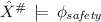. If the verification holds we have a solution, and exit the loop. Otherwise, we find a counterexample iteration k and corresponding initial point $x_0$ for which the property does not hold, which we use to locally refine the abstraction. When the abstraction cannot be further refined, we provide them to the abstract phase.

• 4. If we reach the abstract phase, it means that the candidate solution is not valid, in which case we must refine the abstraction used by the synthesizer.

  • (a) Find the constraints that invalidate the property as a set of counterexamples for the eigenvalues, which we define as $\phi _\Lambda$. This is a constraint in the spectrum i.e., transfer function) of the closed loop dynamics.

  • (b) We use $\phi _\Lambda$ to further constrain the characteristic polynomial $z^n+\sum _{i=1}^n(a_i-k_i)z^{n-i}=\prod _{i=1}^n (z-\lambda _i) : |\lambda _i|<1 \wedge \lambda _i \models \phi _{\Lambda }$. These constraints correspond to specific iterations for which the system may be unsafe.

  • (c) Pass the refined abstraction $\phi (K)$ with the new constraints and the list of iterations k to the synthesize phase.

Illustrative Example. Let us consider the following example with discretized dynamics

$$A_d = \left[ \begin{array}{ccc}2.6207&{}-1.1793&{}0.65705\\ 2&{}0&{}0\\ 0&{}0.5&{}0\end{array}\right] , \quad B_d = \left[ \begin{array}{c}8\\ 0\\ 0\end{array}\right] $$

Using the initial state bounds $\underline{x_{0}}=-0.9$ and $\overline{x_{0}}=0.9$, the input bounds $\underline{u}=-10$ and $\overline{u}=10$, and safety specifications $\underline{x_{i}}=-0.92$ and $\overline{x_{i}}=0.92$, the synthesize phase in Fig. 4 generates an initial candidate controller $K=[\begin{array}{ccc}0.24609375&-0.125&0.1484375\end{array}]$. This candidate is chosen for its closed-loop stable dynamics, but the verify phase finds it to be unsafe and returns a list of iterations with an initial state that fails the safety specification $(k,x_0) {\in } \{ (2, [\begin{array}{ccc}0.9&-0.9&0.9\end{array}]),(3, [\begin{array}{ccc}0.9&-0.9&-0.9\end{array}])\}$. This allows the abstract phase to create a new safety specification that considers these iterations for these initial states to constrain the solution space. This refinement allows synthesize to find a new controller $K=[\begin{array}{ccc}0.23828125&-0.17578125&0.109375\end{array}]$, which this time passes the verification phase, resulting in a safe system.

Fig. 4.

Abstraction-based CEGIS

5 Experimental Evaluation

5.1 Description of the Benchmarks

A set of state-space models for different classes of systems has been taken from the literature [1, 13, 23, 31] and employed for validating our methodology.

DC Motor Rate plants describes the angular velocity of a DC Motor, respectively. The Automotive Cruise System plant represents the speed of a motor vehicle. The Helicopter Longitudinal Motion plant provides the longitudinal motion model of a helicopter. The Inverted Pendulum plant describes a pendulum model with its center of mass above its pivot point. The Magnetic Suspension plant provides a physical model for which a given object is suspended via a magnetic field. The Magnetized Pointer plant describes a physical model employed in analogue gauges and indicators that is rotated through interaction with magnetic fields. The 1/4 Car Suspension plant presents a physical model that connects a car to its wheels and allows relative motion between the two parts. The Computer Tape Driver plant describes a system to read and write data on a storage device.

Our benchmarks are SISO models (Sect. 3). The Inverted Pendulum appears to be a two-output system, but it is treated as two SISO models during the experiments. All the state measurements are assumed to be available (current work targets the extension of our framework to observer-based synthesis).

All benchmarks are discretized with different sample times [11]. All experiments are performed considering $\underline{x_{i}}=-1$ and $\overline{x_{i}}=1$ and the reference inputs $r_{k}=0, \forall k>0$. We conduct the experimental evaluation on a 12-core 2.40 GHz Intel Xeon E5-2440 with 96 GB of RAM and Linux OS. We use the Linux times command to measure CPU time used for each benchmark. The runtime is limited to one hour per benchmark.

5.2 Objectives

Using the state-space models given in Sect. 5.1, our evaluation has the following two experimental goals:

• EG1 (CEGIS) Show that both the multi-staged and the abstraction-based CEGIS approaches are able to generate FWL digital controllers in a reasonable amount of time.

• EG2 (sanity check) Confirm the stability and safety of the synthesized controllers outside of our model.

5.3 Results

We provide the results in Table 1. Here Benchmark is the name of the respective benchmark, Order is the number of continuous variables, $\mathcal {F}_{\langle I_p,F_p \rangle }$ is the fixed-point precision used to model the plant, while Time is the total time required to synthesize a controller for the given plant with one of the two methods. Timeouts are indicated by ✗. The precision for the controller, $\mathcal {F}_{\langle I_c,F_c \rangle }$, is chosen to be $I_c = 8$, $F_c = 8$.

For the majority of our benchmarks, we observe that the abstraction-based back-end is faster than the basic multi-staged verification approach, and finds one solution more (9) than the multi-staged back-end (8). In direct comparison, the abstraction-based approach is on average able to find a solution in approximately 70% of the time required using the multi-staged back-end, and has a median run-time 1.4 s, which is seven times smaller than the multi-staged approach. The two back-ends complement each other in benchmark coverage and together solve all benchmarks in the set. On average our engine spent 52% in the synthesis and 48% in the verification phase.

Table 1. Experimental results.

The median run-time for our benchmark set is 9.4 s. Overall, the average synthesis time amounts to approximately 15.6 s. We consider these times short enough to be of practical use to control engineers, and thus affirm EG1.

There are a few instances for which the system fails to find a controller. For the naïve approach, the completeness threshold may be too large, thus causing a timeout. On the other hand, the abstraction-based approach may require a very precise abstraction, resulting in too many refinements and, consequently, in a timeout. Yet another source of incompleteness is the inability of the synthesize phase to use a large enough precision for the plant model.

The synthesized controllers are confirmed to be safe outside of our model representation using MATLAB, achieving EG2. A link to the full experimental environment, including scripts to reproduce the results, all benchmarks and the tool, is provided in the footnote as an Open Virtual Appliance (OVA).¹ The provided experimental environment runs multiple discretisations for each benchmark, and lists the fastest as the result synthesis time.

5.4 Threats to Validity

Benchmark Selection: We report an assessment of both our approaches over a diverse set of real-world benchmarks. Nevertheless, this set of benchmarks is limited within the scope of this paper and the performance may not generalize to other benchmarks.

Plant Precision and Discretization Heuristics: Our algorithm to select suitable FWL word widths to model the plant behavior increases the precision by 8 bits at each step in order to be compliant with the CBMC type API. Similarly, for discretization, we run multiple discretizations for each benchmark and retain the fastest run. This works sufficiently well for our benchmarks, but performance may suffer in some cases, for example if the completeness threshold is high.

Abstraction on Other Properties: The performance gain from abstract acceleration may not hold for more complex properties than safety, for instance “eventually reach and always remain in a given safe set”.

6 Conclusion

We have presented two automated approaches to synthesize digital state-feedback controllers that ensure both stability and safety over the state-space representation. The first approach relies on unfolding of the closed-loop model dynamics up to a completeness threshold, while the second one applies abstraction refinement and acceleration to increase speed whilst retaining soundness. Both approaches are novel within the control literature: they give a fully automated synthesis method that is algorithmically and numerically sound, considering various error sources in the implementation of the digital control algorithm and in the computational modeling of plant dynamics. Our experimental results show that both approaches are able to synthesize safe controllers for most benchmarks within a reasonable amount of time fully automatically. In particular, both approaches complement each other and together solve all benchmarks, which have been derived from the control literature.

Future work will focus the extension of these approaches to the continuous-time case, to models with output-based control architectures (with the use of observers), and to the consideration of more complex specifications.

Appendices

A Stability of Closed-Loop Models

1.1 A.1Stability of Closed-Loop Models with Fixed-Point Controller Error

The proof of Jury’s criterion [11] relies on the fact that the relationship between states and next states is defined by $x_{k+1} = (A_d - B_dK) x_k$, all computed at infinite precision. When we employ a FWL digital controller, the operation becomes:

$$\begin{aligned} x_{k+1}&= A_d \cdot x_{k} -(\mathcal {F}_{\langle I_c,F_c \rangle }(K)\cdot \mathcal {F}_{\langle I_c,F_c \rangle }(x_{k})). \\ x_{k+1}&= (A_d - B_dK) \cdot x_k + B_dK\delta , \end{aligned}$$

where $\delta$ is the maximum error that can be introduced by the FWL controller in one step, i.e., by reading the states values once and multiplying by K once. We derive the closed form expression for $x_n$ as follows:

$$\begin{aligned} x_{1}&= (A_d - B_dK)x_0 + B_dK\delta \\ x_{2}&=(A_d - B_dK)^2x_0 + (A_d - B_dK)B_dK\delta + B_dK\delta \\ x_{n}&= (A_d - B_dK)^nx_0 + (A_d - B_dK)^{n-1}B_dK\delta + ... + (A_d - B_dK)^1B_dK \delta + B_dK\delta \\&= (A_d - B_dK)^nx_0 + \sum _{i=0}^{i=n-1}(A_d - B_dK)^iB_dk\delta . \end{aligned}$$

The definition of asymptotic stability is that the system converges to a reference signal, in this case we use no reference signal so an asymptotically stable system will converge to the origin. We know that the original system with an infinite-precision controller is stable, because we have synthesized it to meet Jury’s criterion. Hence, $(A_d - B_dK)^n x_0$ must converge to zero.

The power series of matrices converges [15] iff the eigenvalues of the matrix are less than 1 as follows: $\sum _{i=0}^{\infty }T^i = (I - T)^{-1}$, where I is the identity matrix and T is a square matrix. Thus, our system will converge to the value

$$\begin{aligned} 0 + (I - A_d + B_dK)^{-1}B_dk\delta . \end{aligned}$$

As a result, if the value $(I - A_d + B_dK)^{-1}B_dk\delta$ is within the safe space, then the synthesized fixed-point controller results in a safe closed-loop model. The convergence to a finite value, however, will not make it asymptomatically stable.

B Errors in LTI Models

1.1 B.1 Errors Due to Numerical Representation

We have used $\mathcal {F}_{\langle I,F \rangle }(x)$ denote a real number x represented in a fixed point domain, with I bits representing the integer part and F bits representing the decimal part. The smallest number that can be represented in this domain is $c_m=2^{-F}$. The following approximation errors will arise in mathematical operations and representation:

• 1. Truncation: Let x be a real number, and $\mathcal {F}_{\langle I,F \rangle }(x)$ be the same number represented in a fixed-point domain as above. Then $\mathcal {F}_{\langle I,F \rangle }(x) = x-\delta _T$ where the error $\delta _T=x\ \%_{c_m}\ \tilde{x}$, and $\%_{c_m}$ is the modulus operation performed on the last bit. Thus, $\delta _T$ is the truncation error and it will propagate across operations.

• 2. Rounding: The following errors appear in basic operations. Let $c_1, c_2$ and $c_3$ be real numbers, and $\delta _{T1}$ and $\delta _{T2}$ be the truncation errors caused by representing $c_1$ and $c_2$ in the fixed-point domain as above.

  • (a) Addition/Subtraction: these operations only propagate errors coming from truncation of the operands, namely $\mathcal {F}_{\langle I,F \rangle }(c_1) \pm \mathcal {F}_{\langle I,F \rangle }(c_2) = c_3 + \delta _3$ with $|\delta _3| \le |\delta _{T1}| + |\delta _{T2}|$.

  • (b) Multiplication: $\mathcal {F}_{\langle I,F \rangle }(c_1) \cdot \mathcal {F}_{\langle I,F \rangle }(c_2) = c_3 + \delta _3$ with $|\delta _3| \le |\delta _{T1}\cdot \mathcal {F}_{\langle I,F \rangle }(c_2)|+ |\delta _{T2}\cdot \mathcal {F}_{\langle I,F \rangle }(c_1)| + c_m$, where $c_m=2^{-F}$ as above.

  • (c) Division: the operations performed by our controllers in the FWL domain do not include division. However, we do use division in computations at the precision of the plant. Here the error depends on whether the divisor is greater or smaller than the dividend: $\mathcal {F}_{\langle I,F \rangle }(c_1) / \mathcal {F}_{\langle I,F \rangle }(c_2) = c_3 + \delta _{T3}$ where $\delta _{T3}$ is $(\delta _{T2}\cdot c_1 - \delta _{T1}\cdot c_2)/(\delta _{T2}^2 - \delta _{T2} c_2)$,

• 3. Overflow: The maximum size of a real number x that can be represented in a fixed point domain as $\mathcal {F}_{\langle I,F \rangle }(x)$ is $\pm (2^{I-1}+1-2^{-F})$. Numbers outside this range cannot be represented by the domain. We check that overflow does not occur.

1.2 B.2 Modeling Quantization as Noise

During any given ADC conversion, the continuous signal will be sampled in the real domain and transformed by $\mathcal {F}\langle I_{c},F_{c} \rangle (x)$ (assuming the ADC discretization is the same as the digital implementation). This sampling uses a threshold which is defined by the less significant bit ($q_{c}=c_{m_c}=2^{-F_c}$) of the ADC and some non-linearities of the circuitry. The overall conversion is

$$\mathcal {F}\langle I_{c},F_{c} \rangle (y(t)) = y_k : y_k \in \left[ y(t)-\frac{q_{c}}{2}\ \ \ \ y(t)+\frac{q_{c}}{2}\right] .$$

If we denote the error in the conversion by $\nu _k=y_k-y(t)$ where $t = nk$, and n is the sampling time and k the number of steps, then we may define some bounds for it $\nu _k \in [-\frac{q_{c}}{2}\ \ \frac{q_{c}}{2}]$.

We will assume, for the purposes of this analysis, that the domain of the ADC is that of the digital controller (i.e., the quantizer includes any digital gain added in the code). The process of quantization in the DAC is similar except that it is calculating $\mathcal {F}\langle I_{dac},F_{dac} \rangle (\mathcal {F}\langle I_{c},F_{c} \rangle (x))$. If these domains are the same ($I_{c}=I_{dac},F_{c}=F_{dac}$), or if the DAC resolution in higher than the ADCs, then the DAC quantization error is equal to zero. From the above equations we can now define the ADC and DAC quantization noises ${\nu _1}_k \in [-\frac{q_1}{2}\ \ \frac{q_1}{2}]$ and ${\nu _2}_k \in [-\frac{q_2}{2}\ \ \frac{q_2}{2}]$, where $q_1=q_{c}$ and $q_2=q_ dac$. This is illustrated in Fig. 1 where $Q_1$ is the quantizer of the ADC and $Q_2$ the quantizer for the DAC. These bounds hold irrespective of whether the noise is correlated, hence we may use them to over-approximate the noise effect on the state space progression over time. The resulting dynamics are

$$\begin{aligned} {x}_{k+1} = {A}_d{x}_k+{B}_d({u}_k+{{\nu }_2}_k), \quad u_k = -K{x}_{k}+{{\nu }_1}_k, \end{aligned}$$

which result in the following closed-loop dynamics:

$$\begin{aligned} {x}_{k+1}&= ({A}_d-{B}_d{K}_d) {x}_k+{B}_d{{\nu }_2}_k +{{\nu }_1}_k. \end{aligned}$$

References

Control tutorials for MATLAB and SIMULINK. http://ctms.engin.umich.edu/
Abate, A., Bessa, I., Cattaruzza, D., Cordeiro, L.C., David, C., Kesseli, P., Kroening, D.: Sound and automated synthesis of digital stabilizing controllers for continuous plants. In: Hybrid Systems: Computation and Control (HSCC), pp. 197–206. ACM (2017)
Anta, A., Majumdar, R., Saha, I., Tabuada, P.: Automatic verification of control system implementations. In: EMSOFT, pp. 9–18 (2010)
Åström, K., Wittenmark, B.: Computer-Controlled Systems: Theory and Design. Prentice Hall Information and System Sciences Series. Prentice Hall, Upper Saddle River (1997)
Bessa, I., Ismail, H., Palhares, R., Cordeiro, L., Filho, J.E.C.: Formal non-fragile stability verification of digital control systems with uncertainty. IEEE Trans. Comput. 66(3), 545–552 (2017)
Brain, M., Tinelli, C., Rümmer, P., Wahl, T.: An automatable formal semantics for IEEE-754 floating-point arithmetic. In: ARITH, pp. 160–167. IEEE (2015)
Cattaruzza, D., Abate, A., Schrammel, P., Kroening, D.: Unbounded-time analysis of guarded LTI systems with inputs by abstract acceleration. In: Blazy, S., Jensen, T. (eds.) SAS 2015. LNCS, vol. 9291, pp. 312–331. Springer, Heidelberg (2015). doi:10.1007/978-3-662-48288-9_18
David, C., Kroening, D., Lewis, M.: Using program synthesis for program analysis. In: Davis, M., Fehnker, A., McIver, A., Voronkov, A. (eds.) LPAR 2015. LNCS, vol. 9450, pp. 483–498. Springer, Heidelberg (2015). doi:10.1007/978-3-662-48899-7_34
de Bessa, I.V., Ismail, H., Cordeiro, L.C., Filho, J.E.C.: Verification of fixed-point digital controllers using direct and delta forms realizations. Des. Autom. Emb. Syst. 20(2), 95–126 (2016)
Duggirala, P.S., Viswanathan, M.: Analyzing real time linear control systems using software verification. In: IEEE Real-Time Systems Symposium, pp. 216–226, December 2015
Fadali, S., Visioli, A.: Digital Control Engineering: Analysis and Design. Electronics & Electrical. Elsevier/Academic Press, Amsterdam/Cambridge (2009)
Fialho, I.J., Georgiou, T.T.: On stability and performance of sampled-data systems subject to wordlength constraint. IEEE Trans. Autom. Control 39(12), 2476–2481 (1994)
Franklin, G., Powell, D., Emami-Naeini, A.: Feedback Control of Dynamic Systems, 7th edn. Pearson, Upper Saddle River (2015)
Frehse, G., et al.: SpaceEx: scalable verification of hybrid systems. In: Gopalakrishnan, G., Qadeer, S. (eds.) CAV 2011. LNCS, vol. 6806, pp. 379–395. Springer, Heidelberg (2011). doi:10.1007/978-3-642-22110-1_30
Horn, R.A., Johnson, C.: Matrix Analysis. Cambridge University Press, Cambridge (1990)
Itzhaky, S., Gulwani, S., Immerman, N., Sagiv, M.: A simple inductive synthesis methodology and its applications. In: OOPSLA, pp. 36–46. ACM (2010)
Kroening, D., Strichman, O.: Efficient computation of recurrence diameters. In: Zuck, L.D., Attie, P.C., Cortesi, A., Mukhopadhyay, S. (eds.) VMCAI 2003. LNCS, vol. 2575, pp. 298–309. Springer, Heidelberg (2003). doi:10.1007/3-540-36384-X_24
Li, G.: On pole and zero sensitivity of linear systems. IEEE Trans. Circuits Syst.-I: Fundam. Theory Appl. 44(7), 583–590 (1997)
Liberzon, D.: Hybrid feedback stabilization of systems with quantized signals. Automatica 39(9), 1543–1554 (2003)
Liu, J., Ozay, N.: Finite abstractions with robustness margins for temporal logic-based control synthesis. Nonlinear Anal.: Hybrid Syst. 22, 1–15 (2016)
Mazo, M., Davitian, A., Tabuada, P.: PESSOA: a tool for embedded controller synthesis. In: Touili, T., Cook, B., Jackson, P. (eds.) CAV 2010. LNCS, vol. 6174, pp. 566–569. Springer, Heidelberg (2010). doi:10.1007/978-3-642-14295-6_49
Moore, R.E.: Interval Analysis, vol. 4. Prentice-Hall, Englewood Cliffs (1966)
Oliveira, V.A., Costa, E.F., Vargas, J.B.: Digital implementation of a magnetic suspension control system for laboratory experiments. IEEE Trans. Educ. 42(4), 315–322 (1999)
Oudjida, A.K., Chaillet, N., Liacha, A., Berrandjia, M.L., Hamerlain, M.: Design of high-speed and low-power finite-word-length PID controllers. Control Theory Technol. 12(1), 68–83 (2014)
Park, J., Pajic, M., Lee, I., Sokolsky, O.: Scalable verification of linear controller software. In: Chechik, M., Raskin, J.-F. (eds.) TACAS 2016. LNCS, vol. 9636, pp. 662–679. Springer, Heidelberg (2016). doi:10.1007/978-3-662-49674-9_43
Picasso, B., Bicchi, A.: Stabilization of LTI systems with quantized state - quantized input static feedback. In: Maler, O., Pnueli, A. (eds.) HSCC 2003. LNCS, vol. 2623, pp. 405–416. Springer, Heidelberg (2003). doi:10.1007/3-540-36580-X_30
Ravanbakhsh, H., Sankaranarayanan, S.: Counter-example guided synthesis of control Lyapunov functions for switched systems. In: Conference on Decision and Control (CDC), pp. 4232–4239 (2015)
Ravanbakhsh, H., Sankaranarayanan, S.: Robust controller synthesis of switched systems using counterexample guided framework. In: EMSOFT, pp. 8:1–8:10. ACM (2016)
Roux, P., Jobredeaux, R., Garoche, P.: Closed loop analysis of control command software. In: HSCC, pp. 108–117. ACM (2015)
Solar-Lezama, A., Tancau, L., Bodík, R., Seshia, S.A., Saraswat, V.A.: Combinatorial sketching for finite programs. In: ASPLOS, pp. 404–415. ACM (2006)
Tan, R.H.G., Hoo, L.Y.H.: DC-DC converter modeling and simulation using state space approach. In: IEEE Conference on Energy Conversion, CENCON, pp. 42–47, October 2015
Wang, T.E., Garoche, P., Roux, P., Jobredeaux, R., Feron, E.: Formal analysis of robustness at model and code level. In: HSCC, pp. 125–134. ACM (2016)
Wu, J., Li, G., Chen, S., Chu, J.: Robust finite word length controller design. Automatica 45(12), 2850–2856 (2009)
Zamani, M., Mazo, M., Abate, A.: Finite abstractions of networked control systems. In: IEEE CDC, pp. 95–100 (2014)
Author information
Authors and Affiliations
Corresponding author
Editor information
Editors and Affiliations