Working with Type-2 Fuzzy Sets

Abstract

This chapter explains how to work with type-2 fuzzy sets (T2 FSs). Most of its topics are needed in the rest of this book. Coverage includes: set-theoretic operations (union, intersection, and complement) for general type-2 fuzzy sets (GT2 FSs) computed using the Extension Principle , set-theoretic operations for interval type-2 fuzzy sets (IT2 FSs), set-theoretic operations for GT2 FSs computed using horizontal slices , type-2 relations and compositions on the same product space and on different product spaces , compositions of a T2 FS with a type-2 relation, type-2 hedges, Extension Principle for IT2 and GT2 FSs , functions of GT2 FSs computed using $\alpha$-planes, Cartesian product of T2 FSs, implications , an appendix about the properties of T2 FSs and an appendix that has detailed proofs of many theorems. 27 examples are used to illustrate the chapter’s important concepts.

Appendices

Appendix 1: Properties of T2 FSs

This appendix is analogous to Appendix 1 in Chap. 2. It presents details about properties/laws of T2 FSs and, as in that Chap. 2 appendix, examines the following frequently used laws to see if they remain satisfied under maximum t-conorm and either minimum or product t-norms¹⁷:

Reflexive, anti-symmetric, transitive, idempotent, commutative, associative, absorption, distributive, involution, De Morgan’s, and identity

Recall, again, that the reason for doing this is that rules in a rule-based system may make use of the words “and”, “or”, “unless”, “not”, etc., but all of the mathematics for such a system is worked out in this book only for canonical rules that use the words “and” and “or”. Section 3.2 showed how the former rules are transformed into the canonical rules by using some of the above laws. So, it is important to know when or if the use of these laws is correct when rules use T2 FSs.

Because the union and intersection of T2 FSs require computing the join and meet of the secondary MFs of these sets, set-theoretic laws for T2 FSs can be expressed in terms of secondary MFs.

Tables 7.1 and 7.2 are the type-2 counterparts to Table 2.8. Table 7.1 is for the minimum t-norm, whereas Table 7.2 is for the product t-norm. What complicates the study of the above laws for GT2 FSs is that their secondary MFs may in general be: normal and convex, or non-normal and convex, or normal and non-convex, or non-normal and non-convex, which is why Tables 7.1 and 7.2 have four columns with those headings.

For the product t-norm there can be two different situations, namely: (1) $\star = {\text{product}}$ and $\wedge = {\text{product}}$, and (2) $\star = {\text{product}}$ and $\wedge = {\text{minimum}}$. Only Situation 1 is considered in this book because it seems more consistent to this author to choose both $\star$ and $\wedge$ to be the same. Situation 2 was introduced in Mizumoto and Tanaka (1976) and set-theoretic properties for it can be found in that reference.

Table 7.1 Summary of set-theoretic laws and whether or not they are satisfied for GT2 FSs under maximum t-conorm and minimum t-norm^a

Table 7.2 Summary of set-theoretic laws and whether or not they are satisfied for GT2 FSs under maximum t-conorm and product t-norm^a

The secondary MFs for an IT2 FS are type-1 interval fuzzy numbers , and so they are normal and convex. Consequently for IT2 FSs, one only needs to examine the “Normal/Convex” columns of Tables 7.1 and 7.2. All of the above laws/properties that are satisfied for T1 FSs for minimum and product t-norms are also satisfied for IT2 FSs (see Exercises 7.37 and 7.38).

Observe, from Tables 7.1 and 7.2, that:

• For the minimum t-norm (Table 7.1), all laws are satisfied for normal and convex secondary MFs; this provides a very strong reason for using such secondary MFs.

• For the product t-norm (Table 7.2), the most number of laws (but not all of the laws) satisfied are for normal and convex secondary MFs, which again provides a very strong reason for using such secondary MFs.

• If a law is violated for normal and convex secondary MFs (Table 7.2) it is violated for the three other kinds of secondary MFs; however, if a law is not violated for normal and convex secondary MFs (Tables 7.1 and 7.2), it may or may not be violated for the three other kinds of secondary MFs.

Recall that all operations on GT2 FSs sets collapse to their type-1 counterparts when each secondary MF is replaced by its support at which the secondary grades are equal to 1. For simplicity, it is assumed here that the secondary MFs reach the value 1 at only one point. As explained in Sect. 6.8, this means that a T1 FS can be thought of as a special case of a GT2 FS; i.e., the case where only one value of the secondary MF has a secondary grade equal to 1 and all other secondary grades are equal to zero. Consequently, if there are any set-theoretic laws that are not satisfied by T1 FSs it can safely be said that T2 FSs will not satisfy those laws either; however, the converse of this statement may not be true. If any condition is satisfied by T1 FSs, it may or may not be satisfied by GT2 FSs.

This could be a very long appendix if it provided the details for all of the 20 laws (some have two or even four versions), four kinds of secondary MFs and two t-norms (a total of 160 calculations). Most of this is left as exercises for the reader. Below some of the details are given but only for the product t-norm and normal and convex secondary MFs (Table 7.2).

Consider three T2 FSs, $\tilde{A},\,\tilde{B},\,{\text{and}}\,\tilde{C}$ defined on the same universe of discourse, $X$, with secondary MFs as follows, for $x \in X$:

$$ \mu_{{\tilde{A}(x)}} (u) = \int\limits_{u \in [0,1]} {f_{x} (u)/u} $$

(7.116)

$$ \mu_{{\tilde{B}(x)}} (u) = \int\limits_{u \in [0,1]} {g_{x} (u)/u} $$

(7.117)

$$ \mu_{{\tilde{C}(x)}} (u) = \int\limits_{u \in [0,1]} {h_{x} (u)/u} $$

(7.118)

To begin, our attention is directed at the laws that are satisfied. As in Klir and Yuan (1995), fuzzy set inclusion is defined to mean:

$$ \tilde{A} \subseteq \tilde{B} \Leftrightarrow \mu_{{\tilde{A}(x)}} \le \mu_{{\tilde{B}(x)}}\quad x \in X $$

(7.119)

Since this does not make use of the t-norm or t-conorm, it is satisfied. The generalized versions of reflexive, anti-symmetric, and transitive laws, as stated in Tables 7.1 and 7.2, are also satisfied because they do not make use of the t-norm or t-conorm. Note that, in these laws, $\mu_{{\tilde{A}(x)}} = \mu_{{\tilde{B}(x)}} \Leftrightarrow f_{x} (u) = g_{x} (u)$, $u \in [0,1]$.

Commutative laws are satisfied for maximum t-conorm and product t-norm (Mizumoto and Tanaka 1976), e.g., using (7.3):

$$ \begin{aligned} \mu_{{\tilde{A}(x)}} \sqcup \mu_{{\tilde{B}(x)}} & = \left[ {\int\limits_{u \in [0,1]} {f_{x} (u)/u} } \right] \sqcup \left[ {\int\limits_{v \in [0,1]} {g_{x} (v)/v} } \right] \\ & = \int\limits_{u \in [0,1]} {\int\limits_{v \in [0,1]} {f_{x} (u) \times g_{x} (v)/(u \vee v)} } = \int\limits_{u \in [0,1]} {\int\limits_{v \in [0,1]} {g_{x} (v) \times f_{x} (u)/(v \vee u)} } \\ & = \left[ {\int\limits_{v \in [0,1]} {g_{x} (v)/v} } \right] \sqcup \left[ {\int\limits_{u \in [0,1]} {f_{x} (u)/u} } \right] = \mu_{{\tilde{B}(x)}} \sqcup \mu_{{\tilde{A}(x)}} \\ \end{aligned} $$

(7.120)

Associative laws are also satisfied for maximum t-conorm and product t-norm (Mizumoto and Tanaka 1976), e.g., using (7.7):

$$ \begin{aligned} \mu_{{\tilde{A}(x)}} \sqcap \left( {\mu_{{\tilde{B}(x)}} \sqcap \mu_{{\tilde{C}(x)}} } \right) & = \left[ {\int\limits_{u \in [0,1]} {f_{x} (u)/u} } \right]\sqcap \left[ {\int\limits_{v \in [0,1]} {\int\limits_{w \in [0,1]} {g_{x} (v) \times h_{x} (w)/(v \times w)} } } \right] \\ & = \int\limits_{u \in [0,1]} {\int\limits_{v \in [0,1]} {\int\limits_{w \in [0,1]} {f_{x} (u) \times [g_{x} (v) \times h_{x} (w)]/u \times (v \times w)} } } \\ & = \int\limits_{u \in [0,1]} {\int\limits_{v \in [0,1]} {\int\limits_{w \in [0,1]} {[f_{x} (u) \times g_{x} (v)] \times h_{x} (w)/(u \times v) \times w} } } \\ & = \left[ {\int\limits_{u \in [0,1]} {\int\limits_{v \in [0,1]} {f_{x} (u) \times g_{x} (v)/(u \times v)} } } \right]\sqcap \left[ {\int\limits_{w \in [0,1]} {h_{x} (w)/w} } \right] \\ & = \left( {\mu_{{\tilde{A}(x)}} \sqcap \mu_{{\tilde{B}(x)}} } \right)\sqcap \mu_{{\tilde{C}(x)}} \\ \end{aligned} $$

(7.121)

The identity laws are all satisfied for maximum t-conorm and product t-norm if one uses normal membership grades, because:

$$ \begin{aligned} \mu_{{\tilde{A}(x)}} \sqcup (1/0) & = \left[ {\int\limits_{u \in [0,1]} {f_{x} (u)/u} } \right] \sqcup 1/0 \\ & = \int\limits_{u \in [0,1]} {f_{x} (u) \times 1/(u \vee 0) = \int\limits_{u \in [0,1]} {f_{x} (u)/u} = } \,\,\mu_{{\tilde{A}(x)}} \\ \end{aligned} $$

(7.122)

$$ \begin{aligned} \mu_{{\tilde{A}(x)}} \sqcap (1/1) & = \left[ {\int\limits_{u \in [0,1]} {f_{x} (u)/u} } \right]\sqcap 1/1 \\ & = \int\limits_{u \in [0,1]} {f_{x} (u) \times 1/(u \times 1) = \int\limits_{u \in [0,1]} {f_{x} (u)/u} = } \,\,\mu_{{\tilde{A}(x)}} \\ \end{aligned} $$

(7.123)

$$ \begin{aligned} \mu_{{\tilde{A}(x)}} \sqcup (1/1) & = \left[ {\int\limits_{u \in [0,1]} {f_{x} (u)/u} } \right] \sqcup 1/1 = \int\limits_{u \in [0,1]} {f_{x} (u) \times 1/(u \vee 1)} \\ & = \int\limits_{u \in [0,1]} {f_{x} (u)/1} = \left[ {\mathop {\sup }\limits_{u} f_{x} (u)} \right]/1 = 1/1 \\ \end{aligned} $$

(7.124)

$$ \begin{aligned} \mu_{{\tilde{A}(x)}} \sqcap (1/0) & = \left[ {\int\limits_{u \in [0,1]} {f_{x} (u)/u} } \right]\sqcap 1/0 = \int\limits_{u \in [0,1]} {f_{x} (u) \times 1/(u \times 0)} \\ & = \int\limits_{u \in [0,1]} {f_{x} (u)/0} = \left[ {\mathop {\sup }\limits_{u} f_{x} (u)} \right]/0 = 1/0 \\ \end{aligned} $$

(7.125)

The fact that the secondary MFs are normal only had to be used in (7.124) and (7.125). It was not used in the proofs of (7.122) and (7.123); hence, those identity laws hold even in the case of non-normal secondary MFs. Convexity of $\mu_{{\tilde{A}(x)}}$ played no role in these calculations.

Next, out attention is directed at the laws that are not satisfied. Examining (7.124) and (7.125), these laws fail when $\tilde{A}(x)$ is non-normal. The following counterexample demonstrates that the first parts of the idempotent and distributive laws, and the second part of the absorption law, which are satisfied in the type-1 case, are not satisfied for maximum t-conorm and product t-norm in the type-2 case.

Example 7.27

Consider the following three normal convex type-1 secondary MFs:

$$ \mu_{{\tilde{A}(x)}} (u) = 0.5/0.1 + 1/0.7 $$

(7.126)

$$ \mu_{{\tilde{B}(x)}} (u) = 0.6/0.3 + 1/0.7 $$

(7.127)

$$ \mu_{{\tilde{C}(x)}} (u) = 0.4/0.2 + 1/0.8 $$

(7.128)

• Failure of the first part of the idempotent law under product t-norm:

  $$ \begin{aligned} \mu_{{\tilde{A}(x)}} \sqcup \mu_{{\tilde{A}(x)}} & = (0.5/0.1 + 1/0.7) \sqcup (0.5/0.1 + 1/0.7) \\ & = 0.25/0.1 + 0.5/0.7 + 0.5/0.7 + 1/0.7\\ & = 0.25/0.1 + 1/0.7 \ne \mu_{{\tilde{A}(x)}} \\ \end{aligned} $$

  (7.129)

• Failure of the first part of the distributive law under product t-norm (details are left to the reader in Exercise 7.44):

  $$ \begin{aligned} \mu_{{\tilde{A}(x)}} \sqcap (\mu_{{\tilde{B}(x)}} \sqcup \mu_{{\tilde{C}(x)}} ) & = 0.12/0.03 + 0.2/0.07 + 0.5/0.08 \\ & \quad + 0.24/0.21 + 0.4/0.49 + 1/0.56 \\ \end{aligned} $$

  (7.130)
  $$ \begin{aligned} (\mu_{{\tilde{A}(x)}} \sqcap \mu_{{\tilde{B}(x)}} ) \sqcup (\mu_{{\tilde{A}(x)}} \sqcap \mu_{{\tilde{C}(x)}} ) & = 0.06/0.03 + 0.1/0.07 + 0.25/0.08 \\ & \quad + 0.2/0.14 + 0.3/0.21 + 0.5/0.49 + 1/0.56 \\ \end{aligned} $$

  (7.131)

Comparing (7.130) and (7.131), one concludes that $(\mu_{{\tilde{A}(x)}} \sqcap \mu_{{\tilde{B}(x)}} ) \sqcup (\mu_{{\tilde{A}(x)}} \sqcap \mu_{{\tilde{C}(x)}} ) \ne \mu_{{\tilde{A}(x)}} \sqcap (\mu_{{\tilde{B}(x)}} \sqcup \mu_{{\tilde{C}(x)}} )$.

• Failure of the second part of the absorption law under product t-norm (details are left to the reader in Exercise 7.44):

$$ \mu_{{\tilde{A}(x)}} \sqcup (\mu_{{\tilde{A}(x)}} \sqcap \mu_{{\tilde{B}(x)}} ) = 0.25/0.1 + 0.3/0.21 + 0.5/0.49 + 1/0.7 \ne \mu_{{\tilde{A}(x)}} $$

(7.132)

Observe from Table 7.2 that both of the distributive and absorption laws do not hold. So, under maximum t-conorm and product t-norm, meet is totally non-distributive and nonabsorptive for all GT2 FSs.

Appendix 2: Proofs

7.1.1 2.1 Proof of Theorem 7.1

The union of $\tilde{A}$ and $\tilde{B}$ is another GT2 FS, just as the union of T1 FSs A and B is another T1 FS; hence, using the vertical-slice representation of a GT2 FS in (6.38) and (6.39) applied to $\tilde{A} \cup \tilde{B}$, it follows that:

$$ \tilde{A} \cup \tilde{B} = \int\limits_{x \in X} {{{\mu_{{(\tilde{A} \cup \tilde{B})_{x} }} (u)} \mathord{\left/ {\vphantom {{\mu_{{(\tilde{A} \cup \tilde{B})_{x} }} (u)} x}} \right. \kern-0pt} x}} $$

(7.133)

where

$$ \mu_{{(\tilde{A} \cup \tilde{B})_{x} }} (u) = \int\limits_{u \in [0,1]} {{{h_{x} (u)} \mathord{\left/ {\vphantom {{h_{x} (u)} u}} \right. \kern-0pt} u}} $$

(7.134)

In (7.134), making use of (7.1) and (7.2),

$$ \int\limits_{u \in [0,1]} {{{h_{x} (u)} \mathord{\left/ {\vphantom {{h_{x} (u)} u}} \right. \kern-0pt} u}} = \varphi \left( {\mu_{{\tilde{A}(x)}} ,\mu_{{\tilde{B}(x)}} } \right) = \varphi \left( {\int\limits_{v \in [0,1]} {{{f_{x} (v)} \mathord{\left/ {\vphantom {{f_{x} (v)} v}} \right. \kern-0pt} v}} ,\int\limits_{w \in [0,1]} {{{g_{x} (w)} \mathord{\left/ {\vphantom {{g_{x} (w)} w}} \right. \kern-0pt} w}} } \right) $$

(7.135)

Applying (2.71) to the right-hand side of (7.135), it follows that:

$$ \varphi \left( {\int\limits_{v \in [0,1]} {{{f_{x} (v)} \mathord{\left/ {\vphantom {{f_{x} (v)} v}} \right. \kern-0pt} v}} ,\int\limits_{w \in [0,1]} {{{g_{x} (w)} \mathord{\left/ {\vphantom {{g_{x} (w)} w}} \right. \kern-0pt} w}} } \right) = \int\limits_{v \in [0,1]} {\int\limits_{w \in [0,1]} {{{f_{x} (v)\star g_{x} (w)} \mathord{\left/ {\vphantom {{f_{x} (v)\star g_{x} (w)} {\varphi (v,w)}}} \right. \kern-0pt} {\varphi (v,w)}}} } $$

(7.136)

where $\varphi$ is a t-conorm, chosen here as the maximum operation $\vee$, so that, from (7.134) to (7.136), it follows that:

$$ \mu_{{(\tilde{A} \cup \tilde{B})_{x} }} (u) = \int\limits_{u \in [0,1]} {{{h_{x} (u)} \mathord{\left/ {\vphantom {{h_{x} (u)} u}} \right. \kern-0pt} u}} = \int\limits_{v \in [0,1]} {\int\limits_{w \in [0,1]} {{{f_{x} (v)\star g_{x} (w)} \mathord{\left/ {\vphantom {{f_{x} (v)\star g_{x} (w)} {(\underbrace {v \vee w}_{u})}}} \right. \kern-0pt} {(\underbrace {v \vee w}_{u})}}} } \quad x \in X $$

(7.137)

In this equation $\iint {}$ indicates union over $[0,1] \times [0,1]$.

Applying (7.137) to (7.133), the result in (7.3) follows.

7.1.2 2.2 Proof of Theorem 7.3

• (a) Using (7.3) $F_{1} \sqcup F_{2}$ can be expressed as:

$$ F_{1} \sqcup F_{2} = \int\limits_{v \in [0,1]} {\int\limits_{w \in [0,1]} {{{[f_{1} (v)\star f_{2} (w)} \mathord{\left/ {\vphantom {{[f_{1} (v)\star f_{2} (w)} {(\theta = v \vee w}}} \right. \kern-0pt} {(\theta = v \vee w}}} } ) $$

(7.138)

If $\theta \in F_{1} \sqcup F_{2}$, the possible $\{ v,w\}$ pairs that can give $\theta$ as the result of the maximum operation are $\{ v,\theta \}$ where $v \in ( - \infty ,\theta ]$ and $\{ \theta ,w\}$ where $w \in ( - \infty ,\theta ]$. The process of finding the membership of $\theta$ in $F_{1} \sqcup F_{2}$ can be broken into three steps: (1) find the t-norm (minimum or product) between the memberships of all the pairs $\{ v,\theta \}$ such that $v \in ( - \infty ,\theta ]$ and then find their supremum; (2) do the same with all the pairs $\{ \theta ,w\}$ such that $w \in ( - \infty ,\theta ]$; and (3) find the maximum of the two suprema, i.e.

$$ \mu_{{F_{1} \sqcup F_{2} }} (\theta ) = \phi_{1} (\theta ) \vee \phi_{2} (\theta ) $$

(7.139)

where

$$ \phi_{1} (\theta ) = \mathop {\sup }\limits_{v \in ( - \infty ,\theta ]} \{ f_{1} (v)\star f_{2} (\theta )\} = f_{2} (\theta )\star \mathop {\sup }\limits_{v \in ( - \infty ,\theta ]} f_{1} (v) $$

(7.140)

and

$$ \phi_{2} (\theta ) = \mathop {\sup }\limits_{w \in ( - \infty ,\theta ]} \{ f_{1} (\theta )\star f_{2} (w)\} = f_{1} (\theta )\star \mathop {\sup }\limits_{w \in ( - \infty ,\theta ]} f_{2} (w) $$

(7.141)

To continue, $\theta$ is broken into the following three ranges: $\theta < {\xi}_{1}$, $\xi_{1} \le \theta < \xi_{2}$ and $\theta \ge \xi_{2}$ (see Fig. 7.17a). From the normality of $F_{i}$ $(i = 1,2)$, $f_{i} (\xi_{i} ) = 1$, and, from the convexity of $F_{i}$, $f_{i}$ is monotonic nondecreasing in $( - \infty ,\xi_{i} ]$ and monotonic nonincreasing in $[\xi_{i} ,\infty )$.

Fig. 7.17

a An example of $F_{1}$ and $F_{2}$ used in the proof of Part (a) of Theorem 7.3 [adapted from Fig. 6a in Karnik and Mendel (2001)]; and b $\mu_{{F_{1}\sqcup F_{2} }} (\theta )$ using the minimum t-norm

• (i) $\theta < \xi_{1}$: See Fig. 7.17a, where $\theta$ is called $\theta_{1}$. Because $f_{1}$ and $f_{2}$ both are monotonic nondecreasing in $( - \infty ,\xi_{1} ]$, $\sup_{v \in ( - \infty ,\theta ]} f_{1} (v) = f_{1} (\theta )$ and $\sup_{w \in ( - \infty ,\theta ]} f_{2} (w) = f_{2} (\theta )$; therefore, from (7.140) and (7.141), it follows that $\phi_{1} (\theta ) = \phi_{2} (\theta ) = f_{1} (\theta )\star f_{2} (\theta )$, so that:

$$ \mu_{{F_{1} \sqcup F_{2} }} (\theta ) = f_{1} (\theta )\star f_{2} (\theta ),\theta < \xi_{1} $$

(7.142)

• (ii) $\xi_{1} \le \theta < \xi_{2}$: See Fig. 7.17a, where $\theta$ is called $\theta_{2}$. Because $f_{1} (\xi_{1} ) = 1$ and $f_{2}$ is monotonic nondecreasing in $( - \infty ,\xi_{2} ]$, $\sup_{v \in ( - \infty ,\theta ]} f_{1} (v) = 1$ and $\sup_{w \in ( - \infty ,\theta ]} f_{2} (w) = f_{2} (\theta )$. Using these facts in (7.139)–(7.141), it follows that¹⁸:

$$ \mu_{{F_{1} \sqcup F_{2} }} (\theta ) = f_{2} (\theta ) \vee [f_{1} (\theta ) \wedge f_{2} (\theta )] = f_{2} (\theta ),\xi_{1} \le \theta < \xi_{2} $$

(7.143)

• (iii) $\theta \ge \xi_{2}$: See Fig. 7.17a, where $\theta$ is called $\theta_{3}$. For $\theta$ in this range, both $f_{1}$ and $f_{2}$ have already attained their maximum values; therefore $\sup_{v \in ( - \infty ,\theta ]} f_{1} (v) = \sup_{w \in ( - \infty ,\theta ]} f_{2} (w) = 1$. Consequently, from (7.139) to (7.141), it follows that:

$$ \mu_{{F_{1} \sqcup F_{2} }} (\theta ) = f_{1} (\theta ) \vee f_{2} (\theta ),\theta \ge \xi_{2} $$

(7.144)

Collecting (7.142)–(7.144) together, $\mu_{{F_{1} \sqcup F_{2} }} (\theta )$ can be expressed, as:

$$ \mu_{{F_{1} \sqcup F_{2} }} (\theta ) = \left\{ {\begin{array}{*{20}l} {f_{1} (\theta )\star f_{2} (\theta ),} & {\theta < \xi_{1} } \\ {f_{2} (\theta ),} & {\xi_{1} \le \theta < \xi_{2} } \\ {f_{1} (\theta ) \vee f_{2} (\theta ),} & {\theta \ge \xi_{2} } \\ \end{array} } \right. $$

(7.145)

which is (7.5).

Because both $F_{1}$ and $F_{2}$ are convex and normal, $F_{1} \sqcup F_{2}$ is convex and normal, via Theorem 7.2. It is also true that $\mu_{{F_{1} \sqcup F_{2} }} (\xi_{2} ) = 1$ (see Fig. 7.17b).

• (b) To prove (7.6), begin with $n = 3$, use the associative law for three T1 FSs (namely, $F_{1} \sqcup F_{2} \sqcup F_{3} = (F_{1} \sqcup F_{2} ) \sqcup F_{3}$), the fact that $F_{1} \sqcup F_{2}$ is convex and normal with $\mu_{{F_{1} \sqcup F_{2} }} (\xi_{2} ) = 1$, and the given facts that $f_{3} (\xi_{3} ) = 1$ and $\xi_{3} \ge \xi_{2}$, so that (7.145) can be directly applied to compute $\mu_{{(F_{1} \sqcup F_{2} ) \sqcup F_{3} }} (\theta )$, as:

$$ \mu_{{F_{1} \sqcup F_{2} \sqcup F_{3} }} (\theta ) = \left\{ {\begin{array}{*{20}l} {\mu_{{F_{1} \sqcup F_{2} }} (\theta )\star f_{3} (\theta ),} & {\theta < \xi_{2} } \\ {f_{3} (\theta ),} & {\xi_{2} \le \theta < \xi_{3} } \\ {\mu_{{F_{1} \sqcup F_{2} }} (\theta ) \vee f_{3} (\theta ),} & {\theta \ge \xi_{3} } \\ \end{array} } \right. $$

(7.146)

Because $\xi_{2} \le \xi_{3}$, (7.145) and (7.146) can be rewritten as:

$$ \mu_{{F_{1} \sqcup F_{2} }} (\theta ) = \left\{ {\begin{array}{*{20}l} {f_{1} (\theta )\star f_{2} (\theta ),} & {\theta < \xi_{1} } \\ {f_{2} (\theta ),} & {\xi_{1} \le \theta < \xi_{2} } \\ {f_{1} (\theta ) \vee f_{2} (\theta ),} & {\xi_{2} \le \theta < \xi_{3} } \\ {f_{1} (\theta ) \vee f_{2} (\theta ),} & {\theta \ge \xi_{3} } \\ \end{array} } \right. $$

(7.147)

$$ \mu_{{F_{1} \sqcup F_{2} \sqcup F_{3} }} (\theta ) = \left\{ {\begin{array}{*{20}l} {\mu_{{F_{1} \sqcup F_{2} }} (\theta )\star f_{3} (\theta ),} & {\theta < \xi_{1} } \\ {\mu_{{F_{1} \sqcup F_{2} }} (\theta )\star f_{3} (\theta ),} & {\xi_{1} \le \theta < \xi_{2} } \\ {f_{3} (\theta ),} & {\xi_{2} \le \theta < \xi_{3} } \\ {\mu_{{F_{1} \sqcup F_{2} }} (\theta ) \vee f_{3} (\theta ),} & {\theta \ge \xi_{3} } \\ \end{array} } \right. $$

(7.148)

Substituting for $\mu_{{F_{1} \sqcup F_{2} }} (\theta )$ from (7.147) into (7.148), it follows that:

$$ \mu_{{F_{1} \sqcup F_{2} \sqcup F_{3} }} (\theta ) = \left\{ {\begin{array}{*{20}l} {f_{1} (\theta )\star f_{2} (\theta )\star f_{3} (\theta ),} & {\theta < \xi_{1} } \\ {f_{2} (\theta )\star f_{3} (\theta ),} & {\xi_{1} \le \theta < \xi_{2} } \\ {f_{3} (\theta ),} & {\xi_{2} \le \theta < \xi_{3} } \\ {f_{1} (\theta ) \vee f_{2} (\theta ) \vee f_{3} (\theta ),} & {\theta \ge \xi_{3} } \\ \end{array} } \right. $$

(7.149)

(7.149) can be reexpressed as:

$$ \mu_{{F_{1} \sqcup F_{2} \sqcup F_{3} }} (\theta ) = \left\{ {\begin{array}{*{20}l} {T_{i = 1}^{3} f_{i} (\theta ),} & {\theta < \xi_{1} } \\ {T_{i = k + 1}^{3} f_{i} (\theta ),} & {\xi_{k} \le \theta < \xi_{k + 1} ,\,1 \le k \le 2} \\ { \vee_{i = 1}^{3} f_{i} (\theta ),} & {\theta \ge \xi_{3} } \\ \end{array} } \right. $$

(7.150)

(7.150) is the same as (7.6) for $n = 3$.

It is straightforward to show that $F_{1} \sqcup F_{2} \sqcup F_{3}$ is also a convex and normal T1 FS with $\mu_{{F_{1} \sqcup F_{2} \sqcup F_{3} }} (\xi_{3} ) = 1$; therefore, (7.145) can be applied again to obtain $\mu_{{F_{1} \sqcup F_{2} \sqcup F_{3} \sqcup F_{4} }}$. Continuing in this fashion (7.6) is obtained for all values of n.

7.1.3 2.3 Proof of Theorem 7.4

The intersection of $\tilde{A}$ and $\tilde{B}$ is another GT2 FS, just as the intersection of T1 FSs A and B is another T1 FS (Karnik and Mendel 2001, p. 343); hence, again using the vertical-slice representation of a GT2 FS in (6.38) and (6.39) applied to $\tilde{A} \cap \tilde{B}$, it follows that

$$ \tilde{A} \cap \tilde{B} = \int\limits_{x \in X} {{{\mu_{{(\tilde{A} \cap \tilde{B})_{x} }} (u)} \mathord{\left/ {\vphantom {{\mu_{{(\tilde{A} \cap \tilde{B})_{x} }} (u)} x}} \right. \kern-0pt} x}} $$

(7.151)

where

$$ \mu_{{(\tilde{A} \cap \tilde{B})_{x} }} (u) = \int\limits_{u \in [0,1]} {{{h_{x} (u)} \mathord{\left/ {\vphantom {{h_{x} (u)} u}} \right. \kern-0pt} u}} $$

(7.152)

Because the development of $\mu_{{(\tilde{A} \cap \tilde{B})_{x} }}$ is the same as the development of $\mu_{{(\tilde{A} \cup \tilde{B})_{x} }}$, except that in the present case $\varphi$ is the minimum or product function (again, corresponding to the type-1 case), namely $\wedge$, the rest of this proof is left to the reader (Exercise 7.6).

7.1.4 2.4 Proof of Theorem 7.6

For the case $n = 2$, $F_{1} \sqcap F_{2}$ can be expressed as (Karnik and Mendel 2001, p. 343):

$$ F_{1} \sqcap F_{2} = \int\limits_{v \in [0,1]} {\int\limits_{w \in [0,1]} {{{[f_{1} (v) \wedge f_{2} (w)} \mathord{\left/ {\vphantom {{[f_{1} (v) \wedge f_{2} (w)} {(\theta = v \wedge w}}} \right. \kern-0pt} {(\theta = v \wedge w}}} } ) $$

(7.153)

The only difference between this operation and the join operation in (7.138) is that $\theta \in F_{1} \sqcap F_{2}$ is the result of the minimum operation on some pair $\{ v,w\}$, such that $v \in F_{1}$ and $w \in F_{2}$; the possible such pairs being $\{ v,\theta \}$ where $v \in [\theta ,\infty )$ and $\{ \theta ,w\}$ where $w \in [\theta ,\infty )$. The process of finding the membership of $\theta$ in $F_{1} \sqcap F_{2}$ can be broken into three steps: (1) find the minima between the memberships of all the pairs $\{ v,\theta \}$ such that $v \in [\theta ,\infty )$ and then find their supremum; (2) do the same with all pairs $\{ \theta ,w\}$ such that $w \in [\theta ,\infty )$; and, (3) find the maximum of the two suprema.

Because the rest of the proof is very similar to the proof of Theorem 7.3, it is left to the reader (Exercise 7.7).

7.1.5 2.5 Proof of Theorem 7.7

By a type-2 fuzzy singleton (see Definition 6.26), is meant a T2 FS whose MF $\mu_{{\tilde{A}}} (x,v)$ is

$$ \mu_{{\tilde{A}}} (x,v) = \left\{ {\begin{array}{*{20}l} {1/1} & {x = x^{\prime}} \\ {1/0} & {\forall x \ne x^{\prime}} \\ \end{array} } \right. $$

(7.154)

Type-2 fuzzy set $\tilde{B}$ is described by (7.2). From (7.7), (7.154) and (7.2), and the last rows of Tables 7.1 and 7.2, it follows that, for minimum or product t-norms (for both of which $1\star g_{{x^{\prime}}} (w) = g_{{x^{\prime}}} (w)$ and $1 \wedge w = w$),

$$ \begin{aligned} \mu_{{\tilde{A}(x)}} \sqcap \mu_{{\tilde{B}(x)}} & = \left\{ {\begin{array}{*{20}l} {(1/1)\sqcap \tilde{B}(x^{\prime})} & {x = x^{\prime}} \\ {(1/0)\sqcap \tilde{B}(x^{\prime})} & {x \ne x^{\prime}} \\ \end{array} } \right. = \left\{ {\begin{array}{*{20}l} {\int\limits_{w \in [0,1]} {{{1\star g_{{x^{\prime}}} (w)} \mathord{\left/ {\vphantom {{1\star g_{{x^{\prime}}} (w)} {(1 \wedge w)}}} \right. \kern-0pt} {(1 \wedge w)}}} } & {x = x^{\prime}} \\ {1/0} & {x \ne x^{\prime}} \\ \end{array} } \right. \\ & = \left\{ {\begin{array}{*{20}l} {\int\limits_{w \in [0,1]} {{{g_{{x^{\prime}}} (w)} \mathord{\left/ {\vphantom {{g_{{x^{\prime}}} (w)} w}} \right. \kern-0pt} w}} } & {x = x^{\prime}} \\ {1/0} & {x \ne x^{\prime}} \\ \end{array} } \right. = \left\{ {\begin{array}{*{20}l} {\tilde{B}(x^{\prime})} & {x = x^{\prime}} \\ {1/0} & {x \ne x^{\prime}} \\ \end{array} } \right. \\ \end{aligned} $$

(7.155)

7.1.6 2.6 Proof of Theorem 7.8

The complement of $\tilde{A}$ is another T2 FS just as the complement of T1 FS A is another T1 FS; hence, again from (6.38) and (6.39) applied to $\bar{\tilde{A}}$, it follows that

$$ \bar{\tilde{A}} = \int\limits_{x \in X} {{{\mu_{{\left( {\bar{\tilde{A}}} \right)_{x} }} (u)} \mathord{\left/ {\vphantom {{\mu_{{\left( {\bar{\tilde{A}}} \right)_{x} }} (u)} x}} \right. \kern-0pt} x}} $$

(7.156)

where

$$ \mu_{{\left( {\bar{\tilde{A}}} \right)_{x} }} (u) = \int\limits_{u \in [0,1]} {{{h_{x} (u)} \mathord{\left/ {\vphantom {{h_{x} (u)} u}} \right. \kern-0pt} u}} $$

(7.157)

In (7.157),

$$ \int\limits_{u \in [0,1]} {{{h_{x} (u)} \mathord{\left/ {\vphantom {{h_{x} (u)} u}} \right. \kern-0pt} u}} = \varphi (\mu_{{\tilde{A}(x)}} ) = \varphi \left( {\int\limits_{u \in [0,1]} {{{f_{x} (u)} \mathord{\left/ {\vphantom {{f_{x} (u)} u}} \right. \kern-0pt} u}} } \right) $$

(7.158)

Applying the (2.71) Extension Principle, but for a single variable, to the right-hand side of (7.158), it follows that:

$$ \varphi \left( {\int\limits_{u \in [0,1]} {{{f_{x} (u)} \mathord{\left/ {\vphantom {{f_{x} (u)} u}} \right. \kern-0pt} u}} } \right) = \int\limits_{u \in [0,1]} {{{f_{x} (u)} \mathord{\left/ {\vphantom {{f_{x} (u)} {\varphi (u)}}} \right. \kern-0pt} {\varphi (u)}}} $$

(7.159)

where $\varphi (u)$ is the complement operation $1 - u$, so that, from (7.157) to (7.159), it follows that:

$$ \mu_{{\left( {\bar{\tilde{A}}} \right)_{x} }} (u) = \int\limits_{u \in [0,1]} {{{h_{x} (u)} \mathord{\left/ {\vphantom {{h_{x} (u)} u}} \right. \kern-0pt} u}} = \int\limits_{u \in [0,1]} {{{f_{x} (u)} \mathord{\left/ {\vphantom {{f_{x} (u)} {(1 - u)}}} \right. \kern-0pt} {(1 - u)}}} \quad x \in X $$

(7.160)

Applying (7.160) to (7.156), the result in (7.18) follows.

7.1.7 2.7 Proof of Theorem 7.11

The proof uses mathematical induction. (a) Let $F_{1}$ and $F_{2}$ be two type-1 interval fuzzy numbers with domains $[l_{1} ,r_{1} ]$ and $[l_{2} ,r_{2} ]$, respectively. The join between $F_{1}$ and $F_{2}$, under either minimum or product t-norm, can be expressed [using (7.138)], as:

$$ F_{1} \sqcup F_{2} = \int\limits_{{v \in [l_{1} ,r_{1} ]}} {\int\limits_{{w \in [l_{2} ,r_{2} ]}} {1/} } (v \vee w) $$

(7.161)

To begin, $r_{1} \vee r_{2}$ is shown to be the right-most point in $F_{1} \sqcup F_{2}$. To see this, note that for any $v \in [l_{1} ,r_{1} ]$ and $w \in [l_{2} ,r_{2} ]$, since $w \le r_{2}$, then $v \vee w = \hbox{max} (v,w) \le v \vee r_{2}$, and since $v \le r_{1}$, $v \vee w \le r_{1} \vee r_{2}$.

Next, $l_{1} \vee l_{2}$ is shown to be the left-most point in $F_{1} \sqcup F_{2}$. To see this, note that for any $v \in [l_{1} ,r_{1} ]$ and $w \in [l_{2} ,r_{2} ]$, since $w \ge l_{2}$, then $v \vee w = \hbox{max} (v,w) \ge v \vee l_{2}$, and since $v \ge l_{1}$, $v \vee w \ge l_{1} \vee l_{2}$.

In summary, each term in $F_{1} \sqcup F_{2}$ is equal to $v \vee w$ for some $v \in [l_{1} ,r_{1} ]$ and $w \in [l_{2} ,r_{2} ]$, the smallest term being $l_{1} \vee l_{2}$ and the largest term being $r_{1} \vee r_{2}$. Because $F_{1}$ and $F_{2}$ have continuous domains, $F_{1} \sqcup F_{2}$ also has a continuous domain; hence, $F_{1} \sqcup F_{2}$ is a type-1 interval fuzzy number with domain $[l_{1} \vee l_{2} ,r_{1} \vee r_{2} ]$.

(b) Assume that when $n = k$ this theorem is valid, i.e.,

$$ F_{1} \sqcup F_{2} \sqcup \cdots \sqcup F_{k} = \int\limits_{{q \in [(l_{1} \vee l_{2} \vee \cdots \vee l_{k} ),(r_{1} \vee r_{2} \vee \cdots \vee r_{k} )]}} {1/q} ; $$

(7.162)

then, when n = k + 1,

$$ \begin{aligned} F_{1} \sqcup F_{2} \sqcup \cdots \sqcup F_{k} \sqcup F_{k + 1} & = (F_{1} \sqcup F_{2} \sqcup \cdots \sqcup F_{k} ) \sqcup F_{k + 1} \\ & = \left[ {\int\limits_{{q \in [(l_{1} \vee l_{2} \vee \cdots \vee l_{k} ),(r_{1} \vee r_{2} \vee \cdots \vee r_{k} )]}} {1/q} } \right] \sqcup \left[ {\int\limits_{{w \in [l_{k + 1} ,r_{k + 1} ]}} {1/w} } \right] \\ & = \int\limits_{{g \in [(l_{1} \vee l_{2} \vee \cdots \vee l_{k} ) \vee l_{k + 1} ,(r_{1} \vee r_{2} \vee \cdots \vee r_{k} ) \vee r_{k + 1} ]}} {1/g} \\ & = \int\limits_{{g \in [(l_{1} \vee l_{2} \vee \cdots \vee l_{k} \vee l_{k + 1} ),(r_{1} \vee r_{2} \vee \cdots \vee r_{k} \vee r_{k + 1} )]}} {1/g} \\ \end{aligned} $$

(7.163)

Equation (7.163) has made use of (7.161) and is what is obtained by setting n = k + 1 in the statement of the theorem; hence, this demonstrates that Theorem 7.11 is valid for all n.

7.1.8 2.8 Proof of Theorem 7.12

• (a) minimum t-norm—In this case, the proof of Theorem 7.12 is so similar to the proof of Theorem 7.11 (making use of mathematical induction) that it is left as an exercise for the reader (Exercise 7.19).

• (b) product t-norm—Let $F_{1}$ and $F_{2}$ be two interval type-1 fuzzy sets with domains $[l_{1} ,r_{1} ]$ and $[l_{2} ,r_{2} ]$, respectively. The meet between $F_{1}$ and $F_{2}$, under product t-norm, can be expressed [using (7.153)] as

$$ F_{1} \sqcap F_{2} = \int\limits_{{v \in [l_{1} ,r_{1} ]}} {\int\limits_{{w \in [l_{2} ,r_{2} ]}} {(1 \times 1)/} } (vw) $$

(7.164)

Observe from (7.164) that: (1) each term in $F_{1} \sqcap F_{2}$ is equal to the product vw for some $v \in [l_{1} ,r_{1} ]$ and $w \in [l_{2} ,r_{2} ]$; (2) since $l_{1} ,\,l_{2} ,\,r_{1} \,{\text{and}}\,r_{2}$ are greater than or equal to zero, the smallest vw-product is $l_{1} l_{2}$ and the largest vw-product is $r_{1} r_{2}$; and (3) since both $F_{1}$ and $F_{2}$ have continuous domains, $F_{1} \sqcap F_{2}$ also has a continuous domain; hence, $F_{1} \sqcap F_{2}$ is a type-1 interval fuzzy number with domain $[l_{1} l_{2} ,r_{1} r_{2} ]$.

The rest of the proof again uses mathematical induction, is very straightforward, and is left to the reader (Exercise 7.19).

7.1.9 2.9 Proof of Theorem 7.14

Beginning with (7.52) and (7.53), it follows that:

$$ \tilde{A} \cup \tilde{B} = \left( {\int\limits_{x \in X} {\left[ {\mathop {\sup }\limits_{\alpha \in [0,1]} \alpha /[a_{\alpha } (x),b_{\alpha } (x)]} \right]/x} } \right) \cup \left( {\int\limits_{x \in X} {\left[ {\mathop {\sup }\limits_{\alpha \in [0,1]} \alpha /[c_{\alpha } (x),d_{\alpha } (x)]} \right]/x} } \right) $$

(7.165)

Equation (7.165) can be reorganized, as follows:

$$ \tilde{A} \cup \tilde{B} = \int\limits_{x \in X} {{{\left[ {\mathop {\sup }\limits_{\alpha \in [0,1]} \alpha /[a_{\alpha } (x),b_{\alpha } (x)] \cup \mathop {\sup }\limits_{\alpha \in [0,1]} \alpha /[c_{\alpha } (x),d_{\alpha } (x)]} \right]} \mathord{\left/ {\vphantom {{\left[ {\mathop {\sup }\limits_{\alpha \in [0,1]} \alpha /[a_{\alpha } (x),b_{\alpha } (x)] \cup \mathop {\sup }\limits_{\alpha \in [0,1]} \alpha /[c_{\alpha } (x),d_{\alpha } (x)]} \right]} x}} \right. \kern-0pt} x}} $$

(7.166)

$$ \tilde{A} \cup \tilde{B} = \int\limits_{x \in X} {{{\mathop {\sup }\limits_{\alpha \in [0,1]} \left[ {\alpha /\left\{ {[a_{\alpha } (x),b_{\alpha } (x)] \cup [c_{\alpha } (x),d_{\alpha } (x)]} \right\}} \right]} \mathord{\left/ {\vphantom {{\mathop {\sup }\limits_{\alpha \in [0,1]} \left[ {\alpha /\left\{ {[a_{\alpha } (x),b_{\alpha } (x)] \cup [c_{\alpha } (x),d_{\alpha } (x)]} \right\}} \right]} x}} \right. \kern-0pt} x}} $$

(7.167)

$$ \tilde{A} \cup \tilde{B} = \int\limits_{x \in X} {{{\mathop {\sup }\limits_{\alpha \in [0,1]} \left[ {\alpha /\left\{ {[a_{\alpha } (x) \vee c_{\alpha } (x),b_{\alpha } (x) \vee d_{\alpha } (x)]} \right\}} \right]} \mathord{\left/ {\vphantom {{\mathop {\sup }\limits_{\alpha \in [0,1]} \left[ {\alpha /\left\{ {[a_{\alpha } (x) \vee c_{\alpha } (x),b_{\alpha } (x) \vee d_{\alpha } (x)]} \right\}} \right]} x}} \right. \kern-0pt} x}} $$

(7.168)

which is the middle portion of (7.54). Note that, in going from (7.166) to (7.167) use has been made of (2.81).

Equation (7.167) can also be reexpressed as:

$$ \tilde{A} \cup \tilde{B} = \mathop {\sup }\limits_{\alpha \in [0,1]} {\alpha \mathord{\left/ {\vphantom {\alpha {\left[ {\int\limits_{x \in X} {[a_{\alpha } (x),b_{\alpha } (x)]/x} } \right]}}} \right. \kern-0pt} {\left[ {\int\limits_{x \in X} {[a_{\alpha } (x),b_{\alpha } (x)]/x} } \right]}} \cup \left[ {\int\limits_{x \in X} {[c_{\alpha } (x),d_{\alpha } (x)]/x} } \right] $$

(7.169)

Applying (7.55) and (7.56) to (7.169), one obtains

$$ \tilde{A} \cup \tilde{B} = \mathop {\sup }\limits_{\alpha \in [0,1]} \alpha /(\tilde{A}_{\alpha } \cup \tilde{B}_{\alpha } ) = \bigcup\limits_{\alpha \in [0,1]} {\alpha /(\tilde{A}_{\alpha } \cup \tilde{B}_{\alpha } )} $$

(7.170)

which is the right-most side of (7.54).

7.1.10 2.10 Proof of Theorem 7.17

In this proof¹⁹ Karnik and Mendel (2001, p. 338), analogous to the proof of Theorem 2.1, the following method is used: Let A be the statement “$\mu_{{\tilde{R} \circ \tilde{S}}} (u,w) \ne 1/0$,” and B be the statement “there exists at least one $v \in V$ such that $\mu_{{\tilde{R}}} (u,v) \ne 1/0$ and $\mu_{{\tilde{S}}} (v,w) \ne 1/0$.” It is proved that “A if and only if B” by first proving that ${\bar{\mathbf{B}}} \Rightarrow {\bar{\mathbf{A}}}$ (equivalent to proving that ${\mathbf{A}} \Rightarrow {\mathbf{B}}$, i.e., necessity of B) and then proving that ${\bar{\mathbf{A}}} \Rightarrow {\bar{\mathbf{B}}}$ (equivalent to proving that ${\mathbf{B}} \Rightarrow {\mathbf{A}}$, i.e., sufficiency of B).

Necessity—If there exists no $v \in V$ such that $\mu_{{\tilde{R}}} (u,v) \ne 1/0$ and $\mu_{{\tilde{S}}} (v,w) \ne 1/0$, then this means that for every $v \in V$, either $\mu_{{\tilde{R}}} (u,v) = 1/0$ or $\mu_{{\tilde{S}}} (v,w) = 1/0$ (or both are $1/0$). So, assuming that $\mu_{{\tilde{R}}} (u,v)$ and $\mu_{{\tilde{S}}} (v,w)$ are normal, then from the identity law $\mu_{{\tilde{A}}} \sqcap 1/0 = 1/0$ (see the last row in Tables 7.1 and 7.2 in Appendix 1, which requires $\mu_{{\tilde{A}}}$ to be normal), $\mu_{{\tilde{R}}} (u,v)\sqcap 1/0 = 1/0$ or $1/0\sqcap \mu_{{\tilde{S}}} (v,w) = 1/0$, so that $\mu_{{\tilde{R}}} (u,v)\sqcap \mu_{{\tilde{S}}} (v,w) = 1/0$ for every $v \in V$, and therefore, in (7.87) $\sqcup_{v \in V} \left[ {1/0} \right] = 1/0$ (see the first row of the Identity Law in Tables 7.1 and 7.2 in Appendix 1, in which $\tilde{A}(x) = 1/0$).

Sufficiency—If the extended sup-star composition is zero, then, from (7.87):

$$ \sqcup_{v \in V} \left[ {\mu_{{\tilde{R}}} (u,v)\sqcap \mu_{{\tilde{S}}} (v,w)} \right] = 1/0 $$

(7.171)

For each value of v, the term in the bracket is a T1 FS. Suppose, for example, that there are two such terms, P and Q, so that $\mu_{P} \sqcup \mu_{Q} = 1/0$. For two normal membership grades, expressed as $\mu_{P} = \int\nolimits_{u \in U} {f(u)/u}$ and $\mu_{Q} = \int\nolimits_{v \in V} {g(v)/v}$, it follows from (7.3) that

$$ \mu_{P} \sqcup \mu_{Q} = 1/0 \Leftrightarrow \int\limits_{u \in U} {\int\limits_{v \in V} {f(u)} \star g(v)/(u \vee v)} = 1/0 $$

(7.172)

For $u \vee v = 0$, it must be true that $u = v = 0$, so that for the right-hand side of (7.172) to hold, it must also be true that $\mu_{P} = \mu_{Q} = 1/0$. This means that each of the two terms in the bracket of (7.87) equals $1/0$.

The extension of this analysis to more than two terms is easy. One concludes, therefore, that $\mu_{{\tilde{R}}} (u,v)\sqcap \mu_{{\tilde{S}}} (v,w) = 1/0$ for every $v \in V$, which means that for every $v \in V$, either $\mu_{{\tilde{R}}} (u,v)$ or $\mu_{{{{\tilde{S}}}}} (v,w)$ (or both) is $1/0$. Consequently, there is no $v \in V$ such that $\mu_{{\tilde{R}}} (u,v) \ne 1/0$ and $\mu_{{\tilde{S}}} (v,w) \ne 1/0$.

Exercises

• 7.1 Repeat Example 7.1 using the product t-norm and maximum t-conorm.

• 7.2 As in Example 7.2, show that the extended operations for meet and negation reduce to the original ones when one deals with T1 FSs.

• 7.3 (a) In Theorem 7.2 prove that $\mu_{{\tilde{A}(x)}} \sqcup \mu_{{\tilde{B}(x)}}$ is normal. (b) In Theorem 7.5 prove that $\mu_{{\tilde{A}(x)}} \sqcap \mu_{{\tilde{B}(x)}}$ is normal.

• 7.4 In Example 7.3, develop the counterpart to the results shown in Fig. 7.1b, using the minimum t-norm.

• 7.5 Using $F_{1}$ and $F_{2}$ in Fig. 7.3, explain why Corollary 7.1 is not true for the product t-norm.

• 7.6 Complete the proof of Theorem 7.4.

• 7.7 Complete the proof of Theorem 7.6.

• 7.8 Try proving part (a) of Theorem 7.6 when $\star =$ product. Examine the proof, as was done in the proof of Theorem 7.3, for (see Fig. 7.17a): (i) $\theta < \xi_{1}$, (ii) $\xi_{1} \le \theta < \xi_{2}$ and (iii) $\theta \ge \xi_{2}$. For which of these steps does the proof break down, and why?

• 7.9 Using $F_{1}$ and $F_{2}$ in Fig. 7.3, explain why Corollary 7.2 is not true for the product t-norm.

• 7.10 Compute the join and meet of $\tilde{A}(x)$ and $\tilde{B}(x)$, when (Greenfield and John 2007): $\mu_{{\tilde{A}(x)}} = 0.3/0 + 0.8/0.25 + 1/0.5 + 0.5/0.75 + 0/1$ and $\mu_{{\tilde{B}(x)}} = 1/0 + 0.8/0.25 + 0.3/0.5 + 0.2/0.75 + 0.1/1$.

• 7.11 Suppose, for a particular element x, that $\mu_{{\tilde{A}(x)}} = 0.6/0.2 + 0.8/0.3 + 0.2/0.4$ and $\mu_{{\tilde{B}(x)}} = 0.7/0.2 + 0.3/0.5 + 0.1/0.8$. Compute $\mu_{{(\tilde{A} \cup \tilde{B})_{x} }} (u),\,\mu_{{(\tilde{A} \cap \tilde{B})_{x} }} (u),\,\mu_{{\left( {\bar{\tilde{A}}} \right)_{x} }} (u),$ and $\mu_{{\left( {\bar{\tilde{B}}} \right)_{x} }} (u)$.

• 7.12 In Example 7.14, verify (7.24) and (7.25).

• 7.13 This exercise focuses on two secondary MFs, one a triangle and the other a type-1 interval fuzzy number. Compute and sketch the join and meet between these secondary MFs, for the three situations that are shown in Fig. 7.18, using Theorems 7.3 and 7.6.

  Fig. 7.18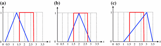

  

  Secondary MFs for Exercise 7.13

• 7.14

  • (a) (Mendel 2011) For each of the nine situations shown in Table 7.3, show that the join is given by the heavy red curve.

    Table 7.3 Join examples for Exercise 7.14 (Mendel 2011: ⓒ 2011 IEEE)

  • (b) Observe in Table 7.3 that each figure is labeled S1, or S2, … , or S5. What are five conclusions that can be drawn from the join results that are in this table?

• 7.15

  • (a) (Mendel 2011) For each of the nine situations shown in Table 7.4, show that the meet is given by the heavy red curve.

    Table 7.4 Meet examples for Exercise 7.15 (Mendel 2011: ⓒ 2011 IEEE)

  • (b) Observe in Table 7.4 that each figure is labeled S1, or S2, …, or S5. What are five conclusions that can be drawn from the meet results that are in this table?

• 7.16 This exercise examines the meet between a T1 FS, A, and a GT2 FS, $\tilde{B}$, under minimum and product t-norms. To do this, A is represented as a GT2 FS (see Sect. 6.8), as $(x \in X)$: $\tilde{A} = 1/A \to \mu_{{\tilde{A}}} = 1/\mu_{A}$, and $\tilde{B}$ is described by its MF $\mu_{{\tilde{B}}} (x,u)$, where

  $$ \mu_{{\tilde{B}}} (x,u) = \int\limits_{x \in X} {{{\mu_{{\tilde{B}(x)}} (u)} \mathord{\left/ {\vphantom {{\mu_{{\tilde{B}(x)}} (u)} {x = }}} \right. \kern-0pt} {x = }}} {{\int\limits_{x \in X} {\left[ {\int\limits_{u \in K \equiv [l,r] \subset [0,1]} {g_{x} (u)/u} } \right]} } \mathord{\left/ {\vphantom {{\int\limits_{x \in X} {\left[ {\int\limits_{u \in K \equiv [l,r] \subset [0,1]} {g_{x} (u)/u} } \right]} } x}} \right. \kern-0pt} x} $$

  • (a) For product t-norm, show that $\mu_{A} (x)\sqcap \mu_{{\tilde{B}(x)}} = \int\nolimits_{u \in K} {{{g_{x} (u)} \mathord{\left/ {\vphantom {{g_{x} (u)} {[\mu_{A} (x) \cdot u}}} \right. \kern-0pt} {[\mu_{A} (x) \cdot u}}} ]$

  • (b) For minimum t-norm, the evaluation of $\mu_{A} (x)\sqcap \mu_{{\tilde{B}(x)}}$ requires considering the three cases that are depicted in Fig. 7.19. For case 1, $\mu_{A} (x) < u\,{\text{when}}\,u \in K$; for case 2, $\mu_{A} (x) \in K\,{\text{when}}\,u \in K$; and for case 3, $\mu_{A} (x) > u\,{\text{when}}\,u \in K$. Show that:

    Fig. 7.19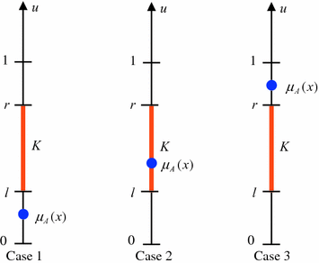

    

    Three cases for Exercise 7.16

    $$ \mu_{A} (x)\sqcap \mu_{{\tilde{B}(x)}} = \left\{ {\begin{array}{*{20}l} {1/\mu_{A} (x)} \hfill & {{\text{if}}\,\mu_{A} (x) < u} \hfill & {{\text{and}}\,u \in K} \hfill \\ {\int\limits_{d \in D} {{{g_{x} (d)} \mathord{\left/ {\vphantom {{g_{x} (d)} d}} \right. \kern-0pt} d}} } \hfill & {{\text{if}}\,\mu_{A} (x) \in K} \hfill & {{\text{and}}\,u \in K\,,\,{\text{and}}\,D \equiv [l,\mu_{A} (x)]} \hfill \\ {\mu_{{\tilde{B}(x)}} } \hfill & {{\text{if}}\,\mu_{A} (x) > u} \hfill & {{\text{and}}\,u \in K} \hfill \\ \end{array} } \right. $$

• 7.17 Figure 7.20 depicts a type-1 interval fuzzy number g(v) and a triangular type-1 set f(v). Note that L, R, A, T, and I stand for left, right, apex, triangle, and interval, respectively. Using (7.12) and (7.16) for the meet using the product t-norm, prove that $\mu_{F\sqcap G} (\theta )$ is given by the trapezoidal function that is depicted in Fig. 7.21.

  Fig. 7.20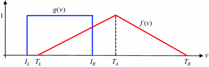

  

  Type-1 interval fuzzy number and triangular type-1 fuzzy set for Exercise 7.17

  Fig. 7.21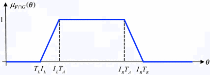

  

  Solution to Exercise 7.17

• 7.18 Apply (7.6) to the case when the secondary MFs are type-1 interval fuzzy numbers , and check the results obtained with those given in Theorem 7.11.

• 7.19 (a) Prove part (a) in the proof of Theorem 7.12. (b) Complete the proof of part (b) in the proof of Theorem 7.12.

• 7.20 Apply (7.10) to the case when the secondary MFs are type-1 interval fuzzy numbers , and check the results obtained with those given in Theorem 7.12.

• 7.21 Let $F_{1}$ and $F_{2}$ be two type-1 interval fuzzy numbers , having domains $[a,b]$ and $[c,d]$, respectively. Assume that $[a,b]$ and $[c,d]$ do not overlap, i.e., $d < a$ or $c > b$. Compute $F_{1} \sqcup F_{2}$ and $F_{1} \sqcap F_{2}$ for both situations using the minimum t-norm. Draw some conclusions about the join and meet of two type-1 interval fuzzy numbers , whose domains do not overlap. Note that there do not appear to be comparable results for product t-norm.

• 7.22 Given the three type-1 interval fuzzy numbers, $F_{1}$, $F_{2}$ and $F_{3}$ having the domains $[0.1,0.3]$, $[0.15,0.25]$ and $[0.2,0.4]$, respectively. Compute the following: (a) $F_{1} \sqcup F_{2} \sqcup F_{3}$ and (b) $F_{1} \sqcap F_{2} \sqcap F_{3}$. Do (b) for both minimum and product t-norms.

• 7.23 Formulas for the join and meet of IT2 FSs assumed in their derivations that supports of secondary MFs are connected (see Definitions 6.4 and 6.6). What happens in (7.161), for the join, when supports are disconnected? To answer this question assume that $\mu_{{\tilde{A}(x^{\prime})}}$ and $\mu_{{\tilde{B}(x^{\prime})}}$ have supports that are depicted in Fig. 7.22. Only consider the two cases when $f < a$ or $e > d$. Draw conclusions.

  Fig. 7.22

  

  Supports of secondary MFs for Exercise 7.23

• 7.24 Redo Examples 7.1, 7.7 and 7.12 using horizontal slices, as explained in Sects. 7.4.1, 7.4.2 and 7.4.3, respectively.

• 7.25 This exercise is a generalization of Exercise 2.33 to IT2 FSs whose lower and upper MFs are trapezoids that may or may not be normal (Lee and Chen 2008; Wei and Chen 2009). Its results are finding applications because of their closed-form nature. Let (see Fig. 7.23)

  Fig. 7.23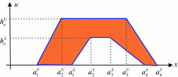

  

  Trapezoidal lower and upper MFs for Exercise 7.25

  $$ \begin{aligned} \tilde{A}_{1} & = (A_{1}^{U} ,A_{1}^{L} ) = ([a_{11}^{U} ,a_{12}^{U} ,a_{13}^{U} ,a_{14}^{U} ;h_{{a_{1} }}^{U} ],[a_{11}^{L} ,a_{12}^{L} ,a_{13}^{L} ,a_{14}^{L} ;h_{{a_{1} }}^{L} ]) \\ \tilde{A}_{2} & = (a_{2}^{U} ,a_{2}^{L} ) = ([a_{21}^{U} ,a_{22}^{U} ,a_{23}^{U} ,a_{24}^{U} ;h_{{a_{2} }}^{U} ],[a_{21}^{L} ,a_{22}^{L} ,a_{23}^{L} ,a_{24}^{L} ;h_{{a_{2} }}^{L} ]) \\ \end{aligned} $$

  Prove that (see the end of Exercise 2.33 for explanation of

  $$ \approx $$

  , which here applies to both the LMF and UMF):

  • (a)
    $$ \tilde{A}_{1} + \tilde{A}_{2} \approx ([a_{11}^{U} + a_{21}^{U} ,a_{12}^{U} + a_{22}^{U} ,a_{13}^{U} + a_{23}^{U} ,a_{14}^{U} + a_{24}^{U} ;\hbox{min} (h_{{a_{1} }}^{U} ,h_{{a_{2} }}^{U} )],[a_{11}^{L} + a_{21}^{L} ,a_{12}^{L} + a_{22}^{L} ,a_{13}^{L} + a_{23}^{L} ,a_{14}^{L} + a_{24}^{L} ;\hbox{min} (h_{{a_{1} }}^{L} ,h_{{a_{2} }}^{L} )] )$$
  • (b)
    $$ \tilde{A}_{1} - \tilde{A}_{2} \approx ([a_{11}^{U} - a_{24}^{U} ,a_{12}^{U} - a_{23}^{U} ,a_{13}^{U} - a_{22}^{U} ,a_{14}^{U} - a_{21}^{U} ;\hbox{min} (h_{{a_{1} }}^{U} ,h_{{a_{2} }}^{U} )],[a_{11}^{L} - a_{24}^{L} ,a_{12}^{L} - a_{23}^{L} ,a_{13}^{L} - a_{22}^{L} ,a_{14}^{L} - a_{21}^{L} ;\hbox{min} (h_{{a_{1} }}^{L} ,h_{{a_{2} }}^{L} )] )$$
  • (c)
    $$ \tilde{A}_{1} \cdot\tilde{A}_{2} \approx ( {\left[ {a_{11}^{U} a_{21}^{U}, a_{12}^{U} a_{22}^{U}, a_{13}^{U} a_{23}^{U}, a_{14}^{U} a_{24}^{U}; \text{min}(h_{a_{1}}^{U}, h_{a_{2}}^{U})],[a_{11}^{L} a_{21}^{L} ,a_{12}^{L} a_{22}^{L}, a_{13}^{L} a_{23}^{L}, a_{14}^{L} a_{24}^{L} }; \text{min} (h_{a_{1}}^{L}, h_{a_{2}}^{L}) \right]} ) $$
  • (d)
    $$ \tilde{A}_{1} ^{{ - 1}} \approx ( \left[ {1/a_{{14}}^{U} ,1/a_{{13}}^{U} ,1/a_{{12}}^{U} ,1/a_{{11}}^{U} ;h_{{a_{1} }}^{U} } \right],\left[ {1/a_{{14}}^{L} ,1/a_{{13}}^{L} ,1/a_{{12}}^{L} ,1/a_{{11}}^{L} ;h_{{a_{1} }}^{L} } \right] ) $$
  • (e)
    $$ \tilde{A}_{1} /\tilde{A}_{2} \approx ([a_{11}^{U} /a_{24}^{U} ,a_{12}^{U} /a_{23}^{U} ,a_{13}^{U} /a_{22}^{U} ,a_{14}^{U} /a_{21}^{U} ;\hbox{min} (h_{{a_{1} }}^{U} ,h_{{a_{2} }}^{U} )],[a_{11}^{L} /a_{24}^{L} ,a_{12}^{L} /a_{23}^{L} ,a_{13}^{L} /a_{22}^{L} ,a_{14}^{L} /a_{21}^{L} ;\hbox{min} (h_{{a_{1} }}^{L} ,h_{{a_{2} }}^{L} )] ) $$

  • (f) What do the formulas in (a)–(e) reduce to when $\tilde{A}_{1}$ and $\tilde{A}_{2}$ are perfectly normal interval type-2 fuzzy numbers?

• 7.26 Prove Theorem 7.15.

• 7.27 Prove Theorem 7.16.

• 7.28 Develop a procedure for computing $\neg \mu_{{\tilde{A}(x)}}$ using (7.70).

• 7.29 Complete the calculations to obtain the results in (7.85) and (7.86).

• 7.30 Explain how to carry out the computations in the extended sup-star composition (7.87) when U, W, and V are continuous universes of discourse.

• 7.31 Complete the calculations to obtain the results in (7.91).

• 7.32 Redo the calculations in Example 7.24 using product t-norm.

• 7.33 Carefully show how (7.92) follows from (7.87), when the first relation in the latter equation is just a GT2 FS.

• 7.34 Complete the calculations to obtain the results in (7.95).

• 7.35 Suppose $U = \{ 2,12\}$, $V = \{ 1,7,13\}$ and

  $$ \begin{aligned} & \mu_{{\tilde{R}}} (u) \equiv \begin{array}{*{20}c} {u_{1} } \\ {\left( {1/0.7 + 1/0.9} \right.} \\ \end{array} \begin{array}{*{20}c} {u_{2} } \\ {\left. {1/0.1 + 1/0.4} \right)} \\ \end{array} \\ & \mu_{{\tilde{S}}} (u,v) \equiv \begin{array}{*{20}c} {} \\ {\begin{array}{*{20}c} {u_{1} } \\ {u_{2} } \\ \end{array} } \\ \end{array} \begin{array}{*{20}c} {v_{1} } \\ {\left( {\begin{array}{*{20}c} {1/0.8 + 1/0.9 + 1/1} \\ {1/0.1 + 1/0.3} \\ \end{array} } \right.} \\ \end{array} \begin{array}{*{20}c} {v_{2} } \\ {\begin{array}{*{20}c} {1/0.3 + 1/0.4 + 1/0.5} \\ {1/0.2 + 1/0.5 + 1/0.8} \\ \end{array} } \\ \end{array} \begin{array}{*{20}c} {v_{2} } \\ {\left. {\begin{array}{*{20}c} {1/0 + 1/0.1} \\ {1/0.6 + 1/0.7 + 1/0.9} \\ \end{array} } \right)}. \\ \end{array} \\ \end{aligned} $$

  Compute $\mu_{{\tilde{R} \circ \tilde{S}}}$ by using (7.92) and the join and meet formulas in (7.3) and (7.7).

• 7.36 Perform the detailed calculations to obtain $\mu_{{(\tilde{F} \times \tilde{G})(x_{1} ,x_{2} )}}$ in (7.112).

• 7.37 Show that for GT2 FSs, whose secondary MFs are normal and convex, all the set-theoretic laws are satisfied under maximum t-conorm and minimum t-norm.

• 7.38 Explain why all of the “NO” elements in Table 7.1 are correct.

• 7.39 Show that for IT2 FSs the entries in the “Normal/Convex” column of Table 7.2 become the same as the entries in the “Product t-norm” column of Table 2-8.

• 7.40 Repeat Example 7.27 for the following normal and non-convex secondary MFs : $\mu_{{\tilde{A}(x)}} (u) = 0.5/0.1 + 0.2/0.3 + 1/0.7$, $\mu_{{\tilde{B}(x)}} (u) = 0.6/0.3 + 0.3/0.5 + 1/0.7$, $\mu_{{\tilde{C}(x)}} (u) = 0.4/0.2 + 0.2/0.6 + 1/0.8$.

• 7.41 Show that, under product t-norm and maximum t-conorm, $\mu_{{\tilde{A}(x)}} \sqcap \mu_{{\tilde{B}(x)}} = \mu_{{\tilde{B}(x)}} \sqcap \mu_{{\tilde{A}(x)}}$.

• 7.42 Show that, under product t-norm and maximum t-conorm, $\mu_{{\tilde{A}(x)}} \sqcup (\mu_{{\tilde{B}(x)}} \sqcup \mu_{{\tilde{C}(x)}} ) = (\mu_{{\tilde{A}(x)}} \sqcup \mu_{{\tilde{B}(x)}} ) \sqcup \mu_{{\tilde{C}(x)}}$.

• 7.43 Show that for GT2 FSs the involution law is satisfied under maximum t-conorm and product t-norm.

• 7.44 Complete all the details for Example 7.27.

• 7.45 This exercise is a generalization of the T1 FS cardinality Exercise 2.43 to IT2 FSs and GT2 FSs . It is based on results that are in Wu and Mendel (2007), Mendel (2009) and Zhai and Mendel (2011). The reader must read Exercise 2.43 before proceeding. Let $P_{{\tilde{A}}}$ denote the cardinality of IT2 FS $\tilde{A}$.

  • (a) Use the Wavy-Slice Representation Theorem 6.3 to prove that $P_{{\tilde{A}}} = [{\text{card}}({\underline{\mu }}_{{\tilde{A}}} (x)),{\text{card}}(\bar{\mu }_{{\tilde{A}}} (x))]$.

  • (b) Using the T1 FS cardinality $p(A)$ that is given in Exercise 2.43, write formulas for $P_{{\tilde{A}}}$ for continuous and discrete universes of discourse.

  • (c) Compute $P_{{\tilde{A}}}$ for the IT2 FS that is depicted in Fig. 7.24, when $N = 8$.

    Fig. 7.24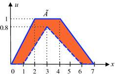

    

    IT2 FS for Exercise 7.45

  • (d) Associated with $P_{{\tilde{A}}}$ is the average cardinality of $\tilde{A}$, $AC(\tilde{A})$, which is a number, where $AC(\tilde{A}) = \tfrac{1}{2}[{\text{card}}({\underline{\mu}}_{{\tilde{A}}} (x)) + {\text{card}}(\bar{\mu }_{{\tilde{A}}} (x))]$. Compute $AC(\tilde{A})$ for $\tilde{A}$ in Fig. 7.24.

  • (e) Explain how the cardinality of a GT2 FS can be defined and computed. Would the result be a number, T1 FS, IT2 FS or a GT2 FS? If it is not a number, then propose a way to obtain $AC(\tilde{A})$ for a GT2 FS. (Hint: See Sect. 7.12.)

• 7.46 This exercise is a generalization of the T1 FS similarity Exercise 2.44 to IT2 FSs and GT2 FSs . It is based on results that are in Wu and Mendel (2009) and Mendel and Wu (2010, Chap. 4). The reader must read Exercise 2.44 before proceeding. Just as there are many definitions for the similarity of T1 FSs, there are many (although not nearly so many as for T1 FSs) definitions for the similarity of IT2 FSs [see the two just mentioned references for discussions about this, as well as Livi et al. (2014)]. One could use the Wavy-Slice Representation Theorem 6.3, as was done in Exercise 7.45, to obtain a formula for the similarity of an IT2 FS; however, doing this would lead to a type-1 interval fuzzy number for such a similarity. This exercise prefers to examine a crisp number for the similarity of IT2 FSs.²⁰

  Let $sm(\tilde{A},\tilde{B})$ denote the similarity between the two IT2 FSs $\tilde{A}$ and $\tilde{B}$. A crisp numerical Jaccard similarity measure between $\tilde{A}$ and $\tilde{B}$ is: $sm_{J} (\tilde{A},\tilde{B}) = {{AC(\tilde{A} \cap \tilde{B})} \mathord{\left/ {\vphantom {{AC(\tilde{A} \cap \tilde{B})} {AC(\tilde{A} \cup \tilde{B})}}} \right. \kern-0pt} {AC(\tilde{A} \cup \tilde{B})}}$, where AC is the average cardinality that is defined in Exercise 7.45.²¹

  • (a) Show that, for discrete universes of discourse:

    $$ sm_{J} (\tilde{A},\tilde{B}) = \frac{{\sum\nolimits_{i = 1}^{N} {\hbox{min} \left( {\bar{\mu }_{{\tilde{A}}} (x_{i} ),\bar{\mu }_{{\tilde{B}}} (x_{i} )} \right) + \sum\nolimits_{i = 1}^{N} {\hbox{min} \left( {\underline{\mu }_{{\tilde{A}}} (x_{i} ),\underline{\mu }_{{\tilde{B}}} (x_{i} )} \right)} } }}{{\sum\nolimits_{i = 1}^{N} {\hbox{max} \left( {\bar{\mu }_{{\tilde{A}}} (x_{i} ),\bar{\mu }_{{\tilde{B}}} (x_{i} )} \right) + \sum\nolimits_{i = 1}^{N} {\hbox{max} \left( {\underline{\mu }_{{\tilde{A}}} (x_{i} ),\underline{\mu }_{{\tilde{B}}} (x_{i} )} \right)} } }} $$

  • (b) What is the comparable formula for continuous universes of discourse?

  • (c) Compute $sm_{J} (\tilde{A},\tilde{B})$ for $\tilde{A}\,{\text{and}}\,\tilde{B}$ that are depicted in Fig. 7.25.

    Fig. 7.25

    

    Two FOUs for Exercises 7.46 and 7.47

  • (d) Explain how an analogous Jaccard similarity measure of a GT2 FS can be defined and computed. Will it be a single number or a type-1 fuzzy set? See Hao and Mendel (2014) for numerical examples and more discussions about this (Hint: See Sect. 7.12).

• 7.47 This exercise is a generalization of the T1 FS subsethood Exercise 2.45 to IT2 FSs and GT2 FSs. It is based on results that are in Mendel and Wu (2010, Chap. 4). The reader must read Exercise 2.45 before proceeding. Just as there are different definitions for the subsethood of T1 FSs, there are different (although not nearly so many as for T1 FSs) definitions for the subsethood of IT2 FSs (see Mendel and Wu (2010, Chap. 4) for discussions about this). One could use the Wavy-Slice Representation Theorem 6.3, as was done in Exercise 7.45, to obtain a formula for the subsethood of an IT2 FS; however, doing this would lead to a type-1 interval fuzzy number for such a subsethood. This exercise prefers to examine a crisp number for the subsethood of IT2 FSs.²²

  Let $sm(\tilde{A},\tilde{B})$ denote the subsethood between the two IT2 FSs $\tilde{A}$ and $\tilde{B}$. The Vlachos and Sergiadis subsethood measure between $\tilde{A}$ and $\tilde{B}$ is $ss_{VS} (\tilde{A},\tilde{B}) = {{AC(\tilde{A} \cap \tilde{B})} \mathord{\left/ {\vphantom {{AC(\tilde{A} \cap \tilde{B})} {AC(\tilde{A})}}} \right. \kern-0pt} {AC(\tilde{A})}}$, where AC is the average cardinality that is defined in Exercise 7.45.²³

  • (a) Show that, for discrete universes of discourse:

    $$ ss_{VS} (\tilde{A},\tilde{B}) = \frac{{\sum\nolimits_{i = 1}^{N} {\hbox{min} \left( {\underline{\mu }_{{\tilde{A}}} (x_{i} ),\underline{\mu }_{{\tilde{B}}} (x_{i} )} \right)} + \sum\nolimits_{i = 1}^{N} {\hbox{min} \left( {\bar{\mu }_{{\tilde{A}}} (x_{i} ),\bar{\mu }_{{\tilde{B}}} (x_{i} )} \right)} }}{{\sum\nolimits_{i = 1}^{N} {\underline{\mu }_{{\tilde{A}}} (x_{i} )} + \sum\nolimits_{i = 1}^{N} {\bar{\mu }_{{\tilde{A}}} (x_{i} )} }} $$

  • (b) What is the comparable formula for continuous universes of discourse?

  • (c) Compute $ss_{VS} (\tilde{A},\tilde{B})$ for $\tilde{A}$ and $\tilde{B}$ that are depicted in Fig. 7.25.

  • (d) Explain how an analogous Vlachos and Sergiadis subsethood measure of a GT2 FS can be defined and computed. Will it be a single number or a T1 FS? (Hint: see Sect. 7.12.)

References

Bilgin, A., H. Hagras, A. Malibari, M. Alhaddad, and D. Alghazzawi. 2012a. Towards a general type-2 fuzzy logic approach for computing with words using linear adjectives. In Proceedings of FUZZ-IEEE 2012, 1130–1137. Brisbane, AU.
Bilgin, A., J. Dooley, L. Whittington, H. Hagras, M. Henson, C. Wagner, A. Malibari, A. Al-Ghamdi, M. Alhaddad, and D. Alghazzawi. 2012b. Dynamic profile-selection for zslices based type-2 fuzzy agents controlling multi-user ambient intelligent environments. In Proceedings of FUZZ-IEEE 2012, 1392–1399. Brisbane, AU.
Bilgin, A., H. Hagras, A. Malibari, M. J. Alhaddad, and D. Alghazzawi. 2012c. A general type-2 fuzzy logic approach for adaptive modeling of perceptions for computing with words. In Proceedings of 2012 12th UK Workshop on Computational Intelligence (UKCI), 1–8.
Bilgin, A., H. Hagras, A. Malibari, M. J. Alhaddad, and D. Alghazzawi. 2013a. An experience based linear general type-2 fuzzy logic approach for computing with words. In Proceedings of IEEE Int’l. Conference on Fuzzy Systems, Paper #1139, Hyderabad, India.
Bilgin, A., H. Hagras, A. Malibari, M. J. Alhaddad, and D. Alghazzawi. 2013b. Towards a linear general type-2 fuzzy logic based approach for computing with words. Soft Computing.
Bustince, H., et al. 2016. A historical account of types of fuzzy sets and their relationships. IEEE Transactions on Fuzzy Systems 24: 179–194.
Chen, Q., and S. Kawase. 2000. On fuzzy-valued fuzzy reasoning. Fuzzy Sets and Systems 113: 237–251.
Cornelis, C., and E. Kerre. 2004. Inclusion measures in intuitionistic fuzzy set theory. Lecture Notes in Computer Science 2711: 345–356.
Coupland, S. and R. I. John. (2004) A new and efficient method for the type-2 meet operation. In Proceedings of IEEE FUZZ Conference, 959–964. Budapest, Hungary.
Coupland, S., and R. I. John. 2005. Towards more efficient type-2 fuzzy logic systems. In Proceedings of IEEE FUZZ Conference, 236–241. Reno, NV, May 2005.
Coupland, S., and R.I. John. 2007. Geometric type-1 and type-2 fuzzy logic systems. IEEE Transactions on Fuzzy Systems 15: 3–15.
Coupland, S., and R. I. John. 2013. Geometric type-2 fuzzy sets. In Advances in type-2 fuzzy sets and systems: Theory and applications, edited by A. Sadeghian, J. M. Mendel, and H. Tahayori. Springer, New York.
Dubois, D., and H. Prade. 1978. Operations on fuzzy numbers. International Journal of Systems Science 9: 613–626.
Dubois, D., and H. Prade. 1979. Operations in a fuzzy-valued logic. Information and Control 43: 224–240.
Dubois, D., and H. Prade. 1980. Fuzzy sets and systems: Theory and applications. NY: Academic Press.
Greenfield, S., and R. I. John. 2007. Optimized generalized type-2 join and meet operations. In Proceeding of FUZZ-IEEE 2007, 141–146. London, UK.
Hamrawi, H., S. Coupland, and R. John. 2010. A novel alpha-cut representation for type-2 fuzzy sets. In Proceeding of FUZZ-IEEE 2010, IEEE World Congress on Computational Intelligence, 351–358. Barcelona, Spain.
Hao, M., and J.M. Mendel. 2014. Similarity measures for general type-2 fuzzy sets based on the α-plane representation. Information Sciences 277: 197–215.
Harding, J., C. Walker, and E. Walker. 2010. The variety generated by the truth value algebra of type-2 fuzzy sets. Fuzzy Sets and Systems 161: 735–749.
John, R., J. Mendel, and J. Carter. 2006. The extended sup-star composition for type-2 fuzzy sets made simple. In Proceeding of 2006 IEEE International Conference on Fuzzy Systems, 1441–1445. Vancouver, BC, Canada.
Karnik, N. N., and J. M. Mendel. 1988a. Introduction to type-2 fuzzy logic systems. In Proceedings of 1998 IEEE FUZZ Conference, 915–920. Anchorage, AK.
Karnik, N. N., and J. M. Mendel. 1998b. Operations on Type-2 Fuzzy Sets. USC-SIPI Report # 319, University of Southern California, Los Angeles, CA. This can be accessed at: http://sipi.usc.edu/research; then choose “sipi technical reports/319.”.
Karnik, N. N., and J. M. Mendel. 1998c. An Introduction to Type-2 Fuzzy Logic Systems, USC-SIPI Report #418, University of Southern California, Los Angeles, CA. This can be accessed at: http://sipi.usc.edu/research; then choose “sipi technical reports/418.”.
Karnik, N.N., and J.M. Mendel. 2001. Operations on type-2 fuzzy sets. Fuzzy Sets and Systems 122: 327–348.
Klir, G.J., and T.A. Folger. 1988. Fuggy sets, uncertainity, and information. Englewood Cliffs, NJ: Prentice-Hall.
Klir, G.J., and B. Yuan. 1995. Fuzzy sets and fuzzy logic: Theory and applications. Upper Saddle River, NJ: Prentice Hall.
Kreinovich, V., and G. Xiang. 2008. Towards fast algorithms for processing type-2 fuzzy data: Extending Mendel’s algorithms from interval-valued to a more general case, In Proceeding of NAFIPS 2008, Paper #60106, New York City.
Lee, L.-W., and S.-M. Chen. 2008. A new method for fuzzy multiple attributes group decision-making based on the arithmetic of interval type-2 fuzzy sets. In Proceeding of the Seventh International Conference on Machine Learning and Cybernetics, 3084–3089. Kunming, China.
Lin, C.-T., and C.S.G. Lee. 1996. Neural fuzzy systems: A neuro-fuzzy synergism to intelligent systems. Upper Saddle River, NJ: Prentice-Hall PTR.
Livi, L., H. Tahayori, A. Sadeghian, and A. Rizzi. 2014. Distinguishability of interval type-2 fuzzy sets data by analyzing upper and lower membership functions. Applied Soft Computing 17: 79–89.
Mendel, J.M. 2001. Introduction to rule-based fuzzy logic systems. Upper Saddle River, NJ: Prentice-Hall.
Mendel, J.M. 2009. On answering the question ‘Where do I start in order to solve a new problem involving interval type-2 fuzzy sets?’. Information Sciences 179: 3418–3431.
Mendel, J. M. 2011. On the geometry of join and meet calculations for general type-2 fuzzy sets. In Proceedings of FUZZ-IEEE 2011, 2407–2413. Taipei, Taiwan.
Mendel, J.M., R.I. John, and F. Liu. 2006. Interval type-2 fuzzy logic systems made simple. IEEE Transactions on Fuzzy Systems 14: 808–821.
Mendel, J.M., F. Liu, and D. Zhai. 2009. Alpha-plane representation for type-2 fuzzy sets: Theory and applications. IEEE Transactions on Fuzzy Systems 17: 1189–1207.
Mendel, J.M., and D. Wu. 2010. Perceptual computing: Aiding people in making subjective judgments. Hoboken, NJ: Wiley and IEEE Press.
Miyakoshi, M., Y. Sato, and M. Kawaguchi. 1980. A fuzzy-fuzzy relation and its application to the clustering technique. Behaviormetrika 8: 15–22.
Mizumoto, M., and K. Tanaka. 1976. Some properties of fuzzy sets of type-2. Information and Control 31: 312–340.
Mizumoto, M., and K. Tanaka. 1981. Fuzzy sets of type-2 under algebraic product and algebraic sum. Fuzzy Sets and Systems 5: 277–290.
Nieminen, J. 1977. On the algebraic structure of fuzzy sets of type-2. Kybernetica, 13 (4): 261–273.
Nguyen, H. T., and V. Kreinovich. 2008.Computing degrees of subsethood and similarity for interval-valued fuzzy sets: Fast algorithms. In Proceedings of of 9th International Conference on Intelligent Technologies in Tech’08, 47–55. Samui, Thailand.
Rajati, M.R., and J.M. Mendel. 2013. Novel weighted averages versus normalized sums in Computing With Words. Information Sciences 235: 130–149.
Rickard, J. T., J. Aisbett, G. Gibbon, and D. Morgenthaler. 2008. Fuzzy subsethood for type-n fuzzy sets. In Proceeding of NAFIPS, New York.
Ruiz-Garcia, G., H. Hagras, H. Pomares, I. Rojas, and H. Bustince. 2016. Join and meet operations for type-2 fuzzy sets with non-convex secondary memberships. IEEE Transactions on Fuzzy Systems.
Tahayori, H., A. G. B. Tettamanzi, and G. D. Antoni. 2006. Approximated type-2 fuzzy set operations. In Proceedings of FUZZ-IEEE 2006, 9042–9049. Vancouver, B.C. Canada.
Wagner, C., and H. Hagras. 2008. z Slices—towards bridging the gap between interval and general type-2 fuzzy logic. In Proceeding of IEEE FUZZ Conference, Paper # FS0126, Hong Kong, China.
Wagner, C., and H. Hagras. 2010. Towards general type-2 fuzzy logic systems based on zSlices. IEEE Transactions on Fuzzy Systems 18: 637–660.
Wagner, C., and H. Hagras. 2013. zSlices based general type-2 fuzzy sets and systems. In Advances in Type-2 Fuzzy Sets and Systems: Theory and Applications, edited by A. Sadeghian, J. M. Mendel and H. Tahayori. Springer, New York.
Walker, C.L., and E. Walker. 2005. The algebra of fuzzy truth values. Fuzzy Sets Systems 149: 309–347.
Walker, C. L., and E. Walker. 2006. Automorphisms of the algebra of fuzzy truth values. International Journal of Uncertainty, Fuzziness and Knowledge-Based Systems, 14: 711–732.
Walker, C.L., and E.A. Walker. 2009. Sets with type-2 operations. International Journal of Approximate Reasoning 50: 63–71.
Walker, C.L., and E.A. Walker. 2014. Type-2 operations on finite chains. Fuzzy Sets and Systems 236: 33–49.
Wei, S.-H., and S.-M. Chen. 2009. Fuzzy risk analysis based on interval-valued fuzzy numbers. Expert Systems with Applications 36: 2285–2299.
Wu, D., and J.M. Mendel. 2007. Uncertainty measures for interval type-2 fuzzy sets. Information Sciences 177: 5378–5393.
Wu, D., and J.M. Mendel. 2009. A comparative study of ranking methods, similarity measures and uncertainty measures for interval type-2 fuzzy sets. Information Sciences 179: 1169–1192.
Zadeh, L.A. 1975. The concept of a linguistic variable and its application to approximate reasoning–1. Information Sciences 8: 199–249.
Zeng, W. Y. Zhou, and H. Li. 2007. Extension principle of interval-valued fuzzy set. In Fuzzy Information and Engineering: Proceedings of the Second International Conference on Fuzzy Information and Engineering (ICFIE), 125–137. Springer.
Zhai, D., and J.M. Mendel. 2011. Uncertainty measures for general type-2 fuzzy sets. Information Sciences 181: 503–518.
Author information
Authors and Affiliations
Corresponding author