Type-1 Fuzzy Sets and Fuzzy Logic

Abstract

This chapter formally introduces type-1 fuzzy sets and fuzzy logic . It is the backbone for Chap. 3 and provides the foundation upon which type-2 fuzzy sets and systems are built in later chapters. Its coverage includes: crisp sets , type-1 fuzzy sets and associated concepts [including a short biography of Prof. Zadeh (the father of fuzzy sets and fuzzy logic)], type-1 fuzzy set defined, linguistic variables , returning to linguistic variables from a numerical value of a membership function , set theoretic operations for crisp and type-1 fuzzy sets, crisp and fuzzy relations and compositions on the same or different product spaces , compositions of a type-1 fuzzy set with a type-1 fuzzy relation , hedges, the Extension Principle (which is about functions of fuzzy sets), α-cuts (which are a powerful way to represent a type-1 fuzzy set in terms of intervals), functions of type-1 fuzzy sets computed by using α-cuts , multivariable membership functions and Cartesian products , crisp logic , going from crisp logic to fuzzy logic, Mamdani (engineering) implications , some final remarks, and an appendix about properties/laws of type-1 fuzzy sets . 35 examples are used to illustrate this chapter’s important concepts.

Appendices

Appendix 1: Properties of Type-1 Fuzzy Sets

This appendix presents details about properties/laws of type-1 fuzzy sets and examines the following frequently used laws to see if they remain satisfied under maximum t-conorm and either minimum or product t-norms:

Reflexive, anti-symmetric, transitive, idempotent, commutative, associative, absorption, distributive, involution, De Morgan’s, and identity

Our reason for doing this is that rules in a rule-based system may make use of the words “and”, “or”, “unless”, “not”, etc., but all of the mathematics for such a system is worked out in this book only for canonical rules that use the words “and” and “or”. Section 3.2 shows how the former rules can be transformed into the canonical rules by using some of the above laws. So, it is important to know when or if the use of these laws is correct.

The exact nature of all the preceding laws is given in the second column of Table 2.8. These laws are all satisfied for crisp sets (for the minimum and product t-norms), due to the facts that: $\hbox{min} (0,0) = 0{\text{ and }}0 \times 0 = 0$, $\hbox{min} (1,0) = 0{\text{ and }}1 \times 0 = 0$, $\hbox{min} (0,1) = 0{\text{ and }}0 \times 1 = 0$, and, $\hbox{min} (1,1) = 1$ and $1 \times 1 = 1$. That they are all satisfied for maximum t-conorm and minimum t-norm (a so-called “dual t-conorm and t-norm pair”) is well known (e.g. Klir and Yuan 1995) and proofs for this situation are left to the reader (Exercise 2.41).

Table 2.8 Summary of set-theoretic laws and whether or not they are satisfied for type-1 fuzzy sets under maximum t-conorm and either minimum or product t-norms^a

The rest of this appendix focuses on the maximum t-norm and product t-norm pairing. Reflexive, anti-symmetric, and transitive laws do not make use of any t-norm; hence, they are automatically satisfied for maximum t-conorm and product t-norm. Commutative and associative laws are also satisfied, because both maximum and product operations are commutative and associative; i.e., for $x \in X$ ($\vee \equiv {\text{ maximum}}$):

$$ \mu_{A} (x) \vee \mu_{B} (x) = \mu_{B} (x) \vee \mu_{A} (x) $$

$$ \mu_{A} (x) \times \mu_{B} (x) = \mu_{B} (x) \times \mu_{A} (x) $$

$$ (\mu_{A} (x) \vee \mu_{B} (x)) \vee \mu_{C} (x) = \mu_{A} (x) \vee (\mu_{B} (x) \vee \mu_{C} (x)) $$

$$ (\mu_{A} (x) \times \mu_{B} (x)) \times \mu_{C} (x) = \mu_{A} (x) \times (\mu_{B} (x) \times \mu_{C} (x)) $$

Under product t-norm, the second part of the absorption laws is satisfied, because $\mu_{A} (x) \times \mu_{B} (x) \le \mu_{A} (x)$, so that $\mu_{A} (x) \vee (\mu_{A} (x) \times \mu_{B} (x)) = \mu_{A} (x)$. The first part of the distributive laws is satisfied; i.e., product is distributive over maximum. The first part of the idempotent laws is also satisfied; i.e., $\mu_{A} (x) \vee \mu_{A} (x)$ $= \mu_{A} (x)$. The involution law is satisfied, since complement is defined as $\mu_{{\bar{A}}} (x) = 1 - \mu_{A} (x)$. And, all the identity laws are satisfied (i.e., $\mu_{A} (x) \vee 0$ $= \mu_{A} (x)$, $\mu_{A} (x) \times 1 = \mu_{A} (x)$, $\mu_{A} (x) \vee 1 = 1$, and $\mu_{A} (x) \times 0 = 0$).

None of the other laws are satisfied under product t-norm, because:

• Idempotent laws—second part

  $$ \mu_{A} (x) \times \mu_{A} (x) \ne \mu_{A} (x) $$

  (2.150)

• Absorption laws—first part: assume, e.g. that $\mu_{A} (x) > \mu_{B} (x)$; then,

  $$ \mu_{A} (x) \times (\mu_{A} (x) \vee \mu_{B} (x)) = \mu_{A} (x) \times \mu_{A} (x) = \mu_{A}^{2} (x) \ne \mu_{A} (x) $$

  (2.151)

• Distributive laws–second part: assume, e.g. that $\mu_{A} (x) > \mu_{B} (x)$ and $\mu_{A} (x) > \mu_{C} (x)$; then,

  $$ \begin{aligned} \mu_{A} (x) \vee (\mu_{B} (x) \times \mu_{C} (x)) & = \mu_{A} (x) \\ & \ne (\mu_{A} (x) \vee \mu_{B} (x)) \times (\mu_{A} (x) \vee \mu_{C} (x)) = \mu_{A}^{2} (x) \\ \end{aligned} $$

  (2.152)

• De Morgan’s laws:

  $$ \begin{aligned} \overline{{\mu_{A} (x) \vee \mu_{B} (x)}} & = 1 - (\mu_{A} (x) \vee \mu_{B} (x)) \\ & \ne \mu_{{\bar{A}}} (x) \times \mu_{{\bar{B}}} (x) = (1 - \mu_{A} (x)) \times (1 - \mu_{B} (x)) \\ \end{aligned} $$

  (2.153)
  $$ \begin{aligned} \overline{{\mu_{A} (x) \times \mu_{B} (x)}} & = 1 - \mu_{A} (x) \times \mu_{B} (x) \\ & \ne \mu_{{\bar{A}}} (x) \vee \mu_{{\bar{B}}} (x) = \hbox{max} \{ (1 - \mu_{A} (x)),(1 - \mu_{B} (x))\} \\ \end{aligned} $$

  (2.154)

Exercises

• 2.1 Fuzziness as a concept that lets an object reside in more than one set but to different degrees may be traced back to antiquity. Go on the Internet and find a picture of the statue called the Guardian Sphinx (530 BC.).

  • (a) What are the three sets for this statue?

  • (b) What membership grade would you assign to each of the three sets?

• 2.2 Fuzziness as a concept that lets an object reside in more than one set but to different degrees has occurred in art, even before Zadeh formalized it. For example, it occurs in the works of the Belgian painter Renè Magritte. Go on the Internet and find the following paintings by him and answer the related question:

  • (a) The Explanation (1952): What is the degree of similarity between the carrot and the wine bottle?

  • (b) Homage to Alphonse Allais (1964): What is the degree of similarity between the cigar and the fish?

• 2.3 Suppose that a car is described by its color. What scale could be used for color? Create five terms for color and sketch MFs for each term.

• 2.4 Establish MFs for:

  • (a) real numbers close to 10

  • (b) real numbers approximately equal to 6

  • (c) integers very far from 10

  • (d) complex numbers near the origin

  • (e) light (weight)

  • (f) heavy (weight).

• 2.5 List six linguistic variables from the field of acoustics (or any field that is of interest to you).

• 2.6 Using the rules in Example 2.5 as illustrations, list four more rules and their associated MFs.

• 2.7 Let X be the set of all men and Y be the set of all women. Consider the linguistic variable “weight,” and the set of terms {very skinny, skinny, just right, heavy, very heavy}. Create MFs for these terms for both men and women.

• 2.8 Consider the judgments listed here, and assume that they can be mapped onto an interval scale ranging from 0 to 10. Define five fuzzy sets for each of them and sketch what you feel are appropriate MFs for them.

  • (a) touching

  • (b) eye contact

  • (c) smiling

  • (d) acting witty

  • (e) flirtation.

• 2.9 Western logic and thinking has been dominated for the most part by the Aristotelian laws of contradiction and the excluded middle . Eastern thinking has not. Eastern religions and concepts such as the Yin and the Yang (female and male/opposite forces) have caused some to speculate that this is why China and Japan were more receptive to fuzzy logic than were people in the West. For example, it’s possible for each of you to reside in Yin and Yang simultaneously, but to different degrees. Explain this in terms of fuzzy sets.

• 2.10 Prove that, for crisp sets A and B, $\hbox{min} [\mu_{A} (x),\mu_{B} (x)]$ provides the correct MF for intersection , given in (2.12).

• 2.11 For crisp sets A and B, prove the:

  • (a) commutative law

  • (b) associative laws

  • (c) distributive laws

  • (d) De Morgan’s laws.

• 2.12 Consider three fuzzy sets, A, B, and C, whose MFs are (unnormalized) Gaussians, i.e., $\mu_{A} (x) = \exp \left[ { - \tfrac{1}{2}(x - 3)^{2} } \right]$, $\mu_{B} (x) = \exp \left[ { - \tfrac{1}{2}(x - 4)^{2} } \right]$ and $\mu_{C} (x) = \exp \left[ { - \tfrac{1}{2}(x - 6)^{2} } \right]$. Sketch each of the following:

  • (a)
    $$ \mu_{A \cap B \cap C} (x) $$
  • (b)
    $$ \mu_{A \cup B \cup C} (x) $$
  • (c)
    $$ \mu_{(A \cup B) \cap C} (x){\text{ and }}\mu_{A \cup (B \cap C)} (x) $$
  • (d)
    $$ \mu_{(A \cap B) \cup C} (x){\text{ and }}\mu_{A \cap (B \cup C)} (x) $$
  • (e)
    $$ \mu_{{\overline{A \cup B \cup C} }} (x). $$

• 2.13 Consider the fuzzy sets A and B, where $\mu_{A} (x) = \exp \left[ { - \tfrac{1}{2}(x - 3)^{2} } \right]$ and $\mu_{B} (x) = \exp \left[ { - \tfrac{1}{2}(x - 4)^{2} } \right]$.

  • (a) Sketch $\mu_{A \cup B} (x)$ for the following t-conorms: maximum, algebraic sum, bounded sum and drastic sum. Which t-conorm gives the largest and smallest values for $\mu_{A \cup B} (x)$ ?

  • (b) Sketch $\mu_{A \cap B} (x)$ for the following t-norms: minimum, algebraic product, bounded product and drastic product. Which t-norm gives the largest and smallest values for $\mu_{A \cap B} (x)$?

• 2.14 Using (2.34) and (2.35), show that $\mu_{c \cup s} (u,v)$ and $\mu_{c \cap s} (u,v)$ are given by (2.38) and (2.39), respectively.

• 2.15 Verify the max-min and max-product composition of the crisp relations for the (3, 3) element of $R_{3} (U,W)$ in (2.43).

• 2.16 Consider the fuzzy relations “u is lighter than v” or “u is about the same weight as v.” Assume that $u \in U$ and $v \in V$ where U and V are discrete universes of discourse, and U has four elements whereas V has six elements.

  • (a) Pick U and V to use in the rest of this exercise.

  • (b) Establish MFs for lighter and about the same, i.e., $\mu_{l} (u,v)$ and $\mu_{ats} (u,v)$, where the numbers in $\mu_{l} (u,v)$ and $\mu_{ats} (u,v)$ agree with a comparison of the numbers in U and V.

  • (c) Compute $\mu_{l \cup ats} (u,v)$.

• 2.17 Perform all of the calculations needed to obtain $\mu_{c \circ mb} (u,w)$ given in (2.54).

• 2.18 Repeat Example 2.15 using the product t-norm. Compare these results with the ones given in (2.54) which were obtained using the minimum t-norm. Are they significantly different?

• 2.19 Consider the fuzzy relation “u is lighter than v” on $U \times V$, and the fuzzy relation “v is heavier than w” on $V \times W$. Assume that U, V, and W are discrete universes of discourse, and U has four elements, V has six elements, and W has three elements.

  • (a) Pick U, V, and W to use in the rest of this exercise.

  • (b) Establish MFs for lighter and heavier, i.e., $\mu_{l} (u,v)$ and $\mu_{h} (v,w)$, where the numbers in $\mu_{l} (u,v)$ and $\mu_{h} (v,w)$ agree with a comparison of the numbers in U, V, and W.

  • (c) Compute $\mu_{l \circ h} (u,w)$ using minimum t-norm.

  • (d) Compute $\mu_{l \circ h} (u,w)$ using product t-norm.

  • (e) Compare the results from (c) and (d).

• 2.20 Consider the fuzzy relation “u is lighter than v” on $U \times V$. Assume that U and V are discrete universes of discourse, and U has four elements and V has six elements.

  • (a) Pick U and V to use in the rest of this exercise.

  • (b) Establish a MF for lighter, i.e., $\mu_{l} (u,v)$, where the numbers in $\mu_{l} (u,v)$ agree with a comparison of the numbers in U and V.

  • (c) Construct a MF for the fuzzy set skinny, $\mu_{skinny} (u)$, on U.

  • (d) Compute the composition of “u is skinny” and “u is lighter than v”, $\mu_{skinny \circ l} (v)$.

• 2.21 Using the same universe of discourse as in Example 2.17, develop MFs for:

  • (a) very likely

  • (b) not-too-likely.

• 2.22 Suppose that $U = \{ - 5, - 4, - 3, - 2, - 1,0,1,2,3,4,5\}$ and fuzzy set A is characterized by the MF

  $$ \mu_{A} (x) = 0.2/ - 5 + 0.4/ - 4 + 0.4/ - 3 + 0.5/ - 2 + 0.5/ - 1 + 0.6/0 + 0.9/1 + 1/2 + 0.8/3 + 0.5/4 + 0.1/5 $$

  • (a) Determine the MF for the fuzzy set B that is associated with $\mu_{f(A)} (y)$ when $y = f(x) = x^{3} + 2x^{2}$.

  • (b) Determine the MF for the fuzzy set B that is associated with $\mu_{f(A)} (y)$ when $y = |x|$.

• 2.23 Suppose that $X_{1} = \{ 1,2,3,4\}$ and $X_{2} = \{ - 1, - 2, - 3, - 4\}$, and fuzzy sets $A_{1}$ and $A_{2}$ are characterized by the following MFs:

  $$ \mu_{{A_{1} }}(x_{1} ) = 0.5/1 + 0.5/2 + 0/3 + 1/4{\text{ and }} \mu_{{A_{2} }}(x_{2} ) = 1/ - 1 + 0/ - 2 + 0.25/ - 3 + 0.5/ - 4 $$

  Determine the MF for the fuzzy set B that is associated with $\mu_{{f(A_{1} A_{2} )}} (y)$, when $y = f(x_{1} ,x_{2} ) = x_{1}^{2} - 2x_{2}^{2}$.

• 2.24 Given the type-1 Gaussian fuzzy set $F_{i}$, with mean $m_{i}$ and standard deviation $\sigma_{i}$, prove that $a_{i} F_{i} + b$ is a Gaussian fuzzy set with mean $a_{i} m_{i} + b$ and standard deviation $\left| {a_{i} \sigma_{i} } \right|$. Note that this result does not depend on the kind of t-norm used, since $a_{i}$ and $b$ are crisp numbers.

• 2.25 Given n type-1 Gaussian fuzzy sets $F_{1} , \ldots ,F_{n}$, with means $m_{1} ,\ldots,m_{n}$ and standard deviations $\sigma_{1} , \ldots \sigma_{n}$, as in (2.77), prove that $\sum\nolimits_{i = 1}^{n} {F_{i} }$ is a Gaussian fuzzy set with mean $\sum\nolimits_{i = 1}^{n} {m_{i} }$ and standard deviation $\Sigma^{\prime \prime}$, where

  $$ \Sigma^{\prime \prime } = \left\{ {\begin{array}{*{20}l} {\sqrt {\sum\nolimits_{i = 1}^{n} {\sigma_{i}^{2} } } } & {{\text{if product t}} {\text{-}} {\text{norm is used}}} \\ {\sum\nolimits_{{i{ = }1}}^{n} {\sigma_{i} } } & {{\text{if minimum t}} {\text{-}} {\text{norm is used}}} \\ \end{array} } \right. $$

  [Hints: (1) First prove the results for two sets and then for three sets; (2) show that the supremum of the minimum of two Gaussians is reached at their point of intersection lying between their means.]

• 2.26 Complete part (b) in the proof of Example 2.21.

• 2.27 In Example 2.22, obtain the comparable results when $a_{i}$ are positive or negative real numbers.

• 2.28 Prove (2.81).

• 2.29 Repeat Example 2.28 but now for $\mu_{A \cap B} (x)$.

• 2.30 Let³⁵ $X_{i} (i = 1, \ldots ,n)$ be fuzzy sets with Gaussian MFs, $\mu_{{X_{i} }} (x_{i} ) = \exp \left( { - {{[(x_{i} - c_{i} )/\sigma_{i} ]^{2} } \mathord{\left/ {\vphantom {{[(x_{i} - c_{i} )/\sigma_{i} ]^{2} } 2}} \right. \kern-0pt} 2}} \right)$, and $w_{i} \ge 0$ be constant weights with $\sum\nolimits_{i = 1}^{n} {w_{i} } = 1$. Using the Extension Principle with the minimum t-norm, prove that $Y_{n} = \sum\nolimits_{i = 1}^{n} {w_{i} X_{i} }$ is a fuzzy set with MF $\mu_{{Y_{n} }} (y_{n} ) = \exp \left( { - {{\left[ {y_{n} - \sum\nolimits_{i = 1}^{n} {w_{i} c_{i} } } \right]^{2} } \mathord{\left/ {\vphantom {{\left[ {y_{n} - \sum\nolimits_{i = 1}^{n} {w_{i} c_{i} } } \right]^{2} } {\left[ {\sum\nolimits_{i = 1}^{n} {w_{i} \sigma_{i} } } \right]^{2} }}} \right. \kern-0pt} {\left[ {\sum\nolimits_{i = 1}^{n} {w_{i} \sigma_{i} } } \right]^{2} }}} \right)$. [Hint: Prove this by using mathematical induction.]

• 2.31 Let³⁶ $A = [a,b,c]$ and $B = [p,q,r]$ be two triangle type-1 fuzzy numbers with MF given in (2.103) and (2.104), respectively. Compute the MF of:

  • (a)
    $$ A - B $$
  • (b)
    $$ \exp (A) $$
  • (c)
    $$ \ln (A) $$
  • (d)
    $$ \sqrt A $$
  • (e)
    $$ (A)^{1/n}. $$

• 2.32 Let³⁷ $A = [a,b,c]$ and $B = [p,q,r]$ be two positive triangle type-1 fuzzy numbers with MF given in (2.103) and (2.104), respectively. Compute the MF of:

  • (a)
    $$ A \cdot B $$
  • (b)
    $$ A \div B $$
  • (c)
    $$ (A)^{ - 1}. $$

• 2.33 For the non-normal type-1 trapezoidal fuzzy number , $A_{i} = (a_{i} ,b_{i} ,c_{i} ,d_{i} ;w_{i} )$, whose MF is depicted in Fig. 2.21, prove that (Wei and Chen 2009):

  Fig. 2.21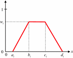

  

  Type-1 trapezoidal fuzzy number for Exercise 2.33

  • (a) $A_{1} + A_{2} = (a_{1} + a_{2} ,b_{1} + b_{2} ,c_{1} + c_{2} ,d_{1} + d_{2} ;\hbox{min} (w_{1} ,w_{2} )),$ where $a_{i}$, $b_{i}$, $c_{i}$ and $d_{i}$ are real numbers.

  • (b) $A_{1} - A_{2} = (a_{1} - d_{2} ,b_{1} - c_{2} ,c_{1} - b_{2} ,d_{1} - a_{2} ;\hbox{min} (w_{1} ,w_{2} ))$, where $a_{i}$, $b_{i}$, $c_{i}$ and $d_{i}$ are real numbers.

  • (c) $A_{1} \cdot A_{2} \approx (a_{1} \times a_{2} ,b_{1} \times b_{2} ,c_{1} \times c_{2} ,d_{1} \times d_{2} ;\hbox{min} (w_{1} ,w_{2} ))$, where $a_{i}$, $b_{i}$, $c_{i}$ and $d_{i}$ are positive real numbers.

  • (d) $A_{1} /A_{2} \approx (a_{1} /d_{2} ,b_{1} /c_{2} ,c_{1} /b_{2} ,d_{1} /a_{2} ;\hbox{min} (w_{1} ,w_{2} ))$, where $a_{i}$, $b_{i}$, $c_{i}$ and $d_{i}$ are non-zero positive real numbers.

  In (c) and (d), ≈ means that the result is a convex type-1 fuzzy set, as in (2.7), in which g(x) and h(x) are not straight lines.

• 2.34 Using truth tables show that the following are tautologies [3]:

  • (a)
    $$ p \wedge (q \vee r) \leftrightarrow (p \wedge q) \vee (p \wedge r) $$
  • (b)
    $$ p \vee (q \wedge r) \leftrightarrow (p \vee q) \wedge (p \vee r) $$
  • (c)
    $$ p \wedge (q \wedge r) \leftrightarrow (p \wedge q) \wedge r $$
  • (d)
    $$ p \vee (q \vee r) \leftrightarrow (p \vee q) \vee r $$

• 2.35 Use truth tables to determine whether or not the following propositions are tautologies:

  • (a)
    $$ (p \wedge q) \to (p \vee q) $$
  • (b)
    $$ \left[ {(p \to q) \wedge (r \to s) \wedge (p \vee r)} \right] \to (q \vee s) $$
  • (c)
    $$ \left( {(p \wedge q) \to r} \right) \leftrightarrow (p \to r) \vee (q \to r) $$

• 2.36 Prove that $[(A \wedge C) \to D] \wedge [(B \wedge C) \to D] \leftrightarrow [(A \vee B) \wedge C \to D]$[Hint: $(p \to q) \leftrightarrow ( \sim p) \vee q$].

• 2.37 Validate the truth of the crisp implication MFs given in (2.122) and (2.123).

• 2.38 Repeat Example 2.32 for the following implication MFs, and indicate which of these has a bias in its output:

  • (a) Kleene-Dienes in (2.121)

  • (b) Reichenbach in (2.122)

  • (c)
    $$ {{\rm G\ddot{o}del}}: \mu_{A \to B}^{G} (x^{\prime } ,y) = \left\{ {\begin{array}{*{20}l} 1 \hfill & {\mu_{\text{A}} (x^{\prime } ) \le \mu_{B} (y)} \hfill \\ {\mu_{\text{B}} (y)} \hfill & {\mu_{A} (x^{\prime } ) > \mu_{B} (y)} \hfill \\ \end{array} } \right. $$
  • (d)
    $$ {\text{Gaines Resher: }}\mu_{A \to B}^{GR} (x^{\prime},y) = \left\{ {\begin{array}{*{20}c} 1 & {\mu_{A} (x^{\prime}) \le \mu_{B} (y)} \\ 0 & {\mu_{A} (x^{\prime}) > \mu_{B} (y)} \\ \end{array} } \right. $$
• 2.39

  • (a) For the upward sloping lines in Fig. 2.22a, show that the sup-min composition between the lines and the triangle always occurs at the intersection of the line and the right-hand leg of the triangle.

    Fig. 2.22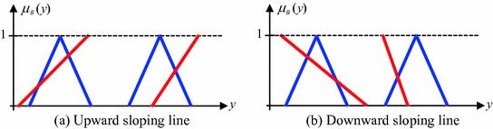

    

    Type-1 fuzzy sets for Exercise 2.39

  • (b) For the downward sloping lines in Fig. 2.22b, show that the sup-min composition between the lines and the triangle always occurs at the intersection of the line and the left-hand leg of the triangle.

• 2.40 Everything is the same as in Example 2.34, except that in this exercise minimum implication and minimum t-norm are used.

  • (a) Show that, in this case, the sup-star composition in (2.127) can be expressed as

    $$ \mu_{{B^{ * } }} (y) = \hbox{min} \left[ {\sup_{x \in X} [\hbox{min} [\mu_{{A^{ * } }} (x),\mu_{A} (x)]],\mu_{B} (y)} \right] $$

  • (b) Show that $\sup_{x \in X} [\hbox{min} [\mu_{{A^{ * } }} (x),\mu_{A} (x)]]$ occurs at the intersection point of the two Gaussian MFs, namely at

    $$ x = x_{\hbox{max} } = {{(\sigma_{{A^{ * } }}^{{}} m_{A} + \sigma_{A}^{{}} x^{\prime } )} \mathord{\left/ {\vphantom {{(\sigma_{{A^{ * } }}^{{}} m_{A} + \sigma_{A}^{{}} x^{\prime } )} {(\sigma_{{A^{ * } }}^{{}} + \sigma_{A}^{{}} )}}} \right. \kern-0pt} {(\sigma_{{A^{ * } }}^{{}} + \sigma_{A}^{{}} )}} . $$

  • (c) If possible, obtain a formula for $\sup_{x \in X} [\hbox{min} [\mu_{{A^{ * } }} (x),\mu_{A} (x)]]$.

  • (d) Assume a Gaussian consequent MF $\mu_{B} (y)$. Sketch the fired-rule MF $\mu_{{B^{ * } }} (y)$. How is this obtained directly from sketches of $\mu_{{A^{ * } }} (x)$, $\mu_{A} (x)$ and $\mu_{B} (y)$?

  • (e) Repeat part (d) for a triangular consequent MF.

  • (f) Compare the result in part (e) with the result in Fig. 2.19.

• 2.41 Show that for type-1 fuzzy sets all the set-theoretic laws that are in Table 2.8 are satisfied under maximum t-conorm and minimum t-norm.

• 2.42 Verify (2.153) and (2.154) numerically.

• 2.43 As one knows, crisp set A can be defined by using its MF in (2.1). The number of elements that are in A is called its cardinality. So, for a crisp set its cardinality can be obtained by summing all of its MF values. Using this idea³⁸, one can also define the cardinality of a type-1 fuzzy se t A, $|A|$, analogously (De Luca and Termini 1972), i.e. for a discrete universe, $|A| = \sum\nolimits_{i = 1}^{N} {\mu_{A} (x_{i} )}$, and for a continuous universe, $|A| = \int_{X} {\mu_{A} (x)dx}$. Observe that $|A|$ increases as N increases, and $\lim_{N \to \infty } \sum\nolimits_{i = 1}^{N} {\mu_{A} (x_{i} )}$ does not exist. Wu and Mendel (2007) handle this by defining a normalized cardinality , $p(A)$, for a type-1 fuzzy set in which DeLuca and Termini’s cardinality definition for continuous universes $|A| = \int_{X} {\mu_{A} (x)dx}$, is discretized, i.e.: $p(A) \equiv \frac{|X|}{N}\sum\nolimits_{i = 1}^{N} {\mu_{A} (x_{i} )}$, where $|X| = x_{N} - x_{1}$ is the length of the universe of discourse used in the computation. X can be part of the complete universe of discourse because for some MFs (e.g., Gaussian, Bell) the complete universes of discourse are infinite. Usually $x_{i}$ $(i = 1,\ldots,N)$ are chosen equally spaced in the domain of $x_{i}$; in this case, $p(A)$ converges to its continuous version, $\int_{X} {\mu_{A} (x)dx}$ as N increases.

  • (a) Compute $|A|$ for the triangle and trapezoidal type-1 fuzzy sets that are in Table 2.3.

  • (b) Compute $p(A)$ for the same MFs used in (a) for $N = 10, 50, 100$, and compare these results with $|A|$.

• 2.44 Similarity is sometimes used in a rule-based fuzzy system, so this exercise explores similarity for type-1 fuzzy sets. Similarity is about set equality. Two crisp sets A and B are equal if they contain exactly the same elements. In crisp set theory either two sets are equal or they are different. For fuzzy sets one knows that everything is a matter of degree; thus for two type-1 fuzzy sets A and B, it is reasonable to define a degree of similarity. As usual (in this book), crisp sets are our starting point.

As is stated in Nguyen and Kreinovich (2008): It is known that for two crisp sets A and B: (1) $A \cap B \subseteq A \cup B$ (create a Venn diagram to convince yourself of the truth of this), and (2) $A = B$ iff $A \cap B = A \cup B$. So, for crisp sets, to check whether $A = B$ consider the ratio $|A \cap B|/|A \cup B|$ where $| \centerdot |$ denotes the cardinality of $\centerdot$ (see Exercise 2.43 about cardinality). In general this ratio is between 0 and 1; the smaller the ratio, the more there are elements from $A \cup B$ which are not part of $A \cap B$, and thus elements from one of the sets A and B that do not belong to the other of these two sets. Thus, for crisp sets, this ratio can be viewed as a reasonable measure of degree to which A is equal to B.

Because there are many definitions of cardinality for a type-1 fuzzy set, and because there can be many ways to define the similarity between two type-1 fuzzy sets (Mendel and Wu 2010 mention that there are at least 50 reported expressions for determining how similar two type-1 fuzzy sets are), this exercise focuses on what is arguably the most popular and useful definition of similarity, the so-called Jaccard similarity measure , named after P. Jaccard (Jaccard 1908), who is credited with such a formula.³⁹ The Jaccard similarity measure, $sm_{J} (A,B)$, for type-1 fuzzy sets A and B, is: $sm_{J} (A,B) = f(A \cap B)/f(A \cup B)$. Usually, function f is chosen as the cardinality where $\cap = \hbox{min}$ and $\cup = \hbox{max}$. For a continuous universe of discourse:

$$ sm_{J} (A,B) = \frac{|A \cap B|}{|A \cup B|} = \frac{{\int_{X} {\hbox{min} \left( {\mu_{A} (x),\mu_{B} (x)} \right)dx} }}{{\int_{X} {\hbox{max} \left( {\mu_{A} (x),\mu_{B} (x)} \right)dx} }} $$

• (a) What is the formula for $sm_{J} (A,B)$ for discrete universes of discourse?

• (b) Compute $sm_{J} (A,B)$ for the two type-1 fuzzy sets that are depicted in Fig. 2.23a.

  Fig. 2.23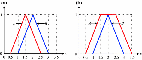

  

  Two type-1 fuzzy sets, A and B, for Exercise 2.44

• (c) Compute $sm_{J} (A,B)$ for the two type-1 fuzzy sets that are depicted in Fig. 2.23b.

• 2.45 Subsethood is also sometimes used in a rule-based fuzzy system, so this exercise explores subsethood for type-1 fuzzy sets. Subsethood is about set containment. Containment is dependent on the order of the two sets, A and B, i.e. A can be contained in B but B does not have to be contained in A, e.g. when $A = \{ 1,2,3\}$ and $B = \{ 1,2,3,4,5,6\}$, $A \subset B$ but $B \not\subset A$. For crisp sets , it is only when $A = B$ that A is contained in B and B is contained in A. For fuzzy sets one knows that everything is a matter of degree; thus, for two type-1 fuzzy sets A and B, it is reasonable to define a degree of subsethood. As usual (in this book), crisp sets are our starting point.

As is stated in Nguyen and Kreinovich (2008): It is known that for two crisp sets A and B: (1) $A \cap B \subseteq A$ and (2) $A \subseteq B$ iff $A \cap B = A$ (create Venn diagrams to convince yourself of the truth of these). So, for crisp sets, to check whether A is a subset of B consider the ratio $|A \cap B|/|A|$ where $| \centerdot |$ denotes the cardinality of $\centerdot$ (see Exercise 2.43 about cardinality). In general this ratio is between 0 and 1, and it equals 1 if and only if A is a subset of B. The smaller the ratio the more there are elements from A which are not part of the intersection $A \cap B$ and thus not part of set B. Consequently, for crisp sets, this ratio can be viewed as a reasonable measure of the degree to which A is a subset of B (see, also, Kosko 1990, 1992).

Because there are many definitions of cardinality for a type-1 fuzzy set as well as the intersection of two type-1 fuzzy sets, there can be many ways to define the subsethood⁴⁰ between two type-1 fuzzy sets. This exercise focuses on what is arguably the most widely used definition of subsethood due to Kosko (1990) and denoted here as $ss_{K} (A,B)$. For a continuous universe of discourse,

$$ ss_{K} (A,B) = \frac{{\int\nolimits_{X} {\hbox{min} (\mu_{A} (x),\mu_{B} (x))dx} }}{{\int\nolimits_{X} {\mu_{A} (x)dx} }} $$

• (a) Explain why $ss_{K} (A,B) \ne ss_{K} (B,A)$.

• (b) What is the formula for $ss_{K} (A,B)$ for discrete universes of discourse?

• (c) Compute $ss_{K} (A,B)$ for the two type-1 fuzzy sets that are depicted in Fig. 2.23a.

• (d) Compute $ss_{K} (A,B)$ for the two type-1 fuzzy sets that are depicted in Fig. 2.23b.

References

Aisbett, J., J.T. Rickard, and D.G. Morgenthaler. 2010. Type-2 fuzzy sets as functions on spaces. IEEE Trans on Fuzzy Systems 18: 841–844.
Allendoerfer, C.B., and C.O. Oakley. 1955. Principles of mathematics. New York: McGraw-Hill.
Arabi, B.N., N. Kehtarnavaz, and C. Lucas. 2001. Restrictions imposed by the fuzzy extension of relations and functions. Journal of Intelligent and Fuzzy Systems 11: 9–22.
Bezdek, J.C. 1981. Pattern recognition with fuzzy objective function algorithms. New York: Plenum.
Bezdek, J., and S.K. Pal. 1992. Fuzzy models for pattern recognition. New York: IEEE Press.
Blanchard, N. 1982. Cardinal and ordinal theories about fuzzy sets. In Fuzzy Information and Decision Process, ed. M. M. Gupta and E. Sanchez, pp. 149–157, Amsterdam.
Bonissone, P. P. and K. S. Decker. 1986. Selecting uncertainty calculi and granularity: An experiment in trading off precision and complexity. In Uncertainty in artificial intelligence, ed. L. N. Kanal and J. F. Lemmer, pp. 217–247, Amsterdam.
Cheeseman, P. 1988. An inquiry into computer understanding. Computational Intelligence 4: 57–142 (with 22 commentaries/replies).
Cox, E.A. 1994. The fuzzy systems handbook. Cambridge, MA: AP Professional.
Cox, E. A. 1992. Fuzzy fundamentals. IEEE Spectrum, pp. 58–61, Oct. 1992.
Dubois, D., and H. Prade. 1980. Fuzzy sets and systems: Theory and applications. NY: Academic Press.
Dubois, D., and H. Prade. 1985. Fuzzy cardinality and the modeling of imprecise quantification. Fuzzy Sets and Systems 16: 199–230.
Dutta, P. H. Boruah and T. Ali. 2011. Fuzzy arithmetic with and without using the α-cut method: A comparative study. International Journal of Latest Trends in Computing 2(1): 99–107 (E-ISSN: 2045-5364).
Edwards, W.F. 1972. Likelihood. London: Cambridge Univ. Press.
Fan, J.L., W.X. Xie, and J. Pei. 1999. Subsethood measure: new definitions. Fuzzy Sets and Systems 106: 201–209.
Gottwald, S. 1980. A note on fuzzy cardinals. Kybernetika 16: 156–158.
He, Q., H.-X. Li, C.L.P. Chen, and E.S. Lee. 2000. Extension principles and fuzzy set categories. Computers and Mathematics with Applications 39: 45–53.
Horikawa, S., T. Furahashi and Y. Uchikawa. 1992. On fuzzy modeling using fuzzy neural networks with back-propagation algorithm. IEEE Transaction on Neural Networks 3: 801–806.
Jaccard, P. 1908. Nouvelles recherches sur la distribution florale. Bulletin de la Societe de Vaud des Sciences Naturelles 44: 223, 1908.
Jang, J.-S.R. 1992. Self-learning fuzzy controllers based on temporal back-propagation. IEEE Transaction on Neural Networks 3: 714–723.
Jang, L.-C., and D. Ralescu. 2001. Cardinality concepts for type-two fuzzy sets. Fuzzy Sets and Systems 118: 479–487.
Jang, J.-S. R., C-T. Sun and E. Mizutani. 1997. Neuro-fuzzy and soft-computing, Prentice-Hall, Upper Saddle River, NJ.
Karnik, N.N., and J.M. Mendel. 2001. Operations on type-2 fuzzy sets. Fuzzy Sets and Systems 122: 327–348.
Karnik, N. N. and J. M. Mendel. 1998. An introduction to type-2 fuzzy logic systems, USC-SIPI Report #418, Univ. of Southern Calif., Los Angeles, CA, June 1998. This can be accessed at: http://sipi.usc.edu/research; then choose “sipi technical reports/418.
Kaufmann, A. 1977. Introduction a la theorie des sous-ensembles flous, complement et nouvelles applications, vol. 4. Paris: Masson.
Klement, E. P. 1982. On the cardinality of fuzzy sets. Proceedings of 6th European meeting on cybernetics and systems research, Vienna, pp. 701–704.
Klir, G.J., and T.A. Folger. 1988. Fuzzy sets, uncertainty, and information. Englewood Cliffs, NJ: Prentice Hall.
Klir, G.J., and B. Yuan. 1995. Fuzzy sets and fuzzy logic: Theory and applications. Upper Saddle River, NJ: Prentice Hall.
Kosko, B. 1990. Fuzziness versus probability. International Journal of General Systems 17: 211–240.
Kosko, B. 1992. Neural network and fuzzy systems, a dynamical systems approach to machine intelligence. Englewood Cliffs, NJ: Prentice-Hall.
Kosko. 1986. Fuzzy entropy and conditioning. Information Sciences 40: 165–174.
Kreinovich, V. 2008. Relations between interval computing and soft computing. In Processing with interval and soft computing, ed. A. de Korvin and V. Kreinovich, 75–97. Springer, London.
Larsen, P. M. 1980. Industrial applications of fuzzy logic control. International Journal Man-Machine Studies 12: 3–10.
Laviolette, M., and J.W. Seaman Jr. 1994. The efficacy of fuzzy representations and uncertainty. IEEE Transaction on Fuzzy Systems 2: 4–15.
Lin, C.-T., and C.S.G. Lee. 1996. Neural fuzzy systems: A neuro-fuzzy synergism to intelligent systems. Upper Saddle River, NJ: Prentice-Hall PTR.
Lindley, B. Y. 1982. Scoring rules and the inevitability of probability. International Statistical Review 50: 1–26 (with 7 commentaries/replies).
De Luca, A., and S. Termini. 1972. A definition of non-probabilistic entropy in the setting of fuzzy sets theory. Information and Computation 20: 301–312.
Macvicar-Whelen, P. J. 1978. Fuzzy sets, the concept of height, and the hedge ‘very’. IEEE Transaction on Systems, Man, and Cybernetics SMC-8: 507–511.
Mamdani, E.H. 1974. Applications of fuzzy algorithms for simple dynamic plant. Proceedings of the IEEE 121: 1585–1588.
Mendel, J.M. 1995a. Fuzzy logic systems for engineering: A tutorial. IEEE Proceedings 83: 345–377.
Mendel, J.M. 1995b. Lessons in estimation theory for signal processing. Prentice-Hall PTR, Englewood Cliffs, NJ: Communications and Control.
Mendel, J.M. 2007. Computing with words: Zadeh, Turing, Popper and Occam. IEEE Computational Intelligence Magazine 2: 10–17.
Mendel, J.M. 2015. Type-2 fuzzy sets and systems: A retrospective. Informatik Spektrum 38 (6): 523–532.
Mendel, J.M., H. Hagras, W.-W. Tan, W.W. Melek, and H. Ying. 2014. Introduction to type-2 fuzzy logic control. Hoboken, NJ: John Wiley and IEEE Press.
Mendel, J.M., and D. Wu. 2010. Perceptual computing: Aiding people in making subjective judgments. Hoboken, NJ: Wiley and IEEE Press.
Nguyen, H.T. 1978. A note on the extension principle for fuzzy sets. Journal of Mathematical Analysis and Applications 64: 369–380.
Nguyen, H. T. and V. Kreinovich. 2008. Computing degrees of subsethood and similarity for interval-valued fuzzy sets: Fast algorithms. In Proceedings of 9th international conference on intelligent technologies in tech’08, pp. 47–55, Samui, Thailand, Oct. 2008.
Rajati, M.R., and J.M. Mendel. 2013. Novel weighted averages versus normalized sums in computing with words. Information Sciences 235: 130–149.
Rudin, W. 1966. Real and complex analysis. New York: Mc-Graw Hill.
Ruspini, E. 1969. A new approach to clustering. Information Control 15: 22–32.
Schmucker, K.S. 1984. Fuzzy set, natural language computations, and risk analysis. Rockville, MD: Computer Science Press.
Wang, L.-X. 1997. A course in fuzzy systems and control. Upper Saddle River, NJ: Prentice-Hall.
Wang, L.-X., and J.M. Mendel. 2016. Fuzzy opinion networks: A mathematical framework for the evolution of opinions and their uncertainties across social networks. IEEE Transaction on Fuzzy Systems 24: 880–905.
Wang, L.-X. and J. M. Mendel. 1992a. Fuzzy basis functions, universal approximation, and orthogonal least squares learning. IEEE Trans. on Neural Networks 3: 807–813.
Wang, L.-X. and J. M. Mendel. 1992b. Back-propagation of fuzzy systems as non-linear dynamic system identifiers. Proceedingas of IEEE intternational conference on fuzzy systems, 1409–1418, San Diego, CA.
Wei, S-H. and S-M. Chen. 2009. Fuzzy risk analysis based on interval-valued fuzzy numbers. Expert Systems with Applications 36: 2285–2299.
Wu, D., and J.M. Mendel. 2007. Uncertainty measures for interval type-2 fuzzy sets. Information Sciences 177: 5378–5393.
Wygralak, M. 1983. A new approach to the fuzzy cardinality of finite fuzzy sets. Busefal 15: 72–75.
Wygralak, M. 2003. Cardinalities of fuzzy sets. Heidelberg: Springer.
Yager, R.R. 1986. A characterization of the fuzzy extension principle. Journal Fuzzy Sets and Systems 18: 205–217.
Yager, R.R., and D.P. Filev. 1994. Essentials of fuzzy modeling and control. New York: Wiley.
Young, V.R. 1996. Fuzzy subsethood. Fuzzy Sets and Systems 77: 371–384.
Zadeh, L.A. 1965. Fuzzy sets. Information and Control 8: 338–353.
Zadeh, L.A. 1971. Similarity relations and fuzzy orderings. Information Sciences 3 (2): 177–200.
Zadeh, L.A. 1972. A fuzzy-set-theoretic interpretation of iinguistic hedges. Journal of Cybernetics 2: 4–34.
Zadeh, L.A. 1981. Possibility theory and soft data analysis. In Mathematical frontiers of the social and policy sciences, ed. L. Cobb, and R.M. Thrall, 69–129. CO: Westview Press, Boulder.
Zadeh, L. A. 1973. Outline of a new approach to the analysis of complex systems and decision processes. IEEE Transaction on Systems, Man, and Cybernetics SMC-3: 28–44.
Zadeh, L. A. 1975. The concept of a linguistic variable and Its application to approximate reasoning–1. Information Sciences 8: 199–249.
Zadeh, L. A. 1999. From computing with numbers to computing with words—from manipulation of measurements to manipulation of perceptions. IEEE Transaction on Circuits and Systems–I: Fundamental Theory and Applications, 4: 105–119.
Zimmermann, H.J. 1991. Fuzzy set theory and its applications, 2nd ed. Boston, MA: Kluwer Academic Publ.
Author information
Authors and Affiliations
Corresponding author