
Abstract
Coupled similarity is a notion of equivalence for systems with internal actions. It has outstanding applications in contexts where internal choices must transparently be distributed in time or space, for example, in process calculi encodings or in action refinements. No tractable algorithms for the computation of coupled similarity have been proposed up to now. Accordingly, there has not been any tool support.
We present a game-theoretic algorithm to compute coupled similarity, running in cubic time and space with respect to the number of states in the input transition system. We show that one cannot hope for much better because deciding the coupled simulation preorder is at least as hard as deciding the weak simulation preorder.
Our results are backed by an Isabelle/HOL formalization, as well as by a parallelized implementation using the Apache Flink framework. Data or code related to this paper is available at: [2].
You have full access to this open access chapter, Download conference paper PDF

1 Introduction
Coupled similarity hits a sweet spot within the linear-time branching-time spectrum [9]. At that spot, one can encode between brands of process calculi [14, 22, 25], name a branching-time semantics for Communicating Sequential Processes [10], distribute synchronizations [23], and refine atomic actions [5, 28]. Weak bisimilarity is too strong for these applications due to the occurrence of situations with partially commited states like in the following example.
Example 1
(Gradually committing philosophers). Three philosophers \(\mathsf {A}\), \(\mathsf {B}\), and \(\mathsf {C}\) want to eat pasta. To do so, they must first sit down on a bench \(\mathrm {s}\) and grab a fork \(\mathrm {f}\). Unfortunately, only either \(\mathsf {A}\) alone or the thinner \(\mathsf {B}\) and \(\mathsf {C}\) together can fit on the bench, and there is just one fork. From the outside, we are only interested in the fact which of them gets to eat. So we consider the whole bench-and-fork business internal to the system. The following \(\mathsf {CCS}\) structure models the situation in the notation of [21]. The resources correspond to output actions (which can be consumed only once) and obtaining the resources corresponds to input actions.

One might now be inclined to ponder that exactly one of the philosophers will get both resources and that we thus could merge \(\mathrm {s}\) and \(\mathrm {f}\) into a single resource \(\mathrm {sf}\):

The structure of \(\mathsf {P}_{g}\) and \(\mathsf {P}_{o}\) has the transition system in Fig. 1 as its semantics. Notice that the internal communication concerning the resource allocation turns into internal \(\tau \)-actions, which in \(\mathsf {P}_{g}\), \(g_{\mathsf {A}}\), and \(g_{\mathsf {BC}}\) gradually decide who is going to eat the pasta, whereas \(\mathsf {P}_{o}\) decides in one step.
\(\mathsf {P}_{g}\) and \(\mathsf {P}_{o}\) are mutually related by a weak simulation (blue dashed lines in Fig. 1) and hence weakly similar. However, there cannot be a symmetric weak simulation relating them because \(\mathsf {P}_g \mathbin {\overset{\tau }{\rightarrow }}g_{\mathsf {BC}}\) cannot be matched symmetrically by \(\mathsf {P}_o\) as no other reachable state shares the weakly enabled actions of \(g_{\mathsf {BC}}\). Thus, they are not weakly bisimilar. This counters the intuition that weak bisimilarity ignores how much internal behavior happens between visible actions. There seems to be no good argument how an outside observer should notice the difference whether an internal choice is made in one or two steps.

A non-maximal weak/coupled simulation  on the philosopher system from Example 1. (Color figure online)

So how to fix this overzealousness of weak bisimilarity? Falling back to weak similarity would be too coarse for many applications because it lacks the property of weak bisimilarity to coincide with strong bisimilarity on systems without internal behavior. This property, however, is present in notions that refine contrasimilarity [31]. There is an easy way to having the cake and eating it, here: Coupled similarity is precisely the intersection of contrasimilarity and weak similarity (Fig. 2). It can be defined by adding a weak form of symmetry (coupling) to weak simulation. The weak simulation in Fig. 1 fulfills coupling and thus is a coupled simulation. This shows that coupled similarity is coarse enough for situations with gradual commitments. At the same time, it is a close fit for weak bisimilarity, with which it coincides for many systems.

Notions of equivalence for systems with internal actions.
Up to now, no algorithms and tools have been developed to enable a wider use of coupled similarity in automated verification settings. Parrow and Sjödin [24] have only hinted at an exponential-space algorithm and formulated as an open research question whether coupled similarity can be decided in \(\mathbf {P}\). For similarity and bisimilarity, polynomial algorithms exist. The best algorithms for weak bisimilarity [3, 19, 26] are slightly sub-cubic in time, \(\mathcal {O}(\vert \mathord {S}\vert ^2 \, \log \vert \mathord {S}\vert )\) for transition systems with \(\vert \mathord {S}\vert \) states. The best algorithms for similarity [15, 27], adapted for weak similarity, are cubic. Such a slope between similarity and bisimilarity is common [18]. As we show, coupled similarity inherits the higher complexity of weak similarity. Still, the closeness to weak bisimilarity can be exploited to speed up computations.
Contributions. This paper makes the following contributions.
-
We prove that action-based single-relation coupled similarity can be defined in terms of coupled delay simulation (Subsect. 2.2).
-
We reduce weak similarity to coupled similarity, thereby showing that deciding coupled similarity inherits the complexity of weak similarity (Subsect. 2.4).
-
We present and verify a simple polynomial-time coupled simulation fixed-point algorithm (Sect. 3).
-
We characterize the coupled simulation preorder by a game and give an algorithm, which runs in cubic time and can be nicely optimized (Sect. 4)
-
We implement the game algorithm for parallel computation using Apache Flink and benchmark its performance (Sect. 5).
Technical details can be found in the first author’s Master’s thesis [1]. Isabelle/HOL [32] proofs are available from https://coupledsim.bbisping.de/isabelle/.
2 Coupled Similarity
This section characterizes the coupled simulation preorder for transition systems with silent steps in terms of coupled delay simulation. We prove properties that are key to the correctness of the following algorithms.
2.1 Transition Systems with Silent Steps
Labeled transition systems capture a discrete world view, where there is a current state and a branching structure of possible state changes (“transitions”) to future states.
Definition 1
(Labeled transition system). A labeled transition system is a tuple \(\mathcal {S}=(S,\varSigma _{\tau },\mathbin {\overset{}{\rightarrow }})\) where S is a set of states, \(\varSigma _{\tau }\) is a set of actions containing a special internal action \(\tau \in \varSigma _{\tau }\), and \(\;\mathbin {\overset{}{\rightarrow }}\subseteq S\times \varSigma _{\tau }\times S\) is the transition relation. We call  the visible actions.
The weak transition relation \(\mathbin {\overset{\hat{\cdot }}{\Rightarrow }}\) is defined as the reflexive transitive closure of internal steps  combined with
  (\(a\in \varSigma \)).
As a shorthand for \(\mathbin {\overset{\hat{\tau }}{\Rightarrow }}\), we also write just \(\mathbin {\overset{}{\Rightarrow }}\). We call an \(\mathbin {\overset{\hat{\alpha }}{\Rightarrow }}\)-step “weak” whereas an \(\mathbin {\overset{\alpha }{\rightarrow }}\)-step is referred to as “strong” (\(\alpha \in \varSigma _{\tau }\)). A visible action \(a\in \varSigma \) is said to be weakly enabled in p iff there is some \(p^{\prime }\) such that \(p\mathbin {\overset{\hat{a}}{\Rightarrow }} p^{\prime }\).
Definition 2
(Stability and divergence). A state p is called stable iff it has no \(\tau \)-transitions,  . A state p is called divergent iff it is possible to perform an infinite sequence of \(\tau \)-transitions beginning in this state, \(p\mathrel {\mathbin {\overset{\tau }{\rightarrow }}^{\omega }}\).
2.2 Defining Coupled Similarity
Coupled simulation is often defined in terms of two weak simulations, but it is more convenient to use just a single one [10], which extends weak simulation with a weak form of symmetry, we shall call coupling (Fig. 3).

Illustration of weak simulation and coupling on transition systems (Definition 4, black part implies red part). (Color figure online)
Definition 3
(Weak simulation). A weak simulation is a relation \(\mathcal {R}\subseteq S\times S\) such that, for all \((p,q)\in \mathcal {R}\), \(p\mathbin {\overset{\alpha }{\rightarrow }}p^{\prime }\) implies that there is a \(q^{\prime }\) such that \(q\mathbin {\overset{\hat{\alpha }}{\Rightarrow }}q^{\prime }\) and \((p^{\prime },q^{\prime })\in \mathcal {R}\).
Definition 4
(Coupled simulation). A coupled simulation is a weak simulation \(\mathcal {R}\subseteq S\times S\) such that, for all \((p,q)\in \mathcal {R}\), there exists a \(q^{\prime }\) such that \(q\mathbin {\overset{}{\Rightarrow }}q^{\prime }\) and \((q^{\prime },p)\in \mathcal {R}\) (coupling).
The coupled simulation preorder relates two processes, \(p\sqsubseteq _{ CS }q\), iff there is a coupled simulation \(\mathcal {R}\) such that \((p,q)\in \mathcal {R}\). Coupled similarity relates two processes, \(p\equiv _{ CS }q\), iff \(p\sqsubseteq _{ CS }q\) and \(q\sqsubseteq _{ CS }p\).
Adapting words from [10], \(p\sqsubseteq _{ CS }q\) intuitively does not only mean that “p is ahead of q” (weak simulation), but also that “q can catch up to p” (coupling). The weak simulation on the philosopher transition system from Example 1 is coupled.
Coupled similarity can also be characterized employing an effectively stronger concept than weak simulation, namely delay simulation. Delay simulations [11, 28] are defined in terms of a “shortened” weak step relation  where
where  and
and  . So the difference between
  and \(\mathbin {\overset{\hat{a}}{\Rightarrow }}\) lies in the fact that the latter can move on with \(\tau \)-steps after the strong \(\mathbin {\overset{a}{\rightarrow }}\)-step in its construction.
Definition 5
(Coupled delay simulation). A coupled delay simulation is a relation \(\mathcal {R}\subseteq S\times S\) such that, for all \((p,q)\in \mathcal {R}\),
-
\(p\mathbin {\overset{\alpha }{\rightarrow }}p^{\prime }\) implies there is a \(q^{\prime }\) such that \(q\) and \((p^{\prime },q^{\prime })\in \mathcal {R}\) (delay simulation),
-
and there exists a \(q^{\prime }\) such that \(q\mathbin {\overset{}{\Rightarrow }}q^{\prime }\) and \((q^{\prime },p)\in \mathcal {R}\) (coupling).
The only difference to Definition 4 is the use of  instead of \(\mathbin {\overset{\hat{\alpha }}{\Rightarrow }}\). Some coupled simulations are no (coupled) delay simulations, for example, consider
  on \(\mathsf {CCS}\) processes. Still, the greatest coupled simulation \(\sqsubseteq _{ CS }\) is a coupled delay simulation, which enables the following characterization:
Lemma 1
\(p\sqsubseteq _{ CS }q\) precisely if there is a coupled delay simulation \(\mathcal {R}\) such that \((p,q)\in \mathcal {R}\).
2.3 Order Properties and Coinduction
Lemma 2
\(\sqsubseteq _{ CS }\) forms a preorder, that is, it is reflexive and transitive. Coupled similarity \(\equiv _{ CS }\) is an equivalence relation.
Lemma 3
The coupled simulation preorder can be characterized coinductively by the rule:

This coinductive characterization motivates the fixed-point algorithm (Sect. 3) and the game characterization (Sect. 4) central to this paper.
Lemma 4
If \(q\mathbin {\overset{}{\Rightarrow }}p\), then \(p\sqsubseteq _{ CS }q\).
Corollary 1
If p and q are on a \(\tau \)-cycle, that means \(p\mathbin {\overset{}{\Rightarrow }}q\) and \(q\mathbin {\overset{}{\Rightarrow }}p\), then \(p\equiv _{ CS }q\).
Ordinary coupled simulation is blind to divergence. In particular, it cannot distinguish two states whose outgoing transitions only differ in an additional \(\tau \)-loop at the second state:
Lemma 5
If \(p \mathbin {\overset{\alpha }{\rightarrow }} p^\prime \longleftrightarrow q \mathbin {\overset{\alpha }{\rightarrow }} p^\prime \vee p^\prime = p \wedge \alpha = \tau \) for all \(\alpha , p^\prime \), then \(p\equiv _{ CS }q\).
Due to the previous two results, finite systems with divergence can be transformed into \(\equiv _{ CS }\)-equivalent systems without divergence. This connects the original notion of stability-coupled similarity [23, 24] to our modern formulation and motivates the usefulness of the next lemma.
Coupling can be thought of as “weak symmetry.” For a relation to be symmetric, \(\mathcal {R}^{-1} \subseteq \mathcal {R}\) must hold whereas coupling means that \(\mathcal {R}^{-1} \subseteq \mathbin {\overset{}{\Rightarrow }} \mathcal {R}\). This weakened symmetry of coupled similarity can guarantee weak bisimulation on steps to stable states:
Lemma 6
Assume \(\mathcal {S}\) is finite and has no \(\tau \)-cycles. Then \(p\sqsubseteq _{ CS }q\) and \(p\mathbin {\overset{\hat{\alpha }}{\Rightarrow }}p^{\prime }\) with stable \(p^{\prime }\) imply there is a stable \(q^{\prime }\) such that \(q\mathbin {\overset{\hat{\alpha }}{\Rightarrow }}q^{\prime }\) and \(p^{\prime }\equiv _{ CS }q^{\prime }\).

Example for \(\mathcal {S}^{\bot }\) from Theorem 1 (\(\mathcal {S}\) in black, \(\mathcal {S}^{\bot }\backslash \mathcal {S}\) in red). (Color figure online)
2.4 Reduction of Weak Simulation to Coupled Simulation
Theorem 1
Every decision algorithm for the coupled simulation preorder in a system \(\mathcal {S}\), \(\sqsubseteq _{ CS }^{\mathcal {S}}\), can be used to decide the weak simulation preorder, \(\sqsubseteq _{ WS }^{\mathcal {S}}\), (without relevant overhead with respect to space or time complexity).
Proof
Let \(\mathcal {S}=(S,\varSigma _{\tau },\mathbin {\overset{}{\rightarrow }})\) be an arbitrary transition system and \(\bot \notin S\). Then

extends \(\mathcal {S}\) with a sink \(\bot \) that can be reached by a \(\tau \)-step from everywhere. For an illustration see Fig. 4. Note that for \(p,q\ne \bot \), \(p\sqsubseteq _{ WS }^{\mathcal {S}}q\) exactly if \(p\sqsubseteq _{ WS }^{\mathcal {S}^{\bot }}q\). On \(\mathcal {S}^{\bot }\), coupled simulation preorder and weak simulation preorder coincide, \(\sqsubseteq _{ WS }^{\mathcal {S}^{\bot }}\,=\,\sqsubseteq _{ CS }^{\mathcal {S}^{\bot }}\), because \(\bot \) is \(\tau \)-reachable everywhere, and, for each p, \(\bot \sqsubseteq _{ CS }^{\mathcal {S}^{\bot }}p\) discharges the coupling constraint of coupled simulation.
Because \(\sqsubseteq _{ WS }^{\mathcal {S}}\) can be decided by deciding \(\sqsubseteq _{ CS }^{\mathcal {S}^{\bot }}\), a decision procedure for \(\sqsubseteq _{ CS }\) also induces a decision procedure for \(\sqsubseteq _{ WS }\). The transformation has linear time in terms of state space size \(\vert \mathord {S}\vert \) and adds only one state to the problem size.
3 Fixed-Point Algorithm for Coupled Similarity
The coinductive characterization of \(\sqsubseteq _{ CS }\) in Lemma 3 induces an extremely simple polynomial-time algorithm to compute the coupled simulation preorder as a greatest fixed point. This section introduces the algorithm and proves its correctness.

3.1 The Algorithm
Roughly speaking, the algorithm first considers the universal relation between states, \(S\times S\), and then proceeds by removing every pair of states from the relation that would contradict the coupling or the simulation property. Its pseudo code is depicted in Algorithm 1.
\(\mathsf {fp\_step}\) plays the role of removing the tuples that would immediately violate the simulation or coupling property from the relation. Of course, such a pruning might invalidate tuples that were not rejected before. Therefore, \(\mathsf {fp\_compute\_cs}\) repeats the process until \(\mathsf {fp\_step}_{\mathcal {S}}(\mathcal {R})=\mathcal {R}\), that is, until \(\mathcal {R}\) is a fixed point of \(\mathsf {fp\_step}_{\mathcal {S}}\).
3.2 Correctness and Complexity
It is quite straight-forward to show that Algorithm 1 indeed computes \(\sqsubseteq _{ CS }\) because of the resemblance between \(\mathsf {fp\_step}\) and the coupled simulation property itself, and because of the monotonicity of \(\mathsf {fp\_step}\).
Lemma 7
If \(\mathcal {R}\) is the greatest fixed point of \(\mathsf {fp\_step}\), then \(\mathcal {R}=\,\sqsubseteq _{ CS }\).
On finite labeled transition systems, that is, with finite S and \(\mathbin {\overset{}{\rightarrow }}\), the while loop of \(\mathsf {fp\_compute\_cs}\) is guaranteed to terminate at the greatest fixed point of \(\mathsf {fp\_step}\) (by a dual variant of the Kleene fixed-point theorem).
Lemma 8
For finite \(\mathcal {S}\), \(\mathsf {fp\_compute\_cs}(\mathcal {S})\) computes the greatest fixed point of \(\mathsf {fp\_step}_{\mathcal {S}}\).
Theorem 2
For finite \(\mathcal {S}\), \(\mathsf {fp\_compute\_cs}(\mathcal {S})\) returns \(\sqsubseteq _{ CS }^{\mathcal {S}}\).
We verified the proof using Isabelle/HOL. Due to its simplicity, we can trust implementations of Algorithm 1 to faithfully return sound and complete \(\sqsubseteq _{ CS }\)-relations. Therefore, we use this algorithm to generate reliable results within test suites for the behavior of other \(\sqsubseteq _{ CS }\)-implementations.
The space complexity, given by the maximal size of \(\mathcal {R}\), clearly is in \(\mathcal {O}(\vert \mathord {S}\vert ^{2})\). Time complexity takes some inspection of the algorithm. For our considerations, we assume that  has been pre-computed, which can slightly increase the space complexity to \(\mathcal {O}(\vert \mathord {\varSigma }\vert \,\vert \mathord {S}\vert ^{2})\).
Lemma 9
The running time of \(\mathsf {fp\_compute\_cs}\) is in \(\mathcal {O}(\vert \mathord {\varSigma }\vert \,\vert \mathord {S}\vert ^{6})\).
Proof
Checking the simulation property for a tuple \((p,q)\in \mathcal {R}\) means that for all \(\mathcal {O}(\vert \mathord {\varSigma }\vert \,\vert \mathord {S}\vert )\) outgoing \(p\mathbin {\overset{\cdot }{\rightarrow }}\)-transitions, each has to be matched by a  -transition with identical action, of which there are at most \(\vert \mathord {S}\vert \). So, simulation checking costs \(\mathcal {O}(\vert \mathord {\varSigma }\vert \,\vert \mathord {S}\vert ^{2})\) time per tuple. Checking the coupling can be approximated by \(\mathcal {O}(\vert \mathord {S}\vert )\) per tuple. Simulation dominates coupling. The amount of tuples that have to be checked is in \(\mathcal {O}(\vert \mathord {S}\vert ^{2})\). Thus, the overall complexity of one invocation of \(\mathsf {fp\_step}\) is in \(\mathcal {O}(\vert \mathord {\varSigma }\vert \,\vert \mathord {S}\vert ^{4})\).
Because every invocation of \(\mathsf {fp\_step}\) decreases the size of \(\mathcal {R}\) or leads to termination, there can be at most \(\mathcal {O}(\vert \mathord {S}\vert ^{2})\) invocations of \(\mathsf {fp\_step}\) in \(\mathsf {fp\_compute\_cs}\). Checking whether \(\mathsf {fp\_step}\) changes \(\mathcal {R}\) can be done without notable overhead. In conclusion, we arrive at an overall time complexity of \(\mathcal {O}(\vert \mathord {\varSigma }\vert \,\vert \mathord {S}\vert ^{6})\).
Now, it does not take much energy to spot that applying the filtering in \(\mathsf {fp\_step}\) to each and every tuple in \(\mathcal {R}\) in every step, would not be necessary. Only after a tuple (p, q) has been removed from \(\mathcal {R}\), the algorithm does really need to find out whether this was the last witness for the \(\exists \)-quantification in the clause of another tuple. While this observation could inspire various improvements, let us fast-forward to the game-theoretic approach in the next section, which elegantly explicates the witness structure of a coupled similarity problem.
4 Game Algorithm for Coupled Similarity
Checking whether two states are related by a (bi-)simulation preorder \(\sqsubseteq _{X}\) can be seen as a game along the lines of coinductive characterizations [30]. One player, the attacker, challenges that \(p\sqsubseteq _{X}q\), while the other player, the defender, has to name witnesses for the existential quantifications of the definition.
Based on the coinductive characterization from Lemma 3, we here define such a game for the coupled simulation preorder and transform it into an algorithm, which basically only amounts to a more clever way of computing the fixed point of the previous section. We show how this additional layer of abstraction enables optimizations.
4.1 The Coupled Simulation Game
The coupled simulation game proceeds as follows: For \(p\sqsubseteq _{ CS }q\), the attacker may question that simulation holds by selecting \(p^{\prime }\) and \(a \in \varSigma \) with \(p\mathbin {\overset{a}{\rightarrow }}p^{\prime }\). The defender then has to name a \(q^{\prime }\) with  , whereupon the attacker may go on to challenge \(p^{\prime }\sqsubseteq _{ CS }q^{\prime }\). If \(p\mathbin {\overset{\tau }{\rightarrow }}p^{\prime }\), the attacker can directly skip to question \(p^{\prime }\sqsubseteq _{ CS }q\). For coupled simulation, the attacker may moreover demand the defender to name a coupling witness \(q^{\prime }\) with \(q\mathbin {\overset{}{\Rightarrow }}q^{\prime }\) whereafter \(q^{\prime }\sqsubseteq _{ CS }p\) stands to question. If the defender runs out of answers, they lose; if the game continues forever, they win. This can be modeled by a simple game, whose schema is given in Fig. 5, as follows.
Definition 6
(Games). A simple game  consists of
-
a (countable) set of game positions G,
-
partitioned into a set of defender positions \(G_{d}\subseteq G\)
-
and attacker positions
 ,
,
-
-
a graph of game moves
 , and
, and -
an initial position \(p_{0}\in G\).
 ,
, , and
, and
Schematic coupled simulation game. Boxes stand for attacker nodes, circles for defender nodes, arrows for moves. From the dashed boxes, the moves are analogous to the ones of the solid box.
Definition 7
(\(\sqsubseteq _{ CS }\) game). For a transition system \(\mathcal {S}=(S,\varSigma _{\tau },\mathbin {\overset{}{\rightarrow }})\), the coupled simulation game  consists of
-
attacker nodes \((p,q)_{\mathtt {a}}\in G_{a}\) with \(p,q\in S\),
-
simulation defender nodes \((a,p,q)_{\mathtt {d}}\in G_{d}\) for situations where a simulation challenge for \(a\in \varSigma \) has been formulated, and
-
coupling defender nodes \((\mathtt {Cpl},p,q)_{\mathtt {d}}\in G_{d}\) when coupling is challenged,
and five kinds of moves
-
simulation challenges
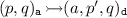 if \(p\mathbin {\overset{a}{\rightarrow }}p^{\prime }\) with \(a \ne \tau \),
 -
simulation internal moves
 if \(p\mathbin {\overset{\tau }{\rightarrow }}p^{\prime }\),
 -
simulation answers
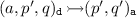 if
if  ,
, -
coupling challenges
 , and
, and -
coupling answers
 if \(q\mathbin {\overset{}{\Rightarrow }}q^{\prime }\).
 if
if  if
if  if
if  ,
, , and
, and if
if Definition 8
(Plays and wins). We call the paths \(p_{0}p_{1}...\in G^{\infty }\) with  plays of \(\mathcal {G}[p_{0}]\). The defender wins all infinite plays. If a finite play \(p_{0}\dots p_{n}\) is stuck, that is, if
  , then the stuck player loses: The defender wins if \(p_{n}\in G_{a}\), and the attacker wins if \(p_{n}\in G_{d}\).
Definition 9
(Strategies and winning strategies). A defender strategy is a (usually partial) mapping from initial play fragments to next moves  . A play p follows a strategy f iff, for each move
  with \(p_{i}\in G_{d}\), \(p_{i+1}=f(p_{0}...p_{i})\). If every such play is won by the defender, f is a winning strategy for the defender. The player with a winning strategy for \(\mathcal {G}[p_{0}]\) is said to win \(\mathcal {G}[p_{0}]\).
Definition 10
(Winning regions and determinacy). The winning region \(W_{\sigma }\) of player \(\sigma \in \{a,d\}\) for a game \(\mathcal {G}\) is the set of states \(p_{0}\) from which player \(\sigma \) wins \(\mathcal {G}[p_{0}]\).
Let us now see that the defender’s winning region of \(\mathcal {G}_{ CS }^{\mathcal {S}}\) indeed corresponds to \(\sqsubseteq _{ CS }^{\mathcal {S}}\). To this end, we first show how to construct winning strategies for the defender from a coupled simulation, and then establish the opposite direction.
Lemma 10
Let \(\mathcal {R}\) be a coupled delay simulation and \((p_{0},q_{0})\in \mathcal {R}\). Then the defender wins \(\mathcal {G}_{ CS }^{\mathcal {S}}[(p_{0},q_{0})_{\mathtt {a}}]\) with the following positional strategy:
-
If the current play fragment ends in a simulation defender node \((a,p^{\prime },q)_{\mathtt {d}}\), move to some attacker node \((p^{\prime },q^{\prime })_{\mathtt {a}}\) with \((p^{\prime },q^{\prime })\in \mathcal {R}\) and
 ;
; -
if the current play fragment ends in a coupling defender node \((\mathtt {Cpl},p,q)_{\mathtt {d}}\), move to some attacker node \((q^{\prime },p)_{\mathtt {a}}\) with \((q^{\prime },p)\in \mathcal {R}\) and \(q\mathbin {\overset{}{\Rightarrow }}q^{\prime }\).
 ;
;Lemma 11
Let f be a winning strategy for the defender in \(\mathcal {G}_{ CS }^{\mathcal {S}}[(p_{0},q_{0})_{\mathtt {a}}]\). Then  is a coupled delay simulation.
Theorem 3
The defender wins \(\mathcal {G}_{ CS }^{\mathcal {S}}[(p,q)_{\mathtt {a}}]\) precisely if \(p\sqsubseteq _{ CS }q\).
4.2 Deciding the Coupled Simulation Game
It is well-known that the winning regions of finite simple games can be computed in linear time. Variants of the standard algorithm for this task can be found in [12] and in our implementation [1]. Intuitively, the algorithm first assumes that the defender wins everywhere and then sets off a chain reaction beginning in defender deadlock nodes, which “turns” all the nodes won by the attacker. The algorithm runs in linear time of the game moves because every node can only turn once.

With such a winning region algorithm for simple games, referred to as \(\mathsf {compute\_winning\_region}\) in the following, it is only a matter of a few lines to determine the coupled simulation preorder for a system \(\mathcal {S}\) as shown in \(\mathsf {game\_compute\_cs}\) in Algorithm 2. One starts by constructing the corresponding game \(\mathcal {G}_{ CS }^{\mathcal {S}}\) using a function \(\mathsf {obtain\_cs\_game}\), we consider given by Definition 7. Then, one calls \(\mathsf {compute\_winning\_region}\) and collects the attacker nodes won by the defender for the result.
Theorem 4
For a finite labeled transition systems \(\mathcal {S}\), \(\mathsf {game\_compute\_cs}(\mathcal {S})\) from Algorithm 2 returns \(\sqsubseteq _{ CS }^{\mathcal {S}}\).
Proof
Theorem 3 states that the defender wins \(\mathcal {G}_{ CS }^{\mathcal {S}}[(p,q)_{\mathtt {a}}]\) exactly if \(p\sqsubseteq _{ CS }^{\mathcal {S}}q\). As \(\mathsf {compute\_winning\_region}(\mathcal {G}_{ CS }^{\mathcal {S}})\), according to [12], returns where the defender wins, line 4 of Algorithm 2 precisely assigns \(\mathcal {R}=\,\sqsubseteq _{ CS }^{\mathcal {S}}\).
The complexity arguments from [12] yield linear complexity for deciding the game by \(\mathsf {compute\_winning\_region}\).
Proposition 1
For a game  , \(\mathsf {compute\_winning\_region}\) runs in
  time and space.
In order to tell the overall complexity of the resulting algorithm, we have to look at the size of \(\mathcal {G}_{ CS }^{\mathcal {S}}\) depending on the size of \(\mathcal {S}\).
Lemma 12
Consider the coupled simulation game  for varying \(\mathcal {S}=(S,\varSigma _{\tau },\mathbin {\overset{}{\rightarrow }})\). The growth of the game size
  is in
is in  .
.
Proof
Let us reexamine Definition 7. There are \(\vert \mathord {S}\vert ^{2}\) attacker nodes. Collectively, they can formulate \(\mathcal {O}(\vert \mathord {\mathbin {\overset{\cdot }{\rightarrow }}}\vert \,\vert \mathord {S}\vert )\) simulation challenges including internal moves and \(\vert \mathord {S}\vert ^{2}\) coupling challenges. There are  simulation answers and \(\mathcal {O}(\vert \mathord {\mathbin {\overset{}{\Rightarrow }}}\vert \,\vert \mathord {S}\vert )\) coupling answers. Of these,
  dominates the others.
Lemma 13
\(\mathsf {game\_compute\_cs}\) runs in  time and space.
Proof
Proposition 1 and Lemma 12 already yield that line 3 is in  time and space. Definition 7 is completely straight-forward, so the complexity of building \(\mathcal {G}_{ CS }^{\mathcal {S}}\) in line 2 equals its output size
  , which coincides with the complexity of computing
  . The filtering in line 4 is in \(\mathcal {O}(\vert \mathord {S}\vert ^{2})\) (upper bound for attacker nodes) and thus does not influence the overall complexity.
4.3 Tackling the \(\tau \)-closure
We have mentioned that there can be some complexity to computing the \(\tau \)-closure \(\mathbin {\overset{}{\Rightarrow }} = \mathbin {\overset{\tau }{\rightarrow }}^{*}\) and the derived  . In theory, both the weak delay transition relation
  and the conventional transition relation \(\mathbin {\overset{\cdot }{\rightarrow }}\) are bounded in size by \(\vert \mathord {\varSigma _{\tau }}\vert \,\vert \mathord {S}\vert ^{2}\). But for most transition systems, the weak step relations tend to be much bigger in size. Sparse \(\mathbin {\overset{\cdot }{\rightarrow }}\)-graphs can generate dense
  -graphs. The computation of the transitive closure also has significant time complexity. Algorithms for transitive closures usually are cubic, even though the theoretical bound is a little lower.
There has been a trend to skip the construction of the transitive closure in the computation of weak forms of bisimulation [3, 13, 19, 26]. With the game approach, we can follow this trend. The transitivity of the game can emulate the transitivity of  (for details see [1, Sec. 4.5.4]). With this trick, the game size, and thus time and space complexity, reduces to \(\mathcal {O}(\vert \mathord {\varSigma _{\tau }}\vert \,\vert \mathord {\mathbin {\overset{\tau }{\rightarrow }}}\vert \,\vert \mathord {S}\vert + \vert \mathord {\mathbin {\overset{\cdot }{\rightarrow }}}\vert \,\vert \mathord {S}\vert )\). Though this is practically better than the bound from Lemma 13, both results amount to cubic complexity \(\mathcal {O}(\vert \mathord {\varSigma }\vert \,\vert \mathord {S}\vert ^{3})\), which is in line with the reduction result from Theorem 1 and the time complexity of existing similarity algorithms.
4.4 Optimizing the Game Algorithm
The game can be downsized tremendously once we take additional over- and under-approximation information into account.
Definition 11
An over-approximation of \(\sqsubseteq _{ CS }\) is a relation \(\mathcal {R}_{O}\) of that we know that \(\sqsubseteq _{ CS }\,\subseteq \mathcal {R}_{O}\). Conversely, an under-approximation of \(\sqsubseteq _{ CS }\) is a relation \(\mathcal {R}_{U}\) where \(\mathcal {R}_{U}\subseteq \,\sqsubseteq _{ CS }\).
Regarding the game, over-approximations tell us where the defender can win, and under-approximations tell us where the attacker is doomed to lose. They can be used to eliminate “boring” parts of the game. Given an over-approximation \(\mathcal {R}_{O}\), when unfolding the game, it only makes sense to add moves from defender nodes to attacker nodes \((p,q)_{\mathtt {a}}\) if \((p,q)\in \mathcal {R}_{O}\). There just is no need to allow the defender moves we already know cannot be winning for them. Given an under-approximation \(\mathcal {R}_{U}\), we can ignore all the outgoing moves of \((p,q)_{\mathtt {a}}\) if \((p,q)\in \mathcal {R}_{U}\). Without moves, \((p,q)_{\mathtt {a}}\) is sure to be won by the defender, which is in line with the claim of the approximation.
Corollary 2
\(\mathbin {\overset{}{\Rightarrow }}^{-1}\) is an under-approximation of \(\sqsubseteq _{ CS }\). (Cf. Lemma 4)
Lemma 14
\(\{(p,q)\!\mid \text {all actions weakly enabled in }p\text { are weakly enabled in }q\}\) is an over-approximation of \(\sqsubseteq _{ CS }\).
The fact that coupled simulation is “almost bisimulation” on steps to stable states in finite systems (Lemma 6) can be used for a comparably cheap and precise over-approximation. The idea is to compute strong bisimilarity for the system  , where maximal weak steps, \(p\mathbin {\mathbin {\overset{\alpha }{\Rightarrow }}\mid }p^{\prime }\), exist iff \(p\mathbin {\overset{\hat{\alpha }}{\Rightarrow }}p^{\prime }\) and \(p^{\prime }\) is stable, that is,
  . Let \(\equiv _{\mathbin {\overset{}{\Rightarrow }}\!\mid }\) be the biggest symmetric relation where \(p\equiv _{\mathbin {\overset{}{\Rightarrow }}\!\mid }q\text { and }p\mathbin {\mathbin {\overset{\alpha }{\Rightarrow }}\mid }p^{\prime }\) implies there is \(q^{\prime }\) such that \(p^{\prime }\equiv _{\mathbin {\overset{}{\Rightarrow }}\!\mid }q^{\prime }\text { and }q\mathbin {\mathbin {\overset{\alpha }{\Rightarrow }}\mid }q^{\prime }.\)
Lemma 15
 is an over-approximation of \(\sqsubseteq _{ CS }\) on finite systems.
Computing \(\equiv _{\mathbin {\overset{}{\Rightarrow }}\!\mid }\) can be expected to be cheaper than computing weak bisimilarity \(\equiv _{ WB }\). After all, \(\mathbin {\mathbin {\overset{\cdot }{\Rightarrow }}\mid }\) is just a subset of \(\mathbin {\overset{\hat{\cdot }}{\Rightarrow }}\). However, filtering \(S\times S\) using subset checks to create  might well be quartic, \(\mathcal {O}(\vert \mathord {S}\vert ^{4})\), or worse. Nevertheless, one can argue that with a reasonable algorithm design and for many real-world examples, \(\mathbin {\mathbin {\overset{\alpha }{\Rightarrow }}\mid }\!\!\equiv _{\mathbin {\overset{}{\Rightarrow }}\!\mid }\) will be sufficiently bounded in branching degree, in order for the over-approximation to do more good than harm.
For everyday system designs,  is a tight approximation of \(\sqsubseteq _{ CS }\). On the philosopher system from Example 1, they even coincide. In some situations,
  degenerates to the shared enabledness relation (Lemma 14), which is to say it becomes comparably useless. One example for this are the systems created by the reduction from weak simulation to coupled simulation in Theorem 1 after \(\tau \)-cycle removal. There, all \(\mathbin {\mathbin {\overset{}{\Rightarrow }}\mid }\)-steps are bound to end in the same one \(\tau \)-sink state \(\bot \).
5 A Scalable Implementation
The experimental results by Ranzato and Tapparo [27] suggest that their simulation algorithm and the algorithm by Henzinger, Henzinger, and Kopke [15] only work on comparably small systems. The necessary data structures quickly consume gigabytes of RAM. So, the bothering question is not so much whether some highly optimized C++-implementation can do the job in milliseconds for small problems, but how to implement the algorithm such that large-scale systems are feasible at all.
To give first answers, we implemented a scalable and distributable prototype of the coupled simulation game algorithm using the stream processing framework Apache Flink [4] and its Gelly graph API, which enable computations on large data sets built around a universal data-flow engine. Our implementation can be found on https://coupledsim.bbisping.de/code/flink/.
5.1 Prototype Implementation
We base our implementation on the game algorithm and optimizations from Sect. 4. The implementation is a vertical prototype in the sense that every feature to get from a transition system to its coupled simulation preorder is present, but there is no big variety of options in the process. The phases are:
-
Import Reads a CSV representation of the transition system \(\mathcal {S}\).
-
Minimize Computes an equivalence relation under-approximating \(\equiv _{ CS }\) on the transition system and builds a quotient system \(\mathcal {S}_{M}\). This stage should at least compress \(\tau \)-cycles if there are any. The default minimization uses a parallelized signature refinement algorithm [20, 33] to compute delay bisimilarity (\(\equiv _{ DB }^{\mathcal {S}}\)).
-
Compute over-approximation Determines an equivalence relation over-approximating \(\equiv _{ CS }^{\mathcal {S}_{M}}\). The result is a mapping \(\sigma \) from states to signatures (sets of colors) such that \(p\sqsubseteq _{ CS }^{\mathcal {S}_{M}}q\) implies \(\sigma (p)\subseteq \sigma (q)\). The prototype uses the maximal weak step equivalence \(\equiv _{\mathbin {\overset{}{\Rightarrow }}\!\mid }\) from Subsect. 4.4.
-
Build game graph Constructs the \(\tau \)-closure-free coupled simulation game \(\mathcal {G}_{ CS }^{\mathcal {S}_{M}}\) for \(\mathcal {S}_{M}\) with attacker states restricted according to the over-approximation signatures \(\sigma \).
-
Compute winning regions Decides for \(\mathcal {G}_{ CS }^{\mathcal {S}_{M}}\) where the attacker has a winning strategy following the scatter-gather scheme [16]. If a game node is discovered to be won by the attacker, it scatters the information to its predecessors. Every game node gathers information on its winning successors. Defender nodes count down their degrees of freedom starting at their game move out-degrees.
-
Output Finally, the results can be output or checked for soundness. The winning regions directly imply \(\sqsubseteq _{ CS }^{\mathcal {S}_{M}}\). The output can be de-minimized to refer to the original system \(\mathcal {S}\).
5.2 Evaluation
Experimental evaluation shows that the approach can cope with the smaller examples of the “Very Large Transition Systems (VLTS) Benchmark Suite” [6] (vasy_* and cwi_* up to 50,000 transitions). On small examples, we also tested that the output matches the return values of the verified fixed-point \(\sqsubseteq _{ CS }\)-algorithm from Sect. 3. These samples include, among others, the philosopher system \(\texttt {phil}\) containing \(\mathsf {P}_{g}\) and \(\mathsf {P}_{o}\) from Example 1 and \(\texttt {ltbts}\), which consists of the finitary separating examples from the linear-time branching-time spectrum [9, p. 73].
Table 1 summarizes the results for some of our test systems with pre-minimization by delay bisimilarity and over-approximation by maximal weak step equivalence. The first two value columns give the system sizes in number of states S and transitions \(\mathbin {\overset{\cdot }{\rightarrow }}\). The next two columns present derived properties, namely an upper estimate of the size of the (weak) delay step relation  , and the number of partitions with respect to delay bisimulation \(S_{/\equiv _{ DB }}\). The next columns list the sizes of the game graphs without and with maximal weak step over-approximation (
 and
and  , some tests without the over-approximation trick ran out of memory, “o.o.m.”). The following columns enumerate the sizes of the resulting coupled simulation preorders represented by the partition relation pair \((S_{/\equiv _{ CS }},\sqsubseteq _{ CS }^{\mathcal {S}_{/\equiv _{ CS }}})\), where \(S_{/\equiv _{ CS }}\) is the partitioning of S with respect to coupled similarity \(\equiv _{ CS }\), and \(\sqsubseteq _{ CS }^{\mathcal {S}_{/\equiv _{ CS }}}\) the coupled simulation preorder projected to this quotient. The last column reports the running time of the programs on an Intel i7-8550U CPU with four threads and 2 GB Java Virtual Machine heap space.
The systems in Table 1 are a superset of the VLTS systems for which Ranzato and Tapparo [27] report their algorithm SA to terminate. Regarding complexity, SA is the best simulation algorithm known. In the [27]-experiments, the C++ implementation ran out of 2 GB RAM for vasy_10_56 and vasy_25_25 but finished much faster than our setup for most smaller examples. Their time advantage on small systems comes as no surprise as the start-up of the whole Apache Flink pipeline induces heavy overhead costs of about 5 s even for tiny examples like phil. However, on bigger examples such as vasy_18_73 their and our implementation both fail. This is in stark contrast to bi-simulation implementations, which usually cope with much larger systems single-handedly [3, 19].
Interestingly, for all tested VLTS systems, the weak bisimilarity quotient system \(S_{/\equiv _{ WB }}\) equals \(S_{/\equiv _{ CS }}\) (and, with the exception of vasy_8_24, \(S_{/\equiv _{ DB }}\)). The preorder \(\sqsubseteq _{ CS }^{\mathcal {S}_{/\equiv _{ CS }}}\) also matches the identity in 6 of 9 examples. This observation about the effective closeness of coupled similarity and weak bisimilarity is two-fold. On the one hand, it brings into question how meaningful coupled similarity is for minimization. After all, it takes a lot of space and time to come up with the output that the cheaper delay bisimilarity already minimized everything that could be minimized. On the other hand, the observation suggests that the considered VLTS samples are based around models that do not need—or maybe even do avoid—the expressive power of weak bisimilarity. This is further evidence for the case from the introduction that coupled similarity has a more sensible level of precision than weak bisimilarity.
6 Conclusion
The core of this paper has been to present a game-based algorithm to compute coupled similarity in cubic time and space. To this end, we have formalized coupled similarity in Isabelle/HOL and merged two previous approaches to defining coupled similarity, namely using single relations with weak symmetry [10] and the relation-pair-based coupled delay simulation from [28], which followed the older tradition of two weak simulations [24, 29]. Our characterization seems to be the most convenient. We used the entailed coinductive characterization to devise a game characterization and an algorithm. Although we could show that deciding coupled similarity is as hard as deciding weak similarity, our Apache Flink implementation is able to exploit the closeness between coupled similarity and weak bisimilarity to at least handle slightly bigger systems than comparable similarity algorithms. Through the application to the VLTS suite, we have established that coupled similarity and weak bisimilarity match for the considered systems. This points back to a line of thought [11] that, for many applications, branching, delay and weak bisimilarity will coincide with coupled similarity. Where they do not, usually coupled similarity or a coarser notion of equivalence is called for. To gain deeper insights in that direction, real-world case studies—and maybe an embedding into existing tool landscapes like FDR [8], CADP [7], or LTSmin [17]—would be necessary.
References
Bisping, B.: Computing coupled similarity. Master’s thesis, Technische Universität Berlin (2018). https://coupledsim.bbisping.de/bisping_computingCoupledSimilarity_thesis.pdf
Bisping, B.: Isabelle/HOL proof and Apache Flink program for TACAS 2019 paper: Computing Coupled Similarity (artifact). Figshare (2019). https://doi.org/10.6084/m9.figshare.7831382.v1
Boulgakov, A., Gibson-Robinson, T., Roscoe, A.W.: Computing maximal weak and other bisimulations. Formal Aspects Comput. 28(3), 381–407 (2016). https://doi.org/10.1007/s00165-016-0366-2
Carbone, P., Katsifodimos, A., Ewen, S., Markl, V., Haridi, S., Tzoumas, K.: Apache Flink: stream and batch processing in a single engine. In: Bulletin of the IEEE Computer Society Technical Committee on Data Engineering, vol. 36, no. 4 (2015)
Derrick, J., Wehrheim, H.: Using coupled simulations in non-atomic refinement. In: Bert, D., Bowen, J.P., King, S., Waldén, M. (eds.) ZB 2003. LNCS, vol. 2651, pp. 127–147. Springer, Heidelberg (2003). https://doi.org/10.1007/3-540-44880-2_10
Garavel, H.: The VLTS benchmark suite (2017). https://doi.org/10.18709/perscido.2017.11.ds100. Jointly created by CWI/SEN2 and INRIA/VASY as a CADP resource
Garavel, H., Lang, F., Mateescu, R., Serwe, W.: CADP 2011: a toolbox for the construction and analysis of distributed processes. Int. J. Softw. Tools Technol. Transfer 15(2), 89–107 (2013). https://doi.org/10.1007/s10009-012-0244-z
Gibson-Robinson, T., Armstrong, P., Boulgakov, A., Roscoe, A.W.: FDR3 — a modern refinement checker for CSP. In: Ábrahám, E., Havelund, K. (eds.) TACAS 2014. LNCS, vol. 8413, pp. 187–201. Springer, Heidelberg (2014). https://doi.org/10.1007/978-3-642-54862-8_13
van Glabbeek, R.J.: The linear time — branching time spectrum II. In: Best, E. (ed.) CONCUR 1993. LNCS, vol. 715, pp. 66–81. Springer, Heidelberg (1993). https://doi.org/10.1007/3-540-57208-2_6
van Glabbeek, R.J.: A branching time model of CSP. In: Gibson-Robinson, T., Hopcroft, P., Lazić, R. (eds.) Concurrency, Security, and Puzzles. LNCS, vol. 10160, pp. 272–293. Springer, Cham (2017). https://doi.org/10.1007/978-3-319-51046-0_14
van Glabbeek, R.J., Weijland, W.P.: Branching time and abstraction in bisimulation semantics. J. ACM (JACM) 43(3), 555–600 (1996). https://doi.org/10.1145/233551.233556
Grädel, E.: Finite model theory and descriptive complexity. In: Grädel, E., et al. (eds.) Finite Model Theory and Its Applications. Texts in Theoretical Computer Science an EATCS Series, pp. 125–130. Springer, Heidelberg (2007). https://doi.org/10.1007/3-540-68804-8_3
Groote, J.F., Jansen, D.N., Keiren, J.J.A., Wijs, A.J.: An \(\cal{O}(m \log n)\) algorithm for computing stuttering equivalence and branching bisimulation. ACM Trans. Comput. Logic (TOCL) 18(2), 13:1–13:34 (2017). https://doi.org/10.1145/3060140
Hatzel, M., Wagner, C., Peters, K., Nestmann, U.: Encoding CSP into CCS. In: Proceedings of the Combined 22th International Workshop on Expressiveness in Concurrency and 12th Workshop on Structural Operational Semantics, and 12th Workshop on Structural Operational Semantics, EXPRESS/SOS, pp. 61–75 (2015). https://doi.org/10.4204/EPTCS.190.5
Henzinger, M.R., Henzinger, T.A., Kopke, P.W.: Computing simulations on finite and infinite graphs. In: 36th Annual Symposium on Foundations of Computer Science, Milwaukee, Wisconsin, pp. 453–462 (1995). https://doi.org/10.1109/SFCS.1995.492576
Kalavri, V., Vlassov, V., Haridi, S.: High-level programming abstractions for distributed graph processing. IEEE Trans. Knowl. Data Eng. 30(2), 305–324 (2018). https://doi.org/10.1109/TKDE.2017.2762294
Kant, G., Laarman, A., Meijer, J., van de Pol, J., Blom, S., van Dijk, T.: LTSmin: high-performance language-independent model checking. In: Baier, C., Tinelli, C. (eds.) TACAS 2015. LNCS, vol. 9035, pp. 692–707. Springer, Heidelberg (2015). https://doi.org/10.1007/978-3-662-46681-0_61
Kučera, A., Mayr, R.: Why is simulation harder than bisimulation? In: Brim, L., Křetínský, M., Kučera, A., Jančar, P. (eds.) CONCUR 2002. LNCS, vol. 2421, pp. 594–609. Springer, Heidelberg (2002). https://doi.org/10.1007/3-540-45694-5_39
Li, W.: Algorithms for computing weak bisimulation equivalence. In: Third IEEE International Symposium on Theoretical Aspects of Software Engineering, 2009. TASE 2009, pp. 241–248. IEEE (2009). https://doi.org/10.1109/TASE.2009.47
Luo, Y., de Lange, Y., Fletcher, G.H.L., De Bra, P., Hidders, J., Wu, Y.: Bisimulation reduction of big graphs on MapReduce. In: Gottlob, G., Grasso, G., Olteanu, D., Schallhart, C. (eds.) BNCOD 2013. LNCS, vol. 7968, pp. 189–203. Springer, Heidelberg (2013). https://doi.org/10.1007/978-3-642-39467-6_18
Milner, R.: Communication and Concurrency. Prentice-Hall Inc., Upper Saddle River (1989)
Nestmann, U., Pierce, B.C.: Decoding choice encodings. Inf. Comput. 163(1), 1–59 (2000). https://doi.org/10.1006/inco.2000.2868
Parrow, J., Sjödin, P.: Multiway synchronization verified with coupled simulation. In: Cleaveland, W.R. (ed.) CONCUR 1992. LNCS, vol. 630, pp. 518–533. Springer, Heidelberg (1992). https://doi.org/10.1007/BFb0084813
Parrow, J., Sjödin, P.: The complete axiomatization of Cs-congruence. In: Enjalbert, P., Mayr, E.W., Wagner, K.W. (eds.) STACS 1994. LNCS, vol. 775, pp. 555–568. Springer, Heidelberg (1994). https://doi.org/10.1007/3-540-57785-8_171
Peters, K., van Glabbeek, R.J.: Analysing and comparing encodability criteria. In: Proceedings of the Combined 22th International Workshop on Expressiveness in Concurrency and 12th Workshop on Structural Operational Semantics, EXPRESS/SOS, pp. 46–60 (2015). https://doi.org/10.4204/EPTCS.190.4
Ranzato, F., Tapparo, F.: Generalizing the Paige-Tarjan algorithm by abstract interpretation. Inf. Comput. 206(5), 620–651 (2008). https://doi.org/10.1016/j.ic.2008.01.001. Special Issue: The 17th International Conference on Concurrency Theory (CONCUR 2006)
Ranzato, F., Tapparo, F.: An efficient simulation algorithm based on abstract interpretation. Inf. Comput. 208(1), 1–22 (2010). https://doi.org/10.1016/j.ic.2009.06.002
Rensink, A.: Action contraction. In: Palamidessi, C. (ed.) CONCUR 2000. LNCS, vol. 1877, pp. 290–305. Springer, Heidelberg (2000). https://doi.org/10.1007/3-540-44618-4_22
Sangiorgi, D.: Introduction to Bisimulation and Coinduction. Cambridge University Press, New York (2012). https://doi.org/10.1017/CBO9780511777110
Stirling, C.: Modal and Temporal Properties of Processes. Springer, New York (2001). https://doi.org/10.1007/978-1-4757-3550-5
Voorhoeve, M., Mauw, S.: Impossible futures and determinism. Inf. Process. Lett. 80(1), 51–58 (2001). https://doi.org/10.1016/S0020-0190(01)00217-4
Wenzel, M.: The Isabelle/Isar Reference Manual (2018). https://isabelle.in.tum.de/dist/Isabelle2018/doc/isar-ref.pdf
Wimmer, R., Herbstritt, M., Hermanns, H., Strampp, K., Becker, B.: Sigref – a symbolic bisimulation tool box. In: Graf, S., Zhang, W. (eds.) ATVA 2006. LNCS, vol. 4218, pp. 477–492. Springer, Heidelberg (2006). https://doi.org/10.1007/11901914_35
Author information
Authors and Affiliations
Corresponding author
Editor information
Editors and Affiliations
Rights and permissions
Open Access This chapter is licensed under the terms of the Creative Commons Attribution 4.0 International License (http://creativecommons.org/licenses/by/4.0/), which permits use, sharing, adaptation, distribution and reproduction in any medium or format, as long as you give appropriate credit to the original author(s) and the source, provide a link to the Creative Commons license and indicate if changes were made.
The images or other third party material in this chapter are included in the chapter's Creative Commons license, unless indicated otherwise in a credit line to the material. If material is not included in the chapter's Creative Commons license and your intended use is not permitted by statutory regulation or exceeds the permitted use, you will need to obtain permission directly from the copyright holder.
Copyright information
© 2019 The Author(s)
About this paper

Cite this paper
Bisping, B., Nestmann, U. (2019). Computing Coupled Similarity. In: Vojnar, T., Zhang, L. (eds) Tools and Algorithms for the Construction and Analysis of Systems. TACAS 2019. Lecture Notes in Computer Science(), vol 11427. Springer, Cham. https://doi.org/10.1007/978-3-030-17462-0_14
Download citation
DOI: https://doi.org/10.1007/978-3-030-17462-0_14
Published:
Publisher Name: Springer, Cham
Print ISBN: 978-3-030-17461-3
Online ISBN: 978-3-030-17462-0
eBook Packages: Computer ScienceComputer Science (R0)
