
Abstract
The extraction of brain tumor tissues in 3D Brain Magnetic Resonance Imaging plays an important role in diagnosis gliomas. In this paper, we use clinical data to develop an approach to segment Enhancing Tumor, Tumor Core, and Whole Tumor which are the sub-regions of glioma. Our proposed method starts with Bit-plane to get the most significant and least significant bits which can cluster and generate more images. Then U-Net, a popular CNN model for object segmentation, is applied to segment all of the glioma regions. In the process, U-Net is implemented by multiple kernels to acquire more accurate results. We evaluated the proposed method with the database BRATS challenge in 2018. On validation data, the method achieves a performance of 82%, 68%, and 70% Dice scores and of 77%, 48%, and 51% on testing data for the Whole Tumor, Enhancing Tumor, and Tumor Core respectively.
You have full access to this open access chapter, Download conference paper PDF
1 Introduction
Accurate extraction of brain tumor types plays an important role in diagnosis and treatment planning. Neuro-imaging methods in Magnetic Resonance Imaging (MRI) provide anatomical and pathophysiological information about brain tumors and aid in diagnosis, treatment planning and follow-up of patients. Manual segmentation of brain tumor tissue is a difficult and time-consuming job. Therefore, brain tumor segmentation from 3D Brain MRI automatically can solve these problems. Among many types of brain tumor, Gliomas are the most common primary brain malignancies, with different degrees of aggressiveness, variable prognosis and various heterogeneous histological sub-regions. In this paper, we focus on Enhancing Tumor, Tumor Core, and Whole Tumor segmentation which are the sub-regions of gliomas segmentation.
Segmentation of brain tumors in multimodal MRI scans is one of the most challenging tasks in medical image analysis. Currently, there are many methods related to brain tumor segmentation have been proposed [1, 2]. In this paper, we divide these methods into two categories: mathematical methods and machine learning methods
-
In mathematical methods: the tumor can be segmented by using threshold, Edge-Based Method [3], Atlas [4]. In Dubey et al. [5], rough set based fuzzy clustering is proposed to segment the tumor.
-
In machine learning methods: Traditionally, many features are extracted manually from image and given to the classifier. However, in recent years, Convolution Neural Networks (CNNs) which have been shown to excel learning a hierarchy task-adapted complex feature are seen prominent success in image classification, object detection and image semantic segmentation [6,7,8]. Many of the brain tumor segmentation methods based on CNNs or combining CNNs with the traditional method are also proposed [9,10,11].
In this study, we combine the Bit-plane method [12] and U-Net architecture [13] for tumor segmentation. First, we use Bit-plane to divide images into many images by determining significant bits. Second, the images with the significant bits can be used to segment the object boundary. Finally, original images and images with least significant bits can be used to determine tissues inside the boundary. Both stages used the U-Net with multiple kernels to segment the tissues more accurately.
The rest of the paper is organized as follows: in the next Sect. 2, we present our proposed method for brain tumor segmentation and the experimental results are shown in Sect. 3. We give the conclusion and discussion in Sect. 4.
2 Our Method
The proposed method is illustrated in Fig. 1. There are three main stages: preprocess, object boundary segmentation, and tissues segmentation. As shown in Fig. 1, after converting to 2D images and grouping images, the first U-Net predicts object boundary of the Whole Tumor and the other U-Net utilizes features to predicts the label of all pixel inside the boundary.

The overall of our proposed method for brain tumor segmentation
2.1 Preprocessing
The preprocessing is the necessary stage before any tissue segmentation. We implement three main steps
-
Normalization: each individual 3D image is scaled to the range [0–255].
-
Brain Slice Category [14]: We group the slices which can contain the tumors together to get the accuracy better. The implementation can be done automatically by learning feature or set manually by omitting some first and end slices. Here, we detect the tumor from slices 40–140.
-
Object Region: each 2D image can be cropped to implement deep learning effectively. Here, we cropped the image size from (256, 256) to (176, 176).
Majority of the volumes in the dataset were acquired along the axial plane and hence had the highest resolution this plane. Therefore, all 3D brain MRI is transformed to 2D brain slices on axial slice extracted from all four sequences. After the preprocessing stage, all the 2D slices is from (155, 256, 256) to (100, 176, 176) with value range (0–255).
2.2 Boundary for All Tumors
The bit plane method [12] is based on decomposing a multilevel image into a series of binary images. The intensities of an image are based on the Eq. (1):
We realize that the final plane contains the most significant bit. In order to segment the boundary of the object, we proposed using k significant bits to eliminate the noise which can affect the image. Instead of using a single plane, we can combine multiple planes together. We represented the slice by keeping from one-bit to eight-bit planes in Fig. 2.

An example of most significant bits from Flair image. In the first row, from the left to the right are images keeping one-bit to four-bit plane. In the second row, from the left to the right are images keeping five-bit to eight-bit plane.
In this study, we eliminate the last 6 bits to remove the noise and only used the first 2 bits to keep the significant data to generate images for training to detect the object boundary. After getting the images, U-Net is used to segment the background and the Whole Tumor by using the 2D slices input and the image which contains 2 significant bits.
2.3 Tissues Segmentation
After segmenting the tumor boundary, different types of tumors inside the boundary can be segmented by using other U-Net. The input data is the data which is preprocessed from the first stage. However, to get a better result, we suggest two contributions to enhance the segmentation:
-
Another training data are the images with noises which are generated from the least significant bits. In this study, we implement the noise from three last bits of each image. The example of the implementation is shown in Fig. 3 with the input from Flair image.
Fig. 3. 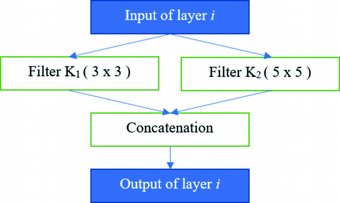
Example using multiple kernels in each convolution for segmentation model
-
Implementing U-Net with multiple kernel size to get the better segmentation [15]. Let \( K = \,\{ (K_{1} ,\,(a_{1} ,\,b_{1} )),\, \ldots \,,\,(K_{n} ,\,(a_{n} \,,\,b_{n} ))\} \) is the set of n filters K with size (a, b). The output of layer i is the merge of feature maps that the layer i generate \( \bigcup\nolimits_{j = 1}^{n} {K_{j} } \). In this study, the numbers within each Conv block comprises of 2 sets of convolutions by 3 × 3 kernels and 2 sets of convolutions by 5 × 5 kernel as shown in Fig. 3.

3 Results
We use BraTS’2018 training data [16,17,18,19], consisting of 210 pre-operative MRI scans of subjects with glioblastoma (HGG) and 75 scans of subjects with lower grade glioma (LGG). These multimodal scans describe (a) native (T1) and (b) post-contrast T1-weighted (T1Gd), (c) T2-weighted (T2), and (d) T2 Fluid Attenuated Inversion Recovery (FLAIR) volumes and were acquired with different clinical protocols and various scanners from multiple (n = 19) institutions. Ground truth annotations comprise the GD-Enhancing Tumor (ET—label 4), the peritumoral edema (ED—label 2), and the necrotic and non-enhancing tumor core (NCR/NET—label 1)
Our proposed method is implemented based on a Keras library [20] with backend Tensorflow [21]. ‘Adam’ optimizer [22] and ‘binary_crossentropy’ loss [23] are used in UNET. We run the method with 50 epochs on Ge-force GTX980 graphics card. Figure 4 shows the result from an example of experiments in the samples of image scans on the real data of the BraTS’18. The top row of Fig. 4 are the original images, from the left to the right: FLAIR, T1, T1ce and T2. The second row contains images from two most significant bits. The third row contains images with noise from three least significant bits. The fourth and the last row is the result of segmentation for each stage.

The results from an example of brain tumor segmentation on the real data of the BraTS’18.
Tables 1 and 2 show the average performance for each label and score for all the validation patients and all the testing patients [24]. The BraTS’18 competition has four metrics to assess the accuracy of segmentation results and to measure the similarity between the segmentations A and B. For the segmentation task, and for consistency with the configuration of the previous BraTS challenges, we will use the Dice score and the Hausdorff distance. Expanding upon this evaluation scheme, BraTS’18 also use the metrics of Sensitivity and Specificity, allowing to determine potential over- or under-segmentations of the tumor sub-regions by participating methods. They are defined as Eqs. (2), (3), (4) and (5)
The Dice metric is the similarity between two volumes A and B, corresponding to the output segmentation of the model and clinical ground truth annotations, respectively. Sensitivity and Specificity are statistical measures employed to evaluate the behavior of the predictions and the proportions of True Positives, False Negatives, False Positives, and True Negatives voxels. Hausdorff(A, B) is the Hausdorff distance between the two surfaces of A and B where \( h\left( {A,B} \right) = max_{a \in A} min_{b \in B} d\left( {a,b} \right) \). Here, \( d\left( {a,b} \right) \) is the Euclidean distance between a and b. This metric indicates the segmentation quality at the border of the tumors by evaluating the greatest distance between the two segmentation surfaces and is independent of the tumor size.
For our participation in BraTS’2018 competition, we used 100% of the training dataset (285 subjects) for training purpose. Our model was trained to segment both HGG and LGG volumes. The result of the proposed method for Enhancing Tumor (ET), Whole Tumor (WT) and Tumor Core (TC) segmentation using the four previously defined metrics are given in Tables 1 and 2. Mean, standard deviation, median are given for Dice and Sensitivity metrics in Table 1 and for Specificity and Hausdorff distance in Table 2. Values presented in Table 1 show high performance on the Dice metric for WT region, but lower performance for ET and TC regions because the noise generating from the Bitplane method has a small difference and is not verified to make it as a real image (Table 3).
4 Conclusions and Discussion
Nowadays, generating data is a good approach for segmentation. In this paper, we propose using Bit-plane to generate more image remaining significant features. Besides, we also implement the U-Net with multiple kernels to get better performance. The result is evaluated without additional data and is shown with a promising performance. In the future, we can concentrate on two main aspects:
-
Using type of image
As shown in Fig. 5, every type of image has specific characteristics. Therefore, instead of using all 4 types of images as an input for all stages, we can use a suitable type of image for each stage to get the better result.
Fig. 5. 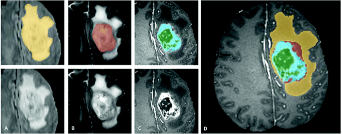
Glioma sub-regions. Shown are image patches with the tumor sub-regions that are annotated in the different modalities (top left) and the final labels for the whole dataset (right). The image patches show from left to right: the Whole Tumor (yellow) visible in T2-FLAIR (Fig. A), the Tumor Core (red) visible in T2 (Fig. B), the Enhancing Tumor structures (light blue) visible in T1Gd, surrounding the cystic/necrotic components of the core (green) (Fig. C). The segmentations are combined to generate the final labels of the tumor sub-regions (Fig. D): edema (yellow), non-enhancing solid core (red), necrotic/cystic core (green), enhancing core (blue) [16,17,18,19]. (Color figure online)
-
Using GAN
Generative Adversarial Networks (GAN) [25] is one of the most promising recent developments in deep learning. GAN solve the problem of unsupervised learning by training two deep networks, called Generator and Discriminator, that compete and cooperate with each other. If we can combine GAN with Bitplane to generate more real images, the result segmentation will be better.

References
Gordillo, N., Montseny, E., Sobrevilla, P.: State of the art survey on MRI brain tumor segmentation. IEEE (2013). https://doi.org/10.1016/j.mri.2013.05.002
Angulakshmi, M., Lakshmi Priya, G.G.: Automated brain tumor segmentation techniques—a review. Int. J. Imaging Syst. Technol. 27, 66–77 (2017). https://doi.org/10.1002/ima.22211
Aslam, A., Khan, E., Beg, M.M.S.: Improved edge detection algorithm for brain tumor segmentation. Procedia Comput. Sci. 58, 430–437 (2015). https://doi.org/10.1016/j.procs.2015.08.057
Bauer, S., Seiler, C., Bardyn, T., Buechler, P., Reyes, M.: Atlas-based segmentation of brain tumor images using a Markov Random Field-based tumor growth model and non-rigid registration. In: Proceedings of IEEE EMBC, pp. 4080–4083 (2010). https://doi.org/10.1109/IEMBS.2010.5627302
Dubey, Y.K., Mushrif, M.M., Mitra, K.: Segmentation of brain MR images using rough set based intuitionistic fuzzy clustering. Biocybern. Biomed. Eng., 413–426 (2016). https://doi.org/10.1016/j.bbe.2016.01.001
Lecun, Y., Bottou, L., Bengio, Y., Haffner, P.: Gradient-based learning applied to document recognition. Proc. IEEE, 2278–2324 (1998). https://doi.org/10.1109/5.726791
Shelhamer, E., Long, J., Darrell, T.: Fully convolutional networks for semantic segmentation. IEEE Trans. Pattern Anal. Mach. Intell. 39(4), 640–651 (2017). https://doi.org/10.1109/CVPR.2015.7298965
Badrinarayanan, V., Kendall, A., Cipolla, R.: SegNet: a deep convolutional en-coder-decoder architecture for image segmentation. IEEE Trans. Pattern Anal. Mach. Intell. 39(12), 2481–2495 (2017). https://doi.org/10.1109/TPAMI.2016.2644615
Guo, L., et al.: A fuzzy feature fusion method for auto-segmentation of gliomas with multimodality diffusion and perfusion magnetic resonance images in radiotherapy. Scientific Reports, vol. 8, Article number: 3231 (2018)
Shukla, G., et al.: Advanced magnetic resonance imaging in glioblastoma: a review. Chin. Clin. Oncol. 6(4), 40 (2017). https://doi.org/10.21037/cco.2017.06.28
Bakas, S., et al.: GLISTRboost: combining multimodal MRI segmentation, registration, and biophysical tumor growth modeling with gradient boosting machines for glioma segmentation. In: Crimi, A., Menze, B., Maier, O., Reyes, M., Handels, H. (eds.) BrainLes 2015. LNCS, vol. 9556, pp. 144–155. Springer, Cham (2016). https://doi.org/10.1007/978-3-319-30858-6_13
Gonzalez, R.C., Woods, R.E.: Digital Image Processing. Prentice Hall Inc., Upper Saddle River (2002)
Ronneberger, O., Fischer, P., Brox, T.: U-Net: convolutional networks for biomedical image segmentation. In: Navab, N., Hornegger, J., Wells, W.M., Frangi, A.F. (eds.) MICCAI 2015. LNCS, vol. 9351, pp. 234–241. Springer, Cham (2015). https://doi.org/10.1007/978-3-319-24574-4_28
Tuan, T.A., Kim, J.Y., Bao, P.T.: 3D brain magnetic resonance imaging segmentation by using bitplane and adaptive fast marching. Int. J. Imaging Syst. Technol. 28, 223–230 (2018). https://doi.org/10.1002/ima.22273
Szegedy, C., et al.: Going deeper with convolutions. In: IEEE Conference on Computer Vision and Pattern Recognition (CVPR) (2015). https://doi.org/10.1109/CVPR.2015.7298594
Menze, B.H., et al.: The multimodal brain tumor image segmentation benchmark (BRATS). IEEE Trans. Med. Imaging 34(10), 1993–2024 (2015). https://doi.org/10.1109/TMI.2014.2377694
Bakas, S., et al.: Advancing The Cancer Genome Atlas glioma MRI collections with expert segmentation labels and radiomic features. Nat. Sci. Data 4, 170117 (2017). https://doi.org/10.1038/sdata.2017.117
Bakas, S., et al.: Segmentation labels and radiomic features for the pre-operative scans of the TCGA-GBM collection. The Cancer Imaging Archive (2017). https://doi.org/10.7937/k9/TCIA.2017.KLXWJJ1Q
Bakas, S., et al.: Segmentation labels and radiomic features for the pre-operative scans of the TCGA-LGG collection. The Cancer Imaging Archive (2017). https://doi.org/10.7937/K9/TCIA.2017.GJQ7R0EF
Chollet, F., et al.: Keras (2015). https://keras.io
Abadi, M., et al.: TensorFlow: a system for large-scale machine learning. In: OSDI, vol. 16, pp. 265–283 (2016)
Kingma, D.P., Ba, L.J.: Adam: a method for stochastic optimization. In: International Conference on Learning Representations (2015)
Bishop, C.M.: Pattern Recognition and Machine Learning. Springer, New York (2006)
Bakas, S., Reyes, M., et al.: Identifying the best machine learning algorithms for brain tumor segmentation, progression assessment, and overall survival prediction in the BRATS challenge. arXiv preprint arXiv:1811.02629 (2018)
Goodfellow, I.J., et al.: Generative adversarial nets. In: Proceedings of the 27th International Conference on Neural Information Processing Systems, NIPS 2014 (2014)
Acknowledgement
We would like to thank Business Intelligence LAB at University of Economics and Law for supporting us throughout this paper. The study was supported by Science and Technology Incubator Youth Program, managed by the Center for Science and Technology Development, Ho Chi Minh Communist Youth Union, 2018.
Author information
Authors and Affiliations
Corresponding author
Editor information
Editors and Affiliations
Rights and permissions
Copyright information
© 2019 Springer Nature Switzerland AG
About this paper

Cite this paper
Tuan, T.A., Tuan, T.A., Bao, P.T. (2019). Brain Tumor Segmentation Using Bit-plane and UNET. In: Crimi, A., Bakas, S., Kuijf, H., Keyvan, F., Reyes, M., van Walsum, T. (eds) Brainlesion: Glioma, Multiple Sclerosis, Stroke and Traumatic Brain Injuries. BrainLes 2018. Lecture Notes in Computer Science(), vol 11384. Springer, Cham. https://doi.org/10.1007/978-3-030-11726-9_41
Download citation
DOI: https://doi.org/10.1007/978-3-030-11726-9_41
Published:
Publisher Name: Springer, Cham
Print ISBN: 978-3-030-11725-2
Online ISBN: 978-3-030-11726-9
eBook Packages: Computer ScienceComputer Science (R0)