
Abstract
We present an inversion scheme to recover the (1-D) depth profile of mantle conductivity from satellite magnetic data, which takes into account 3-D effects arising from the distribution of oceans and continents. The scheme is based on an iterative inversion of C-responses, which are estimated from time series of the dominating external (inducing) and internal (induced) spherical harmonic coefficients of the magnetic potential due to a magnetospheric source. These time series will be available as a Swarm Level-2 data product. We verify our approach by using synthetic, but realistic time series obtained by simulating induction due to a realistic magnetospheric source in a 3-D “target” conductivity model of the Earth. This model contains not only a laterally heterogeneous layer representing oceans and continents, but also 3-D inhomogeneities in the mantle. The inversion for mantle conductivity is initiated with a uniform conductivity model. Convergence is reached within a few iterations. The recovered model agrees well with the laterally averaged target model, although the latter comprises large jumps in conductivity. Our 1-D inversion scheme is therefore ready to process Swarm data.
1. Introduction
Temporal variations of Earth’s magnetic field have long been used to infer global 1-D conductivity profiles of Earth’s mantle, mostly from continental geomagnetic observatories (e.g. Schmucker, 1985; Schultz and Larsen, 1987; Olsen, 1998). In contrast to data from observatories, which are sparse and irregularly distributed (with only few in oceanic regions), data of uniform quality with a good spatial coverage can be obtained from low-Earth-orbit (LEO) platforms. This enables the derivation of a globally-averaged conductivity profile that is not biased towards continental regions.
However, analysis of satellite data is more challenging compared to analysis of observatory data for two reasons: First, LEO satellites move typically with a speed of 7–8 km/s and thus measure a mixture of temporal and spatial changes of the magnetic field. Second, satellites pass over both continents and oceans, and therefore the magnetic satellite data are affected by induction in the oceans (cf. Tarits and Grammatica, 2000; Everett et al., 2003; Kuvshinov and Olsen, 2005) in a complicated way. In spite of these difficulties, a number of attempts has been made to probe mantle conductivity from space (e.g. Didwall, 1984; Olsen, 1999; Olsen et al., 2002; Constable and Constable, 2004; Velímský et al., 2006). Most recently, Kuvshinov and Olsen (2006) derived a global model of mantle conductivity from five years of CHAMP, Ørsted and SAC-C magnetic data and demonstrated the necessity of taking into account the contributions of a laterally heterogeneous surface shell representing the distribution of oceans and continents. The authors accounted for the ocean effect by correcting the magnetic field at orbit altitudes.
As in the paper by Kuvshinov and Olsen (2006), we present in this paper a methodology to determine the 1-D conductivity profile of Earth’s mantle by inverting global C-responses. These are estimated from time series of the dominating external (inducing) and internal (induced) spherical harmonic expansion (SHE) coefficients of the magnetic potential that describes the signals of magnetospheric origin. Both time series will be available as Swarm Level-2 data product MMA SHA 2, determined by the Comprehensive Inversion chain (CI, Sabaka et al., 2013) of the Swarm Level-2 Processing Facility SCARF (Olsen et al., 2013). The CI aims to separate magnetic contributions from various sources (originating in the core, lithosphere, ionosphere and magnetosphere) in the form of corresponding SHE coefficients. As Kuvshinov and Olsen (2006), we also correct for the ocean effect, but our correction scheme differs from that presented by the authors in two aspects. First, our scheme is iterative, i.e. a correction for the ocean effect is applied multiple times. Second, we do not make the detour of predicting the magnetic field at orbit altitudes, but directly correct the estimated C-responses.
In Section 2 of this paper, we outline the inversion algorithm and describe how we account for the ocean effect. Section 3 presents results of a model study. We summarize our work in Section 4.
2. Inversion Algorithm
In this section, we outline the succession of processing steps that forms the inversion scheme. A summary is presented in Fig. 1. Note that our inversion scheme is iterative. The iterative structure is due to the applied correction for the ocean effect (arising from a laterally heterogeneous surface shell). Without accounting for this effect, only the estimate of global C -responses from the observed data (Subsection 2.1) and the subsequent recovery of a conductivity model (Subsection 2.3) would be necessary. However, the C -responses estimated in such a way would be biased at short periods, thus also biasing the recovered conductivity model (mainly at shallow depths, cf. Kuvshinov and Olsen, 2006).

Scheme of the processing steps (yellow boxes) that constitute the iterative 1-D inversion. Inputs are marked by grey boxes, outputs by orange boxes. Note that by the term “3-D model”, we denote the 1-D model plus a laterally heterogeneous surface shell.
2.1 Estimation of global C-responses
In the source-free region above the conducting Earth, the magnetic field due to a magnetospheric source can be represented as gradient of a scalar potential, B = − ∇ V, which is obtained by solving Laplace’s equation. The potential V can be expanded into external and internal spherical harmonic sources. We assume a ring current geometry for the external part of V, described by a single spherical harmonic coefficient,  . In a 1-D Earth, a source with this geometry only induces one internal coefficient,
  . Thus, V can (in frequency domain) be written as

where ϑ denotes colatitude, r denotes distance from Earth’s centre, a is Earth’s mean radius and ω is angular frequency. The 1-D electromagnetic transfer function of degree 1, Q1 (ω), is defined by the relation

Time series of  and
and  , provided by the CI, are the inputs for our inversion. We use the section averaging approach (Olsen, 1998) and a robust statistical procedure involving iteratively re-weighted least squares (Aster et al, 2005) to estimate the transfer function
  (and the corresponding uncertainties
  from
from  and
and  at a set of (logarithmically spaced) frequencies ω. The 1-D Q-response is transformed to the global C -response by means of

with corresponding errors

which follows from the error propagation law.
2.2 Correction of estimated C-responses
Within each iteration of the inversion scheme, we simulate induction in a 1-D model and a 3-D model, yielding the synthetic global C-responses C1-D(ω) and C3-D(ω), respectively (cf. Fig. 1). The 1-D model consists of the 1-D conductivity structure recovered in the previous iteration of the inversion. With the term “3-D model”, we denote this 1-D model plus a laterally heterogeneous surface shell. The calculation of synthetic C-responses for a X-D model, where X-D refers to either 1-D or 3-D, involves three steps:
-
1)
Calculation of BX-D,unit(r = a, ϑ, φ,ω), i.e. the magnetic field at Earth’s surface due to a unit amplitude magnetospheric ring current source at a set of frequencies ω. Note that the calculated magnetic field only varies in longitude φ if the model contains 3-D heterogeneities.
-
2)
Recovery of the transfer function
 by spherical harmonic analysis of
  using the formula
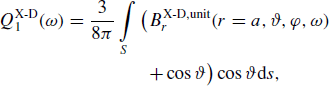 (5)
(5)where ds = sinϑdϑdφ. Equation (5) follows from B = −∇V with V given by Eq. (1), the definition of the Q-response (2) and
 .
. -
3)
Transformation of
 to CX-D(ω) using Eq. (3).
 by spherical harmonic analysis of
  using the formula
 .
. to CX-D(ω) using
 To compute the magnetic field in a 3-D conductivity model (item 1 of the above list), we use a 3-D contracting integral equation solver, extensively described in Kuvshinov and Semenov (2012).
We correct the global C-responses estimated from observed data, Cobs(ω) (cf. Subsection 2.1), for the ocean effect with the formula

This correction diminishes 3-D effects (arising from the laterally heterogeneous surface shell) in the data. If our 3-D conductivity model coincides with the true conductivity structure of the Earth, C3-D(ω) and Cobs(ω) cancel out except for measurement errors, and Ccorr(ω) is then simply given by C1-D(ω). This logic is also applied to decide when to stop iterating. Convergence of the iterative scheme is reached if the weighted RMS of Cobs(ω) and C3-D(ω) falls below a prescribed threshold ϵ, i.e. if

where N ω is the number of periods at which responses were estimated. If, on the other hand, the RMS is larger than ϵ, the corrected C -responses are inverted for a new 1-D conductivity model, and a new iteration is initiated (cf. Fig. 1).
2.3 Derivation of the 1-D conductivity model
We derive the 1-D conductivity model from the corrected C -responses Ccorr(ω) by using the quasi-Newton algorithm of Byrd et al. (1995). The inversion is stabilized by minimizing the first derivative of log(conductivity) with respect to log(depth). Inversion is performed for several regular-ization parameters (i.e. several degrees of smoothing). The solution is picked from a trade-off curve (L-curve), which relates data misfit and model complexity (Hansen, 1992).
3. Model Study
In order to test the performance of our inversion scheme, we generate synthetic data (i.e. time series of induced coefficients) in a test 3-D conductivity model, hereinafter referred to as “target model”, and afterwards recover the 1-D conductivity structure of the target model (i.e. its laterally averaged conductivity) from the data. We introduce the target conductivity model (Subsection 3.1), describe how we generate the test data (Subsection 3.2) and finally present the results of our model study (Subsection 3.3).
3.1 Target conductivity model
Figure 2 shows the target conductivity model. It consists of a thin surface shell of laterally varying conductance and a layered model, which contains different conductivity anomalies, underneath. The surface shell is scaled to a thickness of 10 km. The conductivity anomalies in deeper regions are introduced in order to simulate that the true Earth most probably also contains 3-D mantle heterogeneities. Also note that the same target model has been used in the associated 3-D mantle conductivity inversion studies (cf. companion papers by Puthe and Kuvshinov, 2013; Velímský, 2013).

Target conductivity model used in our model study, units are in S/m. Note that the conductivity of the top layer has been obtained by scaling the surface conductance map to a thickness of 10 km.
3.2 Generation of the test data set
Hourly mean time series of external SHE coefficients in a geomagnetic dipole coordinate system (up to degree 3 and order 1) have been derived by analysis of 4.5 years of observatory data (July 1998-December 2002), details of the derivation are given in Olsen et al. (2005). Time series of internal SHE coefficients are synthesized by simulating induction in the target conductivity model (Subsection 3.1), cf. companion paper by Puthe and Kuvshinov (2013).
We use the time series of external and internal coefficients to predict the magnetospheric field at orbit altitudes (with a sampling frequency of 1 Hz). Adding the contributions due to different sources (core, lithosphere and ionosphere) yields the magnetic field at orbit altitudes, which is then analyzed by the CI. The external and internal SHE coefficients of the magnetic potential due to magnetospheric sources recovered by the CI constitute a realistic test data set for our inversion scheme. A more detailed description of the generation of the test data set is provided in Olsen et al. (2013).
3.3 Inversion results
Recovered time series of  and
and  are provided by the CI with a sampling rate of 1.5 hours (Level-2 data product MMA_SHA_2_, cf. Sabaka et al., 2013). The time series are depicted in Fig. 3. With these data, we estimate C-responses at 23 logarithmically spaced periods between 14 hours and 83 days. We invert the C -responses to recover the 1-D mantle conductivity at depths between 10 km and the core-mantle boundary at 2890 km. The inversion domain is stratified into in total 44 layers with thicknesses of 50 km (at depths below 1500 km) and 100 km (at depths greater than 1500 km), respectively. As initial (starting) model, a uniform mantle with conductivity of 1 S/m is prescribed.

Input data of the model study–time series of  and
and  (in nT). The time (in days) is relative to January 1, 2000. Note that the time series of
  has been shifted by 150 nT for clarity.
For a chosen threshold value ϵ = 5 (cf. Eq. (7)), the inversion scheme converged after 5 iterations. Figure 4 shows the convergence of the C-responses. The recovered conductivity model in comparison to the (laterally averaged) target model is shown in Fig. 5. Lateral averaged conductivity here denotes the arithmetic mean of the conductivity of all cells in the respective layer. The results indicate that the inversion scheme is able to accurately recover mantle conductivity at all depths. Although the conductivity of the initial model is very different from the target conductivity structure, the final model agrees well with the target model. Due to the applied smoothing, the recovered model does not comprise the large jumps in conductivity that are apparent in the target model at depths of 400 km and 700 km. Such large jumps in conductivity are, however, not likely for true Earth.

Demonstration of the convergence of observed global C-responses Cobs(ω) and C-responses calculated in the current 3-D model, C3-D(ω), within five iterations of the inversion scheme. Note that the series with positive values correspond to Re C, those with negative values to Im C.

Recovered conductivity model (blue) in comparison to the uniform initial model (green) and the laterally averaged target conductivity model (red; compare with Fig. 2). Note that the conductivity of the core is fixed to 105 S/m.
4. Conclusions
We have presented a scheme to invert satellite magnetic data for a global depth profile of mantle conductivity. The scheme is based on the inversion of C-responses and comprises a correction for the ocean effect. In spite of the iterative architecture and a number of processing steps, final results can be obtained within a few hours. The repeated calculation of the magnetic field in a 3-D model is the most expensive step in terms of computational cost.
The algorithm has been tested by simulating induction due to a realistic magnetospheric source in a realistic 3-D (target) conductivity model and recovering the 1-D conductivity structure of this model (i.e. its laterally averaged conductivity) from the synthetic data. In spite of large conductivity jumps and a number of 3-D heterogeneities in the target model, an excellent recovery of the 1-D conductivity of Earth’s mantle has been achieved from crustal depths to the core-mantle boundary. The algorithm has thus proved to be workable and ready to digest Swarm data. Moreover, the inversion results provide a useful initial guess for 3-D mantle conductivity studies with Swarm data (cf. companion papers by Puthe and Kuvshinov, 2013; Velímský, 2013).
References
Aster, R. C, B. Borchers, and C. H. Thurber, Parameter Estimation and Inverse Problems, Elsevier Academic Press, Burlington, U.S.A., 2005.
Byrd, R., P. Lu, J. Nocedal, and C. Zhu, A limited memory algorithm for bound constrained optimization, SIAM J. Sci. Comput., 5, 1190–1208, 1995.
Constable, S. and C. Constable, Observing geomagnetic induction in magnetic satellite measurements and associated implications for mantle conductivity, Geochem. Geophys. Geosyst., 5, doi:10.1029/2003GC000634, 2004.
Didwall, E., The electrical conductivity of the upper mantle as estimated from satellite magnetic field data, J. Geophys. Res., 89, 537–542, 1984.
Everett, M. E., S. Constable, and C. G. Constable, Effects of near-surface conductance on global satellite induction responses, Geophys. J. Int., 153, 277–286, 2003.
Hansen, P. C, Analysis of discrete ill-posed problems by means of the L-curve, SIAMRev., 34, 561–580, 1992.
Kuvshinov, A. and N. Olsen, Modelling the ocean effect of geomagnetic storms at ground and satellite altitude, in Earth Observation with CHAMP. Results from Three Years in Orbit, edited by Ch. Reigber, H. Lühr, P. Schwintzer, and J. Wickert, pp. 353–358, Springer-Verlag, Berlin Heidelberg, 2005.
Kuvshinov, A. and N. Olsen, A global model of mantle conductivity derived from 5 years of CHAMP, Ørsted, and SAC-C magnetic data, Geophys. Res. Lett., 33, doi:10.1029/2006GL027083, 2006.
Kuvshinov, A. and A. Semenov, Global 3-D imaging of mantle electrical conductivity based on inversion of observatory C-responses I. An approach and its verification, Geophys.J.Int., 189, doi:10.1111/j.1365-246X.2011.05349.x, 2012.
Olsen, N., The electrical conductivity of the mantle beneath Europe derived from C-responses from 3 to 720 hr, Geophys. J. Int., 133, 298–308, 1998.
Olsen, N., Long-period (30 days-1 year) electromagnetic sounding and the electrical conductivity of the lower mantle beneath Europe, Geophys. J. Int., 138, 179–187, 1999.
Olsen, N., S. Vennerstrøm, and E. Friis-Christensen, Monitoring magneto-spheric contributions using ground-based and satellite magnetic data, in First CHAMP Mission Results for Gravity, Magnetic and Atmospheric Studies, edited by Ch. Reigber, H. Lühr, and P. Schwintzer, pp. 245–250, Springer-Verlag, Berlin Heidelberg, 2002.
Olsen, N., F. Lowes, and T. Sabaka, Ionospheric and induced field leakage in geomagnetic field models, and derivation of candidate models for DGRF 1995 and DGRF 2000, Earth Planets Space, 57, 1191–1196, 2005.
Olsen, N., E. Friis-Christensen, R. Floberghagen, P. Alken, C. D Beggan, A. Chulliat, E. Doornbos, J. T. da Encarnação, B. Hamilton, G. Hulot, J. van den IJssel, A. Kuvshinov, V. Lesur, H. Luhr, S. Macmillan, S. Maus, M. Noja, P. E. H. Olsen, J. Park, G. Plank, C. Puthe, J. Rauberg, P. Rit-ter, M. Rother, T. J. Sabaka, R. Schachtschneider, O. Sirol, C. Stolle, E. Thébault, A. W. P. Thomson, L. Tøffner-Clausen, J. Velímský, P. Vi-gneron, and P. N. Visser, The Swarm Satellite Constellation Application and Research Facility (SCARF) and Swarm data products, Earth Planets Space, 65, this issue, 1189–1200, 2013.
Puthe, C. and A. Kuvshinov, Determination of the 3-D distribution of electrical conductivity in Earth’s mantle from Swarm satellite data: Frequency domain approach based on inversion of induced coefficients, Earth Planets Space, 65, this issue, 1247–1256, 2013.
Sabaka, T. J., L. Tøffner-Clausen, and N. Olsen, Use of the Comprehensive Inversion method for Swarm satellite data analysis, Earth Planets Space, 65, this issue, 1201–1222, 2013.
Schmucker, U., Electrical properties of the Earth’s interior, Landolt-Bornstein, New Series, 5/2b, pp. 370–397, Springer-Verlag, Berlin Heidelberg, 1985.
Schultz, A. and J. C. Larsen, On the electrical conductivity of the mid-mantle: I Calculation of equivalent scalar magnetotelluric response functions, Geophys. J. Int., 88(3), 733–761, 1987.
Tarits, P. and N. Grammatica, Electromagnetic induction effects by the solar quiet magnetic field at satellite altitude, Geophys. Res. Lett., 27, 4009–4012, 2000.
Velimsky, J., Determination of three-dimensional distribution of electrical conductivity in the Earth’s mantle from Swarm satellite data: Time-domain approach, Earth Planets Space, 65, this issue, 1239–1246,2013.
Velímský, J., Z. Martinec, and M. E. Everett, Electrical conductivity in the Earth’s mantle inferred from CHAMP satellite measurements—I. Data processing and 1-D inversion, Geophys. J. Int., 166, 529–542, 2006.
Acknowledgments
The authors thank Nils Olsen for a careful and constructive review of the manuscript. This work has been supported by the European Space Agency through ESTEC contract No. 4000102140/10/NL/JA, by the Swiss National Science Foundation under grant No. 2000021-140711/1, and in part by the Russian Foundation for Basic Research under grant No. 12-05-00817-a.
Author information
Authors and Affiliations
Corresponding author
Rights and permissions
Open Access This article is licensed under a Creative Commons Attribution 4.0 International License, which permits use, sharing, adaptation, distribution and reproduction in any medium or format, as long as you give appropriate credit to the original author(s) and the source, provide a link to the Creative Commons licence, and indicate if changes were made.
The images or other third party material in this article are included in the article’s Creative Commons licence, unless indicated otherwise in a credit line to the material. If material is not included in the article’s Creative Commons licence and your intended use is not permitted by statutory regulation or exceeds the permitted use, you will need to obtain permission directly from the copyright holder.
To view a copy of this licence, visit https://creativecommons.org/licenses/by/4.0/.
About this article
Cite this article
Püthe, C., Kuvshinov, A. Determination of the 1-D distribution of electrical conductivity in Earth’s mantle from Swarm satellite data. Earth Planet Sp 65, 1233–1237 (2013). https://doi.org/10.5047/eps.2013.07.007
Received:
Revised:
Accepted:
Published:
Issue Date:
DOI: https://doi.org/10.5047/eps.2013.07.007