
Abstract
In this review we give an overview about the current state-of-knowledge of the magnetic field in sunspots from an observational point of view. We start by offering a brief description of tools that are most commonly employed to infer the magnetic field in the solar atmosphere with emphasis in the photosphere of sunspots. We then address separately the global and local magnetic structure of sunspots, focusing on the implications of the current observations for the different sunspots models, energy transport mechanisms, extrapolations of the magnetic field towards the corona, and other issues.
1 Introduction
1.1 Role of magnetic field in cosmic bodies
The role of the magnetic field has become firmly recognized in astrophysics as humans discover the rich variety of phenomena present in the universe. The largest constituent of cosmic bodies is in the state of plasma, i.e., ionized gas, which interacts with magnetic fields. Through this interaction the magnetic field is responsible for many of the structures and dynamics that we observe with modern instrumentation. The fundamental role of magnetic fields can be summarized as follows:
-
By trapping charged particles, the magnetic field guides the plasma motions (for example, it confines plasma or suppresses the convective fluid motions) and generates a variety of density structures in universe.
-
The magnetic pressure causes the plasma to expand and makes it buoyant, thereby driving the emergence of magnetic loops into the tenuous ‘outer’ atmosphere against the action of gravity.
-
The magnetic field guides (MHD) waves and transports energy and disturbances from a site of energy injection to other locations.
-
Magnetic fields inhibit the thermal conduction across them, and make the presence of multitemperature structures possible in tenuous, high conductivity gas like stellar corona.
-
The magnetic field stores and releases energy that produces transient dynamic phenomena like flare explosions and plasma ejections.
-
The magnetic field also plays a crucial role in accelerating non-thermal particles to the relativistic regime in tenuous plasmas.
The magnetic field is, therefore, one of the fundamental ingredients of the universe. In the case of the Sun, our nearest star, we observe spectacular active and dynamic phenomena driven by magnetic fields with their spatial, temporal, and spectral structures in detail. Because of this, the Sun serves as an excellent plasma laboratory and provides us a unique opportunity to study the fundamental processes of the cosmical magnetohydrodynamics. Let us make an addition on the list of the role of the magnetic field, i.e.:
-
The magnetic field produces or modifies the polarization property of the light emitted from, or absorbed by, cosmical bodies, making themselves measurable.
1.2 Discovery of sunspot’s magnetic field
The key physical process that makes human be aware of the existence of magnetic fields in sunspots is the interaction between atoms and the magnetic field, i.e., the so called Zeeman effect, discovered in laboratory by the young physicist Pieter Zeeman in The Netherlands by the end of the 19th century (Zeeman, 1897). This effect describes how the electronic energy levels of an atom split in the presence of a magnetic field, giving raise to several absorption/emission spectral lines where there was only one spectral line in the absence of the magnetic field. In addition, the magnetic field modifies the polarization properties of the emitted/absorbed photons in a manner that depends on the viewing angle between the observer and the magnetic field vector.
An initial hint of the presence of the Zeeman effect in the spectra of sunspots is actually found in a historic record prior to the discovery of the Zeeman effect by Lockyer in 1866, describing “thick spectral lines in sunspots”. Cortie in 1896 mentioned a reversal (bright core) of an absorption line in sunspot spectra, which would obviously be a manifestation of the Zeeman effect under a strong magnetic field.
A more concrete evidence of the presence of magnetic field in sunspots was established by George Hale in a paper entitled “On the Probable Existence of a Magnetic Field in Sun-Spots” (Hale, 1908). He observed line splitting and polarization in sunspot spectra observed by the newly constructed 35-feet solar tower at the Mount Wilson Observatory. By comparing the separation between the spectral components in the observed lines in sunspots and in sparks in laboratory experiments, he deduced that the magnetic field strength in sunspots was about 2600–2900 Gauss. This was the first detection of the extraterrestrial magnetic field, which opened the way for measuring the magnetic field on the Sun and on other astronomical objects. A more detailed description of the discovery of magnetic fields in sunspots can also be found in Toro Iniesta (1996).
1.3 Current tools to infer sunspot’s magnetic field
Not much has changed since Hale’s discovery of magnetic fields in sunspots (Hale, 1908). The broadening of the intensity profiles of spectral lines he saw on his photographic plates was produced by the Zeeman splitting of the atomic energy levels in the presence of the sunspot’s magnetic field. Hale estimated a magnetic field strength of about 2600–2900 Gauss. This basic technique is still widely used nowadays. The addition of the polarization profiles: Stokes Q, U, and V, besides the intensity or Stokes I, allows us to determine not only the strength of the magnetic field but the full magnetic field vector B. This is done thanks to the radiative transfer equation (RTE):
, where \(I_\lambda (X[\tau _c ]) = (I,Q,U,V)\)†Footnote 1 is the Stokes vector at a given wavelength λ. The variation of the Stokes vector with optical depth τc appears on the right-hand side of Equation (1). The dependence of Iλ with τc arises from the fact that X is a function of the optical depth itself: X = X[τc]. Here X represents the physical parameters that describe the solar atmosphere:
where B(τc) is the magnetic field vector, T(τc) is the temperature stratification, Pg(τc) and Pe(τc) are the gas and electron pressure stratification, ρ(τc) is the density stratification, and Vlos(τc) is the stratification with optical depth of the line-of-sight velocity. In addition, macro-turbulent Vmac(τc) and micro-turbulent Vmic(τc) velocities are often employed to model velocity fields occurring at spatial scales much smaller than the resolution element. Finally, on the right-hand side of Equation (1) we have the propagation matrix \({{\hat{\mathcal{K}}}_{\lambda }}\left( {X\left[ {{{\tau }_{c}}} \right]} \right)\) and the source function \(S_\lambda (X[\tau _c ])\) at a wavelength λ. The latter is always non-polarized and, therefore, only contributes to Stokes I:
The radiative transfer equation has a formal solution in the form:
where \({{\hat{\mathcal{O}}}_{\lambda }}\left( {0,{{\tau }_{c}}} \right)\) is the evolution operator, which needs to be evaluated at every layer in order to perform the integration. During the 1960s and early 1970s, the first numerical solutions to the radiative transfer equation for polarized light became available (Beckers, 1969a,b; Stenflo, 1971; Landi Degl’Innocenti and Landi Degl’Innocenti, 1972; Wittmann, 1974a; Auer et al., 1977). Techniques to solve Equation (1) have continued to be developed even during the past two decades (Rees et al., 1989; Bellot Rubio et al., 1998; López Ariste and Semel, 1999a,b).
Figure 1 shows an example of how the Stokes vector varies when the magnetic field vector changes. In that movie we use spherical coordinates to represent the three components of the magnetic field vector: B = (B, γ, ϕ), where B is the strength of the magnetic field, γ is the inclination of the magnetic field with respect to the observer, and ϕ is the azimuth of the magnetic field in the plane perpendicular to the observer’s line-of-sight. In Figure 1 we assume that the observer looks down along the z -axis, but this does not need to be always the case.

mpg-Movie (908.0 KB) Still from a movie showing The change of the synthetic emergent Stokes profiles (I, Q, U, V) when the magnetic field present in the solar plasma varies. The magnetic field vector is expressed in spherical coordinates: B moduli of the magnetic field vector, γ inclination of the magnetic field vector with respect to the observer’s line-of-sight (z-axis in this case), and ϕ azimuth of the magnetic field vector in the plane perpendicular to the observer’s line-of-sight. Results have been obtained under the Milne-Eddington approximation. (For video see appendix)
A major milestone was reached when these methods to solve the RTEs (1) and (4) were implemented into efficient minimization algorithms that allow for the retrieval of magnetic field vector in an automatic way (Ruiz Cobo and del Toro Iniesta, 1992; Ruiz Cobo, 2007; Socas-Navarro, 2002; del Toro Iniesta, 2003a; Bellot Rubio, 2006). This retrieval is usually done by means of non-linear minimization algorithms that iterate the free parameters of the model X(τc) (Equation (2)) while minimizing the difference between the observed and theoretical Stokes profiles (measured by the merit function X2). The X(τc) that minimizes this difference is assumed to correspond to the physical parameters present in the solar atmosphere:
Here \(I_i^{obs} (\lambda _k )\) and \(I_i^{syn} (\lambda _k ,X[\tau _c ])\) represent the observed and theoretical (i.e., synthetic) Stokes vector, respectively. The latter is obtained from the solution of the RTE (4) given a particular set of free parameters X (Equation (2)). The letter L represents the total number of free parameters in X and, thus, the term 4M-L represents the total number of degrees of freedom of the problem (number of data points minus the number of free parameters). In Equation (5), indexes i and k run for the four components of the Stokes vector (I, Q, U, V) and for all wavelengths, respectively. Finally, σik represents the error (e.g., noise) in the observations \(I_i^{obs} (\lambda _k )\).
Traditionally, the X2-minimization has been carried out by minimization algorithms such as the Levenberg-Marquardt method (Press et al., 1986). However, more elaborated methods have also been employed in recent years: genetic algorithms (Charbonneau, 1995; Lagg et al., 2004), Principal-Component Analysis (Rees et al., 2000; Socas-Navarro et al., 2001), and Artifical Neural Networks (Carroll and Staude, 2001; Socas-Navarro, 2003).
Due to our limited knowledge of the line-formation theory, these investigations have usually been limited to the study of the photospheric magnetic field, where Local Thermodynamic Equilibrium and Zeeman effect apply for the most part. However, recent advancements in the line-formationtheory under NLTE conditions (Mihalas, 1978), scattering polarization (Trujillo Bueno et al., 2002; Manso Sainz and Trujillo Bueno, 2003; Landi Degl’Innocenti and Landolfi, 2004), etc., allow us to extend these techniques to the study of the chromosphere (Socas-Navarro et al., 2000a; Asensio Ramos et al., 2008; Trujillo Bueno, 2010; Casini et al., 2009). Indeed, some recent works have appeared where the magnetic structure of sunspots in the chromosphere is being investigated (Socas-Navarro et al., 2000b; Socas-Navarro, 2005a,b; Orozco Suarez et al., 2005).
Techniques to study the coronal magnetic field from polarimetric measurements of spectral lines are also becoming available nowadays (Tomczyk et al., 2007, 2008). These observations, carried out mostly with near-infrared spectral lines, are recorded using coronographs (to block the large photospheric contribution coming from the solar disk) and, therefore, limited to the solar limb. Other possibilities to observe polarization on the solar disk involve EUV (Extreme Ultra Violet) lines, which are only accessible from space, and radio observations of Gyroresonance and Gyrosynchrotron emissions, which can show large polarization signals: White (2001, 2005), Brosius et al. (2002), and Brosius and White (2006). Unfortunately, so far radio measurements have allowed only to infer the magnetic field strength in the solar corona. Interestingly, opacity effects in the gyroresonance emission (see Equations (1) and (2) in White, 2001) might also permit to infer the inclination of the magnetic field vector with respect to the observer’s line-of-sight, i.e., γ However, this possibility has not been yet successfully exploited.
1.3.1 Formation heights
According to Equations (1) and (2) the solution to the radiative transfer equation depends on the stratification with optical depth τc of the physical parameters. The range of optical depths in which the solution X(τc) will be valid depends on the region of the photosphere in which the analyzed spectral lines are formed. In the future we will refer to this range as \(\bar \tau = [\tau _{c,\min } ,\tau _{c,\max } ]\). \(\bar \tau \) can be determined by means of the so-called contribution functions (Grossmann-Doerth et al., 1988; Solanki and Bruls, 1994) and the response functions (Landi Degl’Innocenti and Landi Degl’Innocenti, 1977; Ruiz Cobo and del Toro Iniesta, 1994). In the literature, it is usually considered that the range of optical depths, that a given spectral lines is sensitive to, is so narrow that the physical parameters do not change significantly over [τc,min, τc,max]. This can be mathematically expressed as:
where Xf refers to the f-component of X (Equation (2)). When the conditions in Equation (6) are met for all f’s, a Milne-Eddington-like (ME) inversion can be applied. The advantage of MEcodes is that an analytical solution for the RTE (1) exists in this case. ME-codes assume that the physical parameters are constant in the range \(\bar \tau \). One way to determine the magnetic field at different heights in the solar atmosphere is to perform ME-inversions of spectropolarimetric data in several spectral lines that are formed at different average optical depths \(\bar \tau \)’s, with each spectral line yielding information in a plane at a different height above the solar surface.
As an example of the results retrieved by a Milne-Eddington-like inversion code we show, in Figures 2 and 3, the three components of the magnetic field vector, for two different sunspots, in the observer’s reference frame. B or magnetic field strength is shown in the upper-right panels, γ or the inclination of the magnetic field vector with respect to the observer’s line-of-sight in the lower-left panels, and finally, ϕ or the azimuthal angle of the magnetic field vector in the plane perpendicular to the observer’s light-of-sight in the lower-right panels. The first sunspot, AR 10923 (Figure 2), was observed very close to disk center (Θ ≃ 9°) on November 14, 2006. The second sunspot, AR 10933 (Figure 3), was observed on January 9, 2007 very close to the solar limb (Θ ≃ 50°). In both cases, the magnetic field vector was obtained from the VFISV Milne-Eddington-type inversion (Borrero et al., 2010) of the Stokes vector recorded with the spectropolarimeter on-board the Japanese spacecraft Hinode (Suematsu et al., 2008; Tsuneta et al., 2008; Ichimoto et al., 2008a). The observed Stokes vector corresponds to the Fe i line pair at 630 nm, which are formed in the photosphere. As explained above, Milne-Eddington inversion codes assume that, among others, the magnetic field vector does not change with optical depth: B ≠ f(τc) (see Equation (2)). Therefore, Figures 2 and 3 should be interpreted as the averaged magnetic field vector over the region in which the employed spectral lines are formed: \(\bar \tau \simeq [1,10^{ - 3} ]\).

These plots show the magnetic field vector in the sunspot AR 10923, observed on November 14, 2006 close to disk center (Θ = 8.7° at the umbral center). The upper-left panel displays the normalized (to the quiet Sun value) continuum intensity at 630 nm. The upper-right panel displays the total magnetic field strength, whereas the lower-left and lower-right panels show the inclination of the magnetic field vector γ with respect to the observer’s line-of-sight, and the azimuth of the magnetic field vector in the plane perpendicular to the line-of-sight ϕ, respectively. The white contours on the colored panels indicate the umbral boundary, defined as the region in the top-left panel where I/Iqs < 0.3. These maps should be interpreted as the average over the optical depth range in which the employed spectral lines are formed: \(\bar \tau \simeq [1,10^{ - 3} ]\).

Same as Figure 2 but for the sunspot AR 10933, observed on January 9, 2007 close to the limb (Θ = 49.0° at the umbral center).
When the conditions in Equation (6) are not met, it is not possible to perform a ME-line inversion. If we do, the results should be interpreted accordingly, that is, the inferred values for X correspond to an average over the region \(\bar \tau = [\tau _{c,\min } ,\tau _{c,\max } ]\) where the spectral line is formed. A different approach consists in the application of inversion codes for the radiative transfer equation that consider the full τc dependence of the physical parameters X. In this case, the solution of the radiative transfer equation can only be found numerically (cf. López Ariste and Semel, 1999b). Examples of these codes are: SIR (Ruiz Cobo and del Toro Iniesta, 1992), SPINOR (Frutiger et al., 1999), and LILIA (Socas-Navarro, 2002). This allows to obtain the optical depth dependence (τc-dependence) of the physical parameters with one single spectral line. Ideally, in order to increase the range of validity of the inferred models, one still wants to employ different spectral lines.
1.3.2 Azimuth ambiguity
The elements of the propagation matrix \({{\hat{\mathcal{K}}}_{\lambda }}\left( {X\left[ {{{\tau }_{c}}} \right]} \right)\) (Equation (1)) for the linear polarization (see, e.g., del Toro Iniesta, 2003b, Chapter 7.5) can be written as:
where ϕ corresponds to the azimuthal angle of the magnetic field vector in the plane perpendicular to the observer’s line-of-sight. Equations (7) and (8) also hold for the dispersion profiles (magnetooptical effects) ρQ and ρU present in the propagation matrix \({{\hat{\mathcal{K}}}_{\lambda }}\). Note that these matrix elements remain unchanged if we take ϕ + π instead of ϕ. Because of this the radiative transfer equation cannot distinguish between these two possible solutions for the azimuth: [ϕ, ϕ + π]. This is the so-called 180°-ambiguity problem in the azimuth of the magnetic field. Because of this ambiguity, the azimuthal angle of the magnetic field ϕ (as retrieved from the inversion of spectrolarmetric data) in Figures 2 and 3 (lower-right panels) is displayed only between 0° and 180°. A number of techniques have been developed to solve this problem. These techniques can be classified in terms of the auxiliary physical quantity that is employed:
-
Acute-angle methods: these techniques minimize the angle between the magnetic field vector inferred from the observations (see Section 1.3) and the magnetic field vector obtained from a given model. The question is, therefore, how is the model magnetic field obtained. Traditionally, it is obtained from potential or force-free extrapolations of the observed longitudinal component of the magnetic field: Blos = B cos γ, which is ϕ independent. The extrapolation yields the horizontal component of the magnetic field, which is then compared with the two possible ambiguous solutions: ϕ and ϕ+π Whichever is closer to the extrapolated horizontal component is then considered to be the correct, ambiguity-free, solution. Potential field and force-free extrapolations can be obtained employing Fourier transforms (Alissandrakis, 1981; Gary, 1989). Some methods that solve the 180°-ambiguity employing this technique have been presented by Wang (1997) and Wang et al. (2001). In addition, Green’s function can also be used for the extrapolations and to solve the ambiguity (Sakurai, 1982; Abramenko, 1986; Cuperman et al., 1990, 1992).
-
Current free and null divergence methods: these methods select the solution, ϕ or ϕ + π, that minimizes the current vector j and/or the divergence of the magnetic field: ∇ · B. The calculation of these quantities makes use of the derivatives of the three components of the magnetic field vector. Because the vertical (z-axis) derivatives are usually not available through a Milne-Eddington inversion (see Sections 1.3.1, 2.1, and 2.3) only the vertical component of the current jz is employed. In addition, the term \(\partial B_z /\partial z\) is neglected in the calculation of the divergence of the magnetic field. The minimization of the aforementioned quantities can be done locally or globally. Finally, note that current free and null divergence methods usually rely on initial solutions given by acute-angle methods and potential field extrapolations.
In recent reviews by Metcalf et al. (2006) and Leka et al. (2009) several of these techniques are compared against each other, employing previously known magnetic field configurations and measuring their degree of success employing different metrics when recovering the original one. It is important to mention that in these reviews, some other very successful methods (which do not necessarily fall into the aforementioned categories) are also employedFootnote 2: the non-potential magnetic field calculation method by Georgoulis (2005) and the manual utility AZAM by Lites et al. (private communication), which is part of the ASP routines (Elmore et al., 1992). In those reviews it is found that acute-angle methods perform well only if the configuration of the magnetic field is simple, whereas interactive methods (AZAM) tend to fail in the presence of unresolved structures below the resolution element of the observations. Current free and null divergence methods tend to work better when both conditions (Canfield et al., 1993; Metcalf, 1994) are applied instead of only one (Gary and Demoulin, 1995; Crouch and Barnes, 2008), with local minimization being more prone to propagate errors than global minimization techniques.
Several of these techniques are very suitable to study complex regions, in particular outside sunspots. However, in regular sunspots (excluding those with prominent light bridges or δ-sunspotsFootnote 3) the magnetic field is highly organized, with filaments that are radially aligned in the penumbra. We can use this fact to resolve the 180°-ambiguity in the determination of the azimuthal angle ϕ. This is done by finding the coordinates of the magnetic field vector B in the local reference frame: {eα, eβ, eρ}Footnote 4 and taking whichever solution, B(ϕ) or B(ϕ + π), minimizes the following quantity:
where the vector r corresponds to the radial direction in the sunspot or, in other words, r is the vector that connects the center of the umbra with the point of observation. Because the condition of radial magnetic fields (Equation (9)) can only be safely applied in the local reference frame, it is important to describe how B and r are obtained. A detailed account is provided in Appendix 5 of this paper.
Because we aim at minimizing the above value (Equation (9)) this method can be considered as an acute-angle method where the reference magnetic field is not obtained from a potential extrapolation but rather assumed to be radial. Note that if the sunspot has positive polarity, the magnetic field vector and the radial vector tend to be parallel: Br > 0 and, therefore, the - (minus) sign should be used in Equation (9). If the sunspot has negative polarity, then the magnetic field vector and the radial vector are anti-parallel and, therefore, the sign + (plus) should be employed. However, this is only a convention: we can choose to represent the magnetic field vector as if a sunspot had a different polarity as the one indicated by Stokes V.
As an example of the method depicted here we show, in Figures 4, 5, and 6, the vertical Bρ and horizontal Bβ and Bα components of the magnetic field vector (Equation (45)), once the 180°-ambiguity has been resolved for two sunspots: AR 10923 and AR 10933 (same as in Figures 2 and 3). Bρ, Bβ, and Bα are the components of the magnetic field vector in the local reference frame. Note that strictly speaking, the unit vectors eβ and eα shown in these figures correspond to the unit vectors at the umbral center. Although differences are small, at other points in the image the unit vectors have different directions since those points have different (Xc,Yc) and (α, β) coordinates (Equations (28)–(32)). Once the 180°-ambiguity has been solved we can obtain, in the local reference frame, the inclination and the azimuth of the magnetic field, ζ (Figure 7) and Ψ (Figure 8) as:

Vertical component of the magnetic field Bρ in the local reference frame in two different sunspots: AR 10923 (top; Θ = 8.7°) and AR 10933 (bottom: Θ = 49.0°). The black contours highlight the regions where the magnetic field points downwards towards the solar center: Bρ < 0. The white contours surround the umbral region, defined as the region where the continuum intensity (normalized to the quiet Sun intensity) I/Iqs < 0.3. The horizontal and vertical directions in these plots correspond to the eβ and eα directions, respectively.

Same as Figure 4 but for the Bβ component of the magnetic field vector in the local reference frame. The arrow field indicates the direction of the magnetic field vector in the plane tangential to the solar surface.

Same as Figure 5 but for the Bα component of the magnetic field vector.


Same as Figure 7 but for the azimuthal angle of the magnetic field in the plane of the solar surface: Ψ (see Equation (11)).
It is important to notice that because the ambiguity has now been solved, the angle Ψ varies between 0° and 360° (see Figure 8), whereas before, lower-right panels in Figures 2 and 3, ϕ ranged only between 0° and 180°.
As already mentioned, the method we have described here works very well for regular (e.g., round) sunspots. There is, however, one important caveat: when the retrieved inclination γ (in the observer’s reference frame) is close to 0, the azimuth ϕ is not well defined. In this case, applying Equation (9) does not make much sense. Here we must resort to other techniques (Metcalf et al., 2006) to solve the ambiguity. The region where γ = 0° occurs usually at the center of the umbra for sunspots close to disk center, and it shifts towards the center-side penumbra as the sunspot is closer to the limb. A similar coordinate transformation as the one depicted here have been described in Hagyard (1987) and Venkatakrishnan et al. (1988), with the difference that no attempt to solve the 180°-ambiguity was made. Bellot Rubio et al. (2004) and Sánchez Almeida (2005a) employ a smoothness condition to solve the 180°-ambiguity, however their coordinate transform is done in two dimensions, whereas here we consider the Sun’s spherical shape. In addition, only one heliocentric angle Θ was considered in their transformation, whereas here Θ changes for each point on the solar surface (Equation (38)). One might think that the variation of the angle Θ across the field-of-view (FOV) are negligible. However, for a FOV with 100 × 100 arcsec2 this variation can be as large as 4–5°. These differences can be important, for instance, when searching for regions in the sunspot penumbra where the magnetic field points down into the solar surface: Bρ < 0.
1.3.3 Geometrical height and optical depth scales
Traditionally, inversion codes for the RTE (1) such as: SIR (Ruiz Cobo and del Toro Iniesta, 1992) and SPINOR (Frutiger et al., 1999), provide the physical parameters as a function of the optical depth, X(τc) (Equation (2)). The optical depth is evaluated at some wavelength where there are no spectral lines (continuum), hence the sub-index c. When this is done for each pixel in an observed two-dimensional map, the inversion code yields X(\(x_\beta \), \(x_\alpha \), τc). However, it is oftentimes convenient to express them as a function of the geometrical height \(x_\rho \). To that end, the following relationship is employed:
where χc is the opacity evaluated at a continuum wavelength and depends on the temperature, gas pressure, and electron pressure. Now, these thermodynamic parameters barely affect the emergent Stokes profiles Iλ and, therefore, are usually not obtained from the inversion of the polarization profiles themselves. Instead, other kind of constraints are usually employed to determine them, being the most common one, the application of the vertical hydrostatic equilibrium equation:
which after applying Equation (12) becomes:
.
Note that, since Equations (13) and (14) do not depend on (\(x_\beta \), \(x_\alpha \)), they can be applied independently for each pixel in the map. Hence, the geometrical height scale (at each pixel) can be obtained by following the next steps:
-
1.
Given a boundary condition for the gas pressure in the uppermost layer of the atmosphere, Pg(τmin), we can employ the fixed-point iteration described in Wittmann (1974a) and Mihalas (1978) to obtain the electron pressure in this layer: Pe(τmin).
-
2.
From the inversion, the full temperature stratification T(τc) and, thus, T(τmin) are known. Since the continuum opacity χc depends on the electron pressure, gas pressure, and temperature, it is therefore possible to obtain χc(τmin).
-
3.
A predictor-corrector method is employed to integrate downwards Equation (14) and obtain Pg(τmin-1). This is done by first assuming that χc is constant between τmin and τmin-1:
$\rho (v\nabla )v = - \nabla P_g + \frac{1} {c}j \times B + \rho g. $((14))and with Pg,1(τmin-1), we apply step #1 to calculate Pe,1(τmin-1).
-
4.
Since we also know T(τmin-1), we repeat step #2 to recalculate χc(τmin7#x002D;1), which is then employed to re-integrate Equation (14) as:
$hydrostatic:\left\{ {\begin{array}{*{20}c} {dP_g /dx_\rho = - \rho g} \\ {dP_g /dx_\beta = 0} \\ {dP_g /dx_\alpha = 0.} \\ \end{array} } \right. $Step #4 is repeated k-times until convergence: \(\left| {P_{g,k} (\tau _{\min - 1} ) - P_{g,k - 1} (\tau _{\min - 1} )} \right| < \varepsilon \).
-
5.
We now have Pg(τmin-1). In addition, T(τc) and, thus, T(τmin) are known. Consequently, we can repeat steps #1 to #3 in order to infer Pg(τmin-2).
-
6.
Thus, repeating steps #1 through #5 yields: Pg(τc), ....(τc), and χcPe(τc).
-
7.
The equation of ideal gases can be now employed to determine ρ(τc). And, finally, the integration of Equation (12) yields the geometrical depth scale as: τc(\(x_\rho \)). To integrate this equation, a boundary condition is needed. This is usually taken as \(x_\rho (\tau _c = 1) = 0\), which sets an offset to the geometrical height such that the continuum level τ = 1 coincides with \(x_\rho = 0\).
Applying the condition of hydrostatic equilibrium to obtain the density, gas pressure, and the geometrical height scale z is strictly valid only when the Lorentz force are small and the velocities are much smaller than the speed of sound. In the chromosphere and corona this is certainly not the case. In the solar photosphere the assumption of hydrostatic equilibrium is, in general, well justified. One exception are sunspots, where the large velocities and magnetic fields might break down this assumption. In these case, a more general momentum (force balance) equation must be employedFootnote 5:
Trying to solve this equation to obtain the gas pressure, density, and geometrical height scale is not an easy task. In the hydrostatic case, the horizontal derivatives did not play any role, thus simplifying Equation (17) into:
However, if the Lorentz force j × B and the advection term (vΔ)v cannot be neglected, the horizontal components of the momentum equation must be considered. In addition, the horizontal derivatives of the gas pressure mix the results of the magnetic field and velocity from nearby pixels. Thus, the determination of the gas pressure, density, and geometrical height scale cannot be achieved individually for each pixel of the map. Instead, a global technique must be employed. This can be done by shifting the z-scale at each pixel in the map (effectively changing the boundary condition mentioned in step #7 above) in order to globally minimize the imbalances in the three components of the momentum equation and the term ∇ · B. The shift at each pixel, \(Z_W (x_\beta ,x_\alpha )\), represents the Wilson depression. This kind of approach has been followed by Maltby (1977), Solanki et al. (1993), Martínez Pillet and Vazquez (1993), and Mathew et al. (2004). However, changing the boundary condition in step #7 does not change the fact that the vertical stratification of the gas pressure still complies with hydrostatic equilibrium (Equation (13)). A way out of this problem has not been figured out until very recently with the work of Puschmann et al. (2010a,b), who have devised a technique that takes into account the general momentum equation (17) when determining the gas pressure and establishing a common z-scale. Figure 9 shows a map for the Wilson depression in a small region of the inner penumbra of a sunspot (adapted from Puschmann et al., 2010b). Another interesting technique has been proposed recently by Carroll and Kopf (2008), where the vertical height scale can be obtained, instead of a posteriori as in Puschmann et al. (2010b), directly during the inversion of the Stokes profiles. This is achieved by performing the inversion employing Artificial Neural Networks (ANNs; Carroll and Staude, 2001, see Section 1.3) that have been previously trained with snapshots of MHD simulations, which are given in the z-scale.

Map of the Wilson depression Zw(x, y) in a small region of the inner penumbra in AR 10953 observed on May 1, 2007 with Hinode/SP. The white contours enclose regions where upflows are present: Vlos > 0.3 km s−1. Negative values of Zw correspond to elevated structures. In this figure x and y correspond to our coordinates xβ and xα, respectively (from Puschmann et al., 2010b, reproduced by permission of the AAS).
2 Global Magnetic Structure
In this section, we will discuss the global structure of the magnetic field vector in sunspots. Even though sunspot’s magnetic fields are organized at very small scales (see, for example, Figures 4–8), there are many questions that can be addressed considering mainly its global structure: wave propagation (Khomenko and Collados, 2008; Moradi and Cally, 2008), helioseismology (Moradi et al., 2010; Cameron et al., 2011), extrapolations to obtain the coronal magnetic field (Schrijver et al., 2008; Metcalf et al., 2008; DeRosa et al., 2009). In the former cases, small-scale magnetic structures do not interact with typical helioseimology waves (p and f-modes) because their wavelengths are much larger than the typical sizes of the magnetic structures. In the latter case, small-scale horizontal magnetic structures do not affect the coronal magnetic structure because they produce loops that close at photospheric and chromospheric levels (Wiegelmann et al., 2010).
Other branch where observational inferences of sunspot’s global magnetic structure are needed is in theoretical modeling of sunspots (i.e., magneto-hydrostatic; Low, 1975, 1980; Osherovich and Lawrence, 1983; Pizzo, 1986, 1990; Jahn and Schmidt, 1994b). These models employ the magnetic field configuration inferred from observations as boundary conditions in their equations, as well as employing the observations to validate their final results.
The first section of this chapter will be devoted to study the magnetic field configuration as seenat a constant optical depth or σ-level, whereas the second section will study the vertical variationsof the magnetic field. These two can be employed as Dirichlet or Neumann boundary conditions,respectively, in theoretical models and extrapolations. The rest of the sections in this chapter will focus on other issues such as the plasma-β, potentiality of the magnetic field, thermal-magnetic relation, and so forth.
2.1 As seen at constant τ-level
In Figures 2 and 3 in Section 1.3, and Figures 4–8 in Section 1.3.2, we have presented the 3 components of the magnetic field both in the observer’s reference frame and in the local reference frame. Those maps were obtained from the inversion of spectropolarimetric observations employing a Milne-Eddington (ME) atmospheric model (see Section 1.3.1). This means that the results from a ME inversion should be interpreted as an average of the magnetic field vector over the region where the lines are formed \(\bar \tau :B_\beta (x_\beta ,x_\alpha ,\bar \tau )\), \(B_\alpha (x_\beta ,x_\alpha ,\bar \tau )\), and \(B_\rho (x_\beta ,x_\alpha ,\bar \tau )\). This makes the results from the ME inversion ideal to study the magnetic field at a constant τ-level. The coordinates xα and xβ refer to the local reference frame: {eβ, eα, eρ} as described in Section 1.3.2. Note that the optical depth σ is employed instead of xρ, which is the coordinate representing the geometrical height. For convenience let us now consider polar coordinates in the αβ-plane: (r, θ) with r being the radial distance between any point in the sunspot to the center of the umbra. θ is defined as the angle between the radial vector that connects this point with the umbra center and the eβ axis (see, for example, Figure 4). With this transformation we now have: \(B_h (r,\theta ,\bar \tau ) = \sqrt {B_\beta ^2 (r,\theta ,\bar \tau ) + B_\alpha ^2 (r,\theta ,\bar \tau )} \) (horizontal component of the magnetic field) and \(B_\rho (r,\theta ,\bar \tau )\) (vertical component of the magnetic field).
We will now focus on the radial variations of the Ψ-azimuthally averaged (see Equation (11)) components of the magnetic field vector. Since sunspots are not usually axisymmetric we will employ ellipses, as illustrated in Figure 10, to calculate those averages. The ellipses are determined by first obtaining the coordinates of the center of the umbra: {xβ,u; xα,u}, and then fitting ellipses with different major and minor semi-axes, such that the outermost blue ellipses in Figure 10 provides a good match to the boundary between the penumbra and the quiet Sun. The upper panel in Figure 10 shows the ellipses for AR 10923 observed on November 14, 2006 at Θ = 8.7°, whereas the lower panel shows AR 10933 observed on January 9, 2007 at Θ = 49.0°.

Map of the continuum intensity for two sunspots. The top panel shows AR 10923 observed at Θ = 8.7°, whereas the bottom panel shows AR 10933, observed at Θ = 49.0°. These are the same sunspots as discussed in Sections 1.3 and 1.3.2. The blue ellipses are employed to determine the azimuthal averages (Ψ-averages) of the magnetic field vector. Note that the outermost ellipse tries to match the boundary between the penumbra and the quiet Sun. The orange arrow points towards the center of the solar disk.
The radial variation of the azimuthal averages is presented in Figure 11. The vertical bars in this figure represent the standard deviation for all considered points along each ellipse’s perimeter. Note that, although the scatter is significant, the radial variation of the different components of the magnetic field vector are very well defined. Furthermore, both sunspots (AR 10923 in the upper panels; AR 10933 in the lower panels) show very similar behaviors of the magnetic field vector with r/Rs (Rs refers to the total sunspot radius). This happens for all relevant physical quantities: the total magnetic field strength \(B_{tot} (r,\bar \tau )\) (green curve), the vertical component of the magnetic field vector \(B_\rho (r,\bar \tau )\) (red curve), as well as for the horizontal component of the magnetic field vector \(B_h (r) = \sqrt {B_\beta ^2 (r,\bar \tau ) + B_\alpha ^2 (r,\bar \tau )} \) (blue curve). Consequently, the radial variation of the inclination of the magnetic field vector with respect to the vertical on the solar surface ζ, which can be obtained from Bρ and Bh (Equation (10)) is also very similar for both sunspots (right panels in Figure 11).

Left panels: Azimuthally averaged components of the magnetic field vector as a function of the normalized radial distance r/Rs from the sunspot’s center. The magnetic field corresponds to a constant τ-level. In green the total magnetic field strength \(B_{tot} (r,\bar \tau )\) is presented while red and blue refer to the vertical Bρ and horizontal Bh components of the magnetic field. Top panel shows the radial variations for AR 10923 and the bottom panel refers to AR 10933 (see Figure 10 for details). Right panels: inclination at a constant τ-level of the magnetic field vector with respect to the vertical direction on the solar surface, as a function of the normalized radial distance from the sunspot’s center: \(\zeta (r,\bar \tau )\) (see Equation (10)). The horizontal dashed line is placed at ζ = 90°, indicating when the magnetic field points downwards on the solar surface. The vertical dashed line at r/Rs ≃ 0.4 is placed at the boundary between the umbra and the penumbra.
The vertical component of the magnetic field vector Bρ monotonously decreases with the radial distance from the center of the umbra, while the transverse component of the magnetic field, Bh, first increases until r/Rs ∼ 0.5, and decreases afterward. In both sunspots the vertical and the transverse component become equally strong close to r/Rs ∽ 0.5, which results in an inclination for the magnetic field vector of ζ ≃ 45° exactly in the middle of the sunspot radius (right panels in Figure 11). This location is very close to the umbra-penumbra boundary, which occurs at approximately r/Rs ≃ 0.4 (vertical dashed lines in Figure 11). The inclination of the magnetic field ζ monotonously increases from the center of the sunspot, where it is considerably vertical (ζ ≃ 10–20°), to the outer penumbra, where it becomes almost horizontal (ζ ≃ 80°). Furthermore, the inclination at individual regions at large radial distances from the sunspot’s center can be truly horizontal (ζ = 90°) or, as indicated by the vertical bars in Figure 11, the magnetic field vector can even point downwards in the solar surface, with Bρ < 0 at certain locations. This is also clearly noticeable in the black contours in Figures 4 and 7. Before Hinode/SP data became available, detecting these patches where the magnetic field returns into the solar surface (Bellot Rubio et al., 2007b) was not possible unless more complex inversions (not ME-like) were carried out (see Section 2.2). Nowadays with Hinode7#x2019;s 0.32” resolution, these patches which sometimes can be as long as 3–4 Mm, are detected routinely (see Figure 4; also Figure 4 in Bellot Rubio et al., 2007b). Note that theoretical models for the sunspot magnetic field allow for the possibility of returning-flux at the edge of the sunspot (Osherovich, 1982; Osherovich and Lawrence, 1983; Osherovich, 1984).
All these results are consistent with previous results obtained from Milne-Eddington inversions such as: Lites et al. (1993); Stanchfield II et al. (1997); Bellot Rubio et al. (2002, 2007b). Although most of these inversions were also obtained from the analysis of spectropolarimetric data in the Fe I line pair at 630 nm, a few of them also present maps of the magnetic field vector obtained from other spectral lines such as C I 538.0 nm and Fe I 537.9 nm (Stanchfield II et al., 1997), or Fe I 1548 nm in Bellot Rubio et al. (2002). Analysis of spectropolarimetric data employing other techniques such as the magnetogram equation, which yields the vertical component of the magnetic field at a constant τ-level, have also been carried out by other authors (Bello González et al., 2005). The consistency between all the aforementioned results is remarkable, specially if we consider that each work studied different sunspots and employed different spectral lines.
The picture of a sunspot that one draws from these radial variations is that of a vertical flux tube, with a diameter of 30–40 Mm (judging from Figure 10), where the magnetic field is very strong and vertical at the flux tube’s axis (umbral center), while it becomes weaker and more horizontal as we move towards the edges of the flux tube. Even though these results were obtained only for a fixed τ-level on the solar photosphere, they clearly indicate that the flux tube is expanding with height as the magnetic field encounters a lower density plasma. The overall radial variations of the components of the magnetic field seem to be independent of the sunspot size, although the maximum field strength (which occurs at the sunspot’s center) clearly does, as illustrated by Figure 11, where the magnetic field strength for AR 10923 peaks at about 3300 Gauss (large sunspot), whereas for AR 10933 (small sunspot) it peaks at around 2900 Gauss. This has been further demonstrated by several works that employed data from many different sunspots (Ringnes and Jensen, 1960; Brants and Zwaan, 1982; Kopp and Rabin, 1992; Collados et al., 1994; Livingston, 2002; Jin et al., 2006).
As explained in Section 1.3.1, Figures 4, 5, 6, and 11 refer to the average magnetic field vector in the photosphere: \(\bar \tau \in [1,10^{ - 3} ]\). This is because they were obtained from the Milne-Eddington inversion of spectropolarimetric data for the line Fe i pair at 630 nm. The investigations of the magnetic field vector in the chromosphere is far more complicated, since Non-Local Thermodynamic Equilibrium (NLTE) conditions make the interpretation of the Stokes parameters more difficult. However, in the last years a number of works have addressed some of these issues. For example, Orozco Suarez et al. (2005) analyzes data from the Si I and He I spectral lines at 1083 nm, which are formed in the mid-photosphere and upper-chromosphere, respectively. They find very similar radial variations of the magnetic field vector in the chromosphere and the photosphere, with the main difference being a reduction in the total magnetic field strength. Furthermore, Socas-Navarro (2005a) has presented an actual NLTE inversion of the Ca II lines at 849.8 and 854.2 nm. These two spectral lines are formed in the photosphere and chromosphere: \(\bar \tau \in [1,10^{ - 6} ]\).
2.2 Vertical-τ variations
The determination of the vertical variations of the magnetic field in sunspots has been a recurrent topic in Solar Physics for decades. Traditionally, this determination had been done through a combination of spectropolarimetric observations, where the magnetic field is measured at different heights in the solar atmosphere (Kneer, 1972; Wittmann, 1974b), and theoretical consideration such as employing a given sunspot model, applying the ∇ · B = 0 condition, etcetera (Hagyard et al., 1983; Osherovich, 1984, and references therein). Those first attempts were usually limited to the vertical component of the magnetic field Bρ:
where xρ is the coordinate along the direction that is perpendicular to the solar surface (see Figure 42) and has been referred to as z in Section 1.3.3. In those early works, inferences of the vertical gradient of the vertical component of the magnetic field could differ by as much as an order of magnitude: 1–10 G km−1 (Kotov, 1970), 0.5–2 G km−1 (Makita and Nemoto, 1976). Here we will refer, however, to the gradients of the magnetic field in terms of the optical depth scale (Equation (12)):
If xρ,2 and xρ,1 (or alternatively \(\bar \tau _2 \) and \(\bar \tau _1 \)) are sufficiently far apart (> 1000 km), the gradient refers to the average gradient between the chromosphere and the photosphere. This can be done, for example, employing pairs of lines where one of them is photospheric and another one is chromospheric: Fe I 525.0 nm and C IV 154.8 nm (Hagyard et al., 1983), Fe I 1082.8 nm and He I 1083.0 nm (Kozlova and Somov, 2009), Fe I 630.2 nm and Na I 589.6 nm (Leka and Metcalf, 2003). Through a Milne-Eddington-like inversion (or applying a magnetrogram calibration) the vertical component of the magnetic field can be inferred separately for each line and, thus, separately for xρ1 and xρ,2. Another way is to employ a single spectral line whose formation range is very wide. Examples of such lines are: Ca II 393.3 nm or Ca II 854.2 nm. These lines are sensitive to \(\bar \tau \in [1,10^{ - 6} ]\), with τc = 1 being the photosphere and τc = 10−6 the chromosphere (Socas-Navarro, 2005a,b).
Since the theory of spectral line formation in the chromosphere is not currently fully understood (see Section 1.3), in this review we will focus mostly in the photospheric gradient of the magnetic field. To that end, we will employ the Fe I line pair at 630 nm observed with Hinode/SP. These two spectral lines are both formed within a range of optical depths of \(\bar \tau \in [1,10^{ - 3} ]\). We perform an inversion of the Stokes vector in these two spectral lines, assuming that each of the physical parameters in X (Equation (2)) change linearly with the logarithm of the optical depth:
where Xk refers to the k-component of X. Note that the inversion cannot be carried out with a Milne-Eddington-like inversion code, since those assume that the physical parameters do not change with optical depth: Xk ≠ f(τc) (see Sections 1.3.1 and 1.3.2). Instead, we employ an inversion code that allows for the inclusion of gradients in the physical parameters. In this case we have used the SIR inversion code (Ruiz Cobo and del Toro Iniesta, 1992), but we could have also employed SPINOR (Frutiger et al., 1999) or LILIA (Socas-Navarro, 2002). Applying this inversion code allows us to determine two-dimensional maps of the three components of the magnetic field vector B(xβ, xα), γ(xβ, xα), and ϕ(xβ, xα) at different optical depths τc (cf. Figures 2 and 3).
Once those maps are obtained, the 180°-ambiguity in the azimuth of the magnetic field ϕ can be resolved at each optical depth following the prescriptions given in Section 1.3.2. This allows to obtain \(B_\rho (x_\beta ,x_\alpha ,\tau _c )\) (vertical component of the magnetic field on the solar surface) and \(B_h (x_\beta ,x_\alpha ,\tau _c ) = \sqrt {B_\alpha ^2 (x_\beta ,x_\alpha ,\tau _c ) + B_\beta ^2 (x_\beta ,y_\alpha ,\tau _c )} \) (horizontal component of the magnetic field). By the same method as in Section 2.1 we then employ ellipses to determine the angular averages of these physical parameters as a function of the normalized radial distance in the sunspot: r/Rs. However, as opposed to the previous section, it is now possible to determine this radial variations at different optical depths. The results are presented in Figure 12, in red color for the deep photosphere (log τc = 0), blue for the mid-photosphere (log τc = -1.5), and green for the highphotosphere (log τc = -3)Footnote 6.

Azimuthally averaged components of the magnetic field vector as a function of the normalized radial distance in the sunspot r/Rs: total magnetic field strength B (upper-left), vertical component of the magnetic field Bρ (upper-right), horizontal component of the magnetic field Bh (lower-left), inclination of the magnetic field vector with respect to the vertical direction on the solar surface ζ (lower-right). Each panel contains three curves, representing different optical depths: red is for the deep photosphere or continuum level (log τc = 0), blue is the mid-photosphere (log τc = -1.5), and green is the upperphotosphere (log τc = -3). The vertical dashed line at r/Rs ≈ 0.4 indicates the separation between the umbra and the penumbra. These results correspond to the sunspot AR 10923 observed on November 14, 2006 at Θ = 8.7° (see also Figure 2; upper panels in Figures 4, 5, 6, and 11).
Figure 12 shows two distinct regions. The first one corresponds to the inner part of the sunspot: r/Rs < 0.5, where the total magnetic field strength Btot (upper-left panel) decreases from the deep photosphere (red color) upwards. This is caused by an upwards decrease of the vertical Bρ (upperright), and horizontal Bh (lower-left) components of the magnetic field. Also, in this region the inclination of the magnetic field vector ζ (lower-right) remains constant with height. From the middle-half of the sunspot and outwards, r/Rs > 0.5, the situation, however, reverses. The total magnetic field strength, as well as the vertical and horizontal components of the magnetic field, increase from the deep photosphere (log τc = 0) to the higher photosphere (log τc = -3). In this region, the inclination of the magnetic field vector ζ no longer remains constant with τc but it decreases towards the higher photospheric layers. The actual values of the gradients are given in Figure 13. These values are close to the lower limits (< 1 G km−1) obtained in early worksFootnote 7 (Kotov, 1970; Makita and Nemoto, 1976; Osherovich, 1984, and references therein). However, Figures 12 and 13 extend those results for the three components of the magnetic field vector and not only for its vertical component Bρ. In addition, these figures show a clear distinction between the inner and the outer sunspot. Although Figures 12 and 13 show only the results for AR 10923, the other analyzed sunspot (AR 10933) presents very similar features.

Top panel: vertical derivatives of the different components of the magnetic field vector as a function of the normalized radial distance in a sunspot: r/Rs. Total field strength dBtot/dxρ (green), horizontal component of the magnetic field dBh/dxρ(r) (blue), vertical component of the magnetic field dBρ/dxρ (red). Bottom panel: same as above but for the inclination of the magnetic field vector with respect to the vector perpendicular to the solar surface: dζ/dxρ. The vertical dashed line at r/Rs ≃ 0.4 represents the umbra-penumbra boundary. The vertical solid lines gives an idea about the standard deviation (from all pixels across a given ellipse in Figure 10). These results correspond to AR 10923, observed on November 14, 2006 at Θ = 8.7°.
Similar studies have been carried out in a number of recent works. For instance, our results are in very good agreement with those from Westendorp Plaza et al. (2001b) (see their Figure 9) in the value and sign of the gradients in the different components of the magnetic field. In our case, as well as theirs, the total magnetic field strength decreases towards the deep photosphere for r/Rs > 0.6. At the same time the inclination (with respect to the vertical) ζ increases towards deeper photospheric layers. This can be interpreted in terms of the existence of a canopy (see also Leka and Metcalf, 2003), and is perfectly consistent with a picture in which sunspots are vertical flux tubes where the magnetic field lines fan out with increasing height as they meet a plasma with lower densities. Another interesting result concerns the fact that, once the physical parameters are allowed to vary with optical depth τ (Equation (20)), the evidence for return-flux (ζ > 90°) in the deep photosphere becomes more clear: compare lower-right panels in Figures 11 and 12. It is important to note that Westendorp Plaza et al. (2001b) also employed in their inversions spectropolarimetric data from the Fe I line pair at 630 nm.
Other spectral lines, such as the Fe I line pair at 1564.8 nm were employed by Mathew et al. (2003), who instead found that the magnetic field strength increases towards deeper layers in the photosphere at all radial distances in the sunspot: dBtot/dτ > 0 (see their Figure 15). In addition, they found that the inclination of the magnetic field ζ decreases towards deep layers: dζ/dτ < 0 at all radial distances. These results are, therefore, consistent with ours as far as the inner part of the sunspot is concerned, but they are indeed opposite to ours (and to Westendorp Plaza et al., 2001b) for the sunspot’s outer half. Furthermore, Sánchez Cuberes et al. (2005), as well as Balthasar and Gömöry (2008), analyzed two Fe I lines and one Si I line at 1078.3 nm to study the magnetic structure of a sunspot. From their spectropolarimetric analysis (see their Figure 11) they inferred a total magnetic field strength that was stronger in the deep photospheric layers: dBtot/dτ > 0 at all radial distances from the sunspot’s center (in agreement with Mathew et al., 2003). As far as the inclination ζ of the magnetic field is concerned, Sánchez Cuberes et al. (2005) obtained different behaviors depending on the scheme employed to treat the stray light in the instrument. However, they lend more credibility to the results obtained with a constant amount of stray light. In this case, they concluded that dζ/dτ ≈ 0 for r/Rs < 0.5 and dζ/dτ > 0 for r/Rs > 0.5, which supports our results and those from Westendorp Plaza et al. (2001b), but not Mathew et al. (2003). Results from all the aforementioned investigations are summarized in Table 1. It is important to mention that, although Balthasar and Gömöry (2008) did not find dBtot/dxρ > 0 in the outer half of the sunspot (considered as evidence for a canopy), they did indeed find this trend outside the visible boundary of the sunspot.

Same as Figure 9 but for the vertical component of the current density vector: jz (or jρ). The arrows indicate the horizontal component of the current density vector: jβ and jα. The white contours enclose the area where the vertical component of the magnetic field, Bρ, is equal to 650 G (solid) and 450 G (dashed) (from Puschmann et al., 2010c, reproduced by permission of the AAS).
In the light of these opposing results it is critical to ask ourselves where do these differences come from. One possible source is the spatial resolution of the observations. Westendorp Plaza et al. (2001b), Mathew et al. (2003), and Sánchez Cuberes et al. (2005) employed spectropolarimetric observations at low spatial resolution (about 1”). The data employed here (Hinode/SP) possess much better resolution: 0.32”. However, this should not be very influential to the study of the global properties of the sunspot, since we are discussing azimuthally or Ψ-averaged quantities. Another possible explanation lies in the different formation heights of the employed spectral lines. Since each set of spectral lines samples a slightly different \(\bar \tau \) region in the solar photosphere, they might be sensing slightly different magnetic fields, thereby yielding gradients (see Table 1). This is a plausible explanation because the Fe I line pair at 1564.8 nm sample a deep and narrow photospheric layer: \(\bar \tau \in [3,3 \times 10^{ - 2} ]\), as compared to \(\bar \tau \in [1,10^{ - 3} ]\) for the Fe I lines at 630 nm (see, for example, Figures 3 and 4 in Mathew et al., 2003, and Figure 3 in Bellot Rubio et al., 2000). Indeed, the different formation heights have been exploited by numerous authors (Bellot Rubio et al., 2002; Mathew et al., 2003; Borrero et al., 2004; Borrero and Solanki, 2008) in order to explain the opposite gradients obtained from different sets of spectral lines in terms of penumbral flux tubes and the fine structure of the sunspot (see, also, Sections 3.2.1 and 3.2.5). The role of the sunspot’s fine structure is emphasized by the fact that the scatter bars (produced by the inversion of individual pixels; see Figures 12 and 13) are of the order of, or even larger than, the differences between the magnetic field at the different atmospheric layers chosen for plotting. To solve this problem one would like to analyze, ideally, many different spectral lines formed at different heights (Section 1.3.1). This approach has been already followed by the recent works of Cabrera Solana et al. (2008) and Beck (2011), where simultaneous and co-spatial spectrolarimetric observations in Fe I 630 nm and Fe I 1564.8 nm where analyzed. Their results further emphasize the role of the fine structure of the sunspot in the determination of the vertical gradients of the magnetic field vector.
A final possibility to explain the difference in the gradients obtained by different authors could be the different treatments employed to model the scattered light in the instrument. Arguments in favor of this possibility are given by Sánchez Cuberes et al. (2005) and Solanki (2003). Arguments against the results being affected by the treatment of the scattered light have been presented in Borrero and Solanki (2008). Moreover, in Cabrera Solana et al. (2006), Cabrera Solana (2007), and Cabrera Solana et al. (2008) a careful correction for scattered light was performed, and still the fine structure of the sunspot had to be invoked to explain the observed gradients in the magnetic field vector.
2.3 Is the sunspot magnetic field potential?
The potentiality of the magnetic field vector in sunspots is often studied by means of the current density vector \(j = \frac{1} {{\mu _0 }}\nabla \times B \) (in SI units). Theoretical models for sunspots usually come in two distinct flavors attending to the vector j: those where the currents are localized at the boundaries of the sunspot (current sheets) and the magnetic field vector is potential elsewhere (Simon and Weiss, 1970; Meyer et al., 1977; Pizzo, 1990), and those where there are volumetric currents distributed everywhere inside the sunspot (Pizzo, 1986). From an observational point of view, in order to evaluate j it is necessary to calculate the vertical derivatives of the three components of the magnetic field vector: dBα/dxρ, dBβ/dxρ, and dBρ/dxρ. This is not possible through a Milne-Eddington inversion, because it assumes that the magnetic field vector is constant with height: τc or xρ (Equation (12)). In this case it is only possible to determine the vertical component of the current density vector, jρ (aka jz), because it involves only the horizontal derivatives:
An example of the vertical component of the current density vector, jρ, obtained from a ME inversion is presented in Figure 14. This corresponds to the sunspot observed in November 14, 2006 with Hinode/SP at Θ = 8.7°. The derivatives in Equation 21 have been obtained from Figures 5 and 6. Because the magnetic field vector was obtained from a ME inversion, these derivatives of the magnetic field vector refer to a constant optical depth \(\bar \tau \) in the atmosphere. As long as the \(\bar \tau (x_\rho )\)-surface (Wilson depression) is not very corrugated (small pixel-to-pixel variations) and that the vertical-τ variations of the magnetic field vector are not very strong (Equation (6)), it is justified to assume that the maps in Figures 5 and 6 also correspond to a constant geometrical height xρ If these assumptions are in fact not valid, artificial currents in jρ might appear as a consequence of measuring the magnetic field at different heights from one pixel to the next one.

Same as Figures 4–8 but for the vertical component of the current density vector jz (or jρ) in sunspot AR 10923.
Note that prior to the calculation of currents, the 1807#x00B0;-ambiguity in the azimuth of the magnetic field vector must be solved (see Section 1.3.2). The final results for jρ are displayed in Figure 14, where it can be seen that the vertical component of the current density vector is highly structured in radial patterns resembling penumbral filaments. The values of the current density are of the order of |jρ| < 75 mA m−2. This value is consistent with previous results obtained with different instruments and, therefore, different spectral lines and spatial resolutions: |jρ| < 50 mA m−2 (Figure 10 in Li et al., 2009; 2” and Fe I 630 nm), |jρ| < 40 mA m−2 (Figure 8 in Balthasar and Gömöry, 2008; ≈ 0.9” and Si/Fe I 1078 nm), |jρ| < 100 mA m−2 (Figure 3 in Shimizu et al., 2009; 0.32” and Fe I 630 nm). These various results show a weak tendency for the current to increase with increasing spatial resolution. However, this result is to be taken cautiously, since at low spatial resolutions two competing effects can play a role. On the one hand, a better spatial resolution can detect larger pixel-to-pixel variations in the magnetic field and, thus, yields larger values for jz. On the other hand, a worse spatial resolution can leave certain magnetic structures unresolved and, in this case, the finite-differences involved in the Equation (21) can produce artificial currents where originally there were none.
A curious effect worth noticing is the large and negative values of jρ in Figure 14 around the sunspot center that describe an oval shape (next to the light bridges). This is an artificial result produced by an incorrect solution to the 180°-ambiguity in the azimuth of the magnetic field close to the umbral center (see Section 1.3.2). An incorrect choice between ϕ and ϕ + π (see for instance Equation (26)) can lead to very large and unrealistic pixel-to-pixel variations in dBα/dxβ or dBβ/dxα. Thus, regions where large values of jρ are consistently obtained can sometimes be used to identify places where the solution to the 180°-ambiguity was not correct. Indeed, many methods to solve the 180°-ambiguity minimize jρ in order to choose between the two possible solutions in the azimuth of the magnetic field vector (Metcalf et al., 2006, see also Section 1.3.2).
In order to compute the horizontal component of the current density vector \(j_h = \sqrt {j_\alpha ^2 + j_\beta ^2 } \), it is necessary to analyze the spectropolarimetric data employing an inversion code that allows to retrieve the stratification with optical depth in the solar atmosphere (see Section 2.2). Even in this case, the derivatives must be evaluated in terms of the geometrical height xρ instead of the optical depth τc. Because the conversion from these two variables assuming hydrostatic equilibrium is not reliable in sunspots (see Section 1.3.3), jh is not something commonly found in the literature. As a matter of fact, most inferences of jh were performed through indirect means (Ji et al., 2003; Georgoulis and LaBonte, 2004). Very recently, however, Puschmann et al. (2010c) have been able to determine the full current density vector j from purely observational means (inversion of Stokes profiles including τc-dependence) plus a proper conversion between τc and xρ (Puschmann et al., 2010b, see also Section 1.3.3). In the latter two works, the authors found that the horizontal component of the current density vector is about 3–4 times larger than the vertical one: jh ≈ 4jρ Figure 15 reproduces Figure 1 from Puschmann et al. (2010c), which shows the j vector in a region of the penumbra. jρ (they refer to it as jz) also shows radial patterns as in our Figure 14. More importantly, jh is strongest in the vicinity of the regions where jρ is large.
Currents in the chromosphere have also been studied, although to a smaller extent, by Solanki et al. (2003) and Socas-Navarro (2005b). The latter author finds values for the vertical component of the current density vector in the chromosphere which are compatible with those in the photosphere: |jz| < 250 mA m−2. In addition, the detected currents are distributed in structures that resemble vertical current sheets, spanning up to 1.5 Mm in height. The mere presence of large currents within sunspots clearly implies that the magnetic field vector is not potential: ∇ × B ≠ 0.
2.4 What is the plasma-β in sunspots?
In the previous Section 2.3 we have argued that the magnetic field vector in sunspots is nonpotential. However, in order to establish its degree of non-potentiality it is important to develop this statement further. The way this has been traditionally done is through the study of the plasma-β parameter. The plasma-β is defined as the ratio between the gas pressure and the magnetic pressure:
In the solar atmosphere, if β >> 1 the dynamics of the system are dominated by the plasma motions, which twist and drag the magnetic field lines while forcing them into highly non-potential configurations. If β << 1 the opposite situation occurs, that is, the magnetic field is not influenced by the plasma motions. In this case, the magnetic field will evolve into a state of minimum energy which happens to coincide with a potential configuration (see Chapter 3.4 in Priest, 1982). Therefore, many works throughout the literature focus on the plasma-β in order to study the potentiality of the magnetic field. Here, we will employ our results from the inversion of spectropolarimetric data in Section 2.2 to investigate the value of the plasma-β parameter in a sunspot. Figure 16 shows the variation of the azimuthally averaged plasma-β (along ellipses in Figure 10) as a function of the normalized radial distance in the sunspot r/Rs. This figure displays β at four different optical depths, from the deep photosphere τc = 1 (yellow) to the high-photosphere τc = 10−3 (blue). This figure shows that β << 1 above τc ≤ 10−2 and, thus, the magnetic field can be considered to be nearly potential (or at least force-free) in these high layers. At τc = 1 (referred to as continuum) β ≥ 1 and, therefore, the magnetic field is non-potential. At the intermediate layer of τc = 0.1 (around 100 kilometers above the continuum) the magnetic field is nearly potential in the umbra, but it cannot be considered this way in the penumbra: r/Rs > 0.4.

Similar to Figure 11 but for the plasma-β as a function of the normalized radial distance in the sunspot: r/Rs. The different curves refer to different optical depths in the sunspot: τc = 1 (yellow), τc = 0.1 (red), τc = 10−2 (green), and τc = 10−3 (blue). The vertical dashed line at r/Rs ≃ 0.4 indicates the umbra-penumbra boundary.
In Figure 16 the gas pressure was obtained under the assumption of hydrostatic equilibrium (Section 1.3.3), which we know not to be very reliable in sunpots. A more realistic approach was followed by Mathew et al. (2004, and references therein), where an attempt to consider the effect of the magnetic field in the force balance of the sunspot was made. Their results for the deep photosphere (τc = 1) obtained from the inversion of the Fe I line pair at 1564.8 nm are consistent with our Figure 16 (obtained from the inversion of the Fe I line pair at 630 nm), with β ≈ 1 close to the continuum everywhere in the sunspot. Similar results were also obtained by Puschmann et al. (2010c, see their Figure 4), who performed an even more realistic estimation of the geometrical height scale, considering the three components of the Lorenz force term (j 7#x00D7; B; Equation (17)). In Figure 17 we reproduce their results, which further confirm that the β ≈ 1 in the deep photospheric layers of the penumbra.

Same as Figures 9 and 15 but for the plasma-β at z = 0 in the inner penumbra of a sunspot. The white contours are the same as in Figure 15: Bρ = 650 (solid white) and Bρ = 450 (dashed white). This sunspot is AR 10953 observed on May 1st, 2007 with Hinode/SP (from Puschmann et al., 2010c, reproduced by permission of the AAS).
These results have important consequences for magnetic field extrapolations from the photosphere towards the corona, because they imply that those extrapolations cannot be potential. In addition, as pointed out by Puschmann et al. (2010c) the magnetic field is not force-free because in many regions the current density vector j and the magnetic field vector B are not parallel. Unfortunately, extrapolations cannot deal thus far with non-force-free magnetic field configurations. Considering that it has now become possible to infer the full current density vector j, developing tools to perform non-force free magnetic field extrapolations will be a necessary and important step for future investigations. These results also have important consequences for sunspot’s helioseismology, because of the deep photospheric location of the β = 1 region, which is the region where most of the conversion from sound waves into magneto-acoustic waves takes place.
In the chromosphere of sunspots, the magnetic field strength is about half of the photospheric value (see Figure 4 in Orozco Suarez et al., 2005). Therefore, the magnetic pressure in the chromosphere is only about 25% of the photospheric value. However, the density and gas pressure are at least 2–3 orders of magnitude smaller. Thus, the chromosphere of sunspots is clearly a low-β (β << 1) environment, which in turn means that the magnetic field configuration is nearly potential.
2.5 Sunspots’ thermal brightness and thermal-magnetic relation
The Eddington-Barbier approximation can be employed to relate the observed intensity from any solar structure with a temperature close to the continuum layer: τ = 2/3. This is done by assuming that the observed intensity is equal to the Planck’s function, and solving for the temperature:
.
Variations in the observed intensity can be related to a change in the temperature through:
.
The observed brightness of a sunspot umbra at visible wavelengths is about 5–25% of the observed brightness of the granulation at the same wavelength: Iumb ≈ 0.05–0.25Iqs. In the penumbra this number is about 65–85% of the granulation brightness: Ipen ≈ 0.65–0.85Iqs. Assuming that the temperature at τ = 2/3 for the quiet Sun is about 6050 K, the numbers we obtain from Equation (24) are: Tumb(τ = 2/3) ≈ 4800 K and Tpen(τ = 2/3) ≈ 5650 K.
At infrared wavelengths the difference in the brightness between quiet Sun and umbra or penumbra is greatly reduced: Iumb ≈ 0.4–0.6Ic,qs and Ipen ≈ 0.7–0.9Ic,qs (see Figure 1 in Mathew et al., 2003). This happens as a consequence of the behavior of the Planck’s function B(λ, T), whose ratio for two different temperatures decreases towards larger wavelengths. All numbers mentioned thus far are strongly dependent on the spatial resolution and optical quality of the instruments. For example, large amounts of scattered light tend to reduce the intensity contrast and, therefore, temperature differences between different solar structures.
In Figure 18, we present scatter plots showing the relationship between the sunspot’s thermal brightness and the components of the magnetic field vector. These plots have been adapted from Figure 4 in Mathew et al. (2004). They show T(τ = 1): vs. B (total magnetic field strength; upperleft), vs. ζ (zenith angle - Equation (10) - upper-right), vs. Bz (or our Bρ vertical component of the magnetic field; lower-left), and vs. Br (or our Bh horizontal component of the magnetic field; lower-right). As expected, the thermal brightness anti-correlates with the total field strength B since the latter is larger (see Figures 4 and 11) in the darkest part of the sunspot: the umbra. However, the inclination of the magnetic field ζ correlates well with the thermal brightness. Again, this was to be expected (see Figures 7 and 11) since the inclination of the magnetic field increases towards the penumbra, which is brighter (see Figures 2 and 3). As we will discuss intensively throughout Section 3, these trivial results have important consequences for the energy transport in sunspots.

Upper-left: scatter plot of the total field strength vs. temperature at τc = 1. Upper-right: inclination of the magnetic field with respect to the vertical direction on the solar surface (ζ; see Equation (10)) versus temperature at τc = 1. Bottom-left: vertical component of the magnetic field Bz (called Bρ in our Section 2.1) vs. temperature at τc = 1. Bottom-right: horizontal component of the magnetic field Br (called Bh in Section 2.1) versus the temperature at τc = 1. In all these panels circles represent umbral points, whereas crosses and triangles correspond to points in the umbra-penumbra boundary and penumbral points, respectively (from Mathew et al., 2004, reproduced by permission of the ESO).
2.6 Twist and helicity in sunspots’ magnetic field
Let us define the angle of twist of a sunspot’s magnetic field, Δ, as the angle between the magnetic field vector B at a given point of the sunspot and the radial vector that connects that particular point with the sunspot’s center, r (Equation (46)):
Note that in Section 1.3.2 this angle Δ is precisely the quantity that was being minimized when solving the 180°-ambiguity (Equation (9)). However, minimizing it does not guarantee that Δ will be zero. This is, therefore, the origin of the twist: a deviation from a purely radial (i.e., parallel to r) magnetic field in the sunspot. Figure 19 shows maps of the twist angle Δ for two different sunspots at two different heliocentric angles. These two examples illustrate that the magnetic field vector is radial throughout most of the sunspot, but there are regions where significant deviations are observed. These deviations could be already seen in the arrows in Figures 5 and 6 representing the magnetic field vector in the plane of the solar surface. In addition, in these two examples the sign of the twist (wherever it exists) remains constant for the entire sunspot.

Same as Figure 7 but for twist angle of the magnetic field in the plane of the solar surface: Δ (Equation (25)).
Twisted magnetic fields in sunspots have been observed for a very long time, going back to the early works of Hale (1925, 1927) and Richardson (1941), who observed them in Hα filaments. They established what is known as Hale’s rule, which states that sunspots in the Northern hemisphere have a predominantly counter-clockwise rotation, whereas it is clockwise in the Southern hemisphere. However, sunspots violating Hale’s rule are common if we attend only at Hα filaments (Nakagawa et al., 1971). A better estimation of the twist in the magnetic field lines can be obtained from spectropolarimetric observations. To our knowledge, the first attempts in this direction were performed by Stepanov (1965).
Twist in sunspots can also be studied by means of the α-parameter in non-potential force-free magnetic configurations: ∇ × B = αB. Another commonly used parameter is the helicity: H = ∫V A · BdV, where B is the magnetic field vector and A represents the magnetic vector potential. As demonstrated by Tiwari et al. (2009a) the value of α corresponds to twice the degree of twist per unit axial length. In addition, α and H posses the same sign. Thus, any of these two parameters can be also employed to study the sign of the twist in the magnetic field vector. Using these parameters Pevtsov et al. (1994) and Abramenko et al. (1996) found a good correlation (up to 90%) between the sign of the twist and the hemisphere where the sunspot appear (Hale’s rule).
Recent works, however, find large deviations from Hale’s rule (Pevtsov et al., 2005; Tiwari et al., 2009b). It has been hypothesized that these deviations from Hale’s rule might indicate a dependence of the twist with the solar cycle (Choudhuri et al., 2004). Other possible explanations for the twist of the magnetic field in sunspots, in terms of the solar rotation and Coriolis force, have been offered by Peter (1996) and Fan and Gong (2000). In particular, the former work is also able to explain the deviations from Hale’s rule observed in Hα filaments. However, a definite explanation is yet to be identified. This might be more complicated than it seems at first glance because different twisting mechanisms might operate in different regimes and atmospheric layers. This is supported by recent spectropolarimetric observations that infer a twist in the magnetic field that can change sign from the photosphere to the chromosphere (Socas-Navarro, 2005a).
3 The Era of 0.1–0.5” Resolution: Small-Scale Magnetic Structures in Sunspots
In Section 2, we focused on sunspot’s global magnetic structure. To that end we studied the radial variation of the azimuthally averaged magnetic properties: three components of the magnetic field vector, plasma-β, potentiality, currents, etcetera. In this section, we will investigate the small-scale structure of the magnetic field. This will help us understand and identify some of the basic building blocks of the sunspot’s magnetic field, as well as the fundamental physical processes that occur in sunspots. Another difference with Section 2, where only the magnetic field structure was discussed, is that in this section we will also address the velocity field since they are both intimately linked at small scales (e.g., Evershed flow; Evershed, 1909).
In this section spectropolarimetric observations at the highest spatial resolution will be employed and, instead of discussing averaged quantities, we will focus mostly in their pixel-to-pixel variations. In the first part of this section we will address the fine structure of the umbral magnetic field, whereas the second will be devoted to the penumbral magnetic field. This division is somewhat artificial because the current paradigm points towards a clear relationship between the small-scale structure in these two different regions (Rimmele, 2008). However, there is one important difference between these two regions (umbra and penumbra), and it has to do with the mean inclination of the ambient magnetic field ζ: in the umbra the magnetic field is mostly vertical, whereas in the penumbra is highly inclined (see Figure 11). This difference leads to a somewhat different interaction between the convective motions and the magnetic field.
As we saw in Section 2.5, typical temperatures at τ = 2/3 in the umbra and penumbra are approximately 4500 K and 6000 K, respectively. Plasma heated up to this temperature loses energy in the form of radiation. If the brightness of the umbra and penumbra is to remain constant, the energy loses due to radiation must be compensated by some other transport mechanism that will bring energy from the convection zone into the photosphere. The mechanism usually invoked is convection. However, the strong magnetic field present in the sunspots (see Figure 11) inhibits convective flows (Cowling, 1953). This inhibited convection is, therefore, the reason why umbra and penumbra posses a reduced brightness compared to the granulation. How do these convective movements take place? In the umbra the answer to this question is to be found in the so-called umbral dots, whereas in the penumbra convection occurs within the penumbral filaments.
3.1 Sunspot umbra and umbral dots
3.1.1 Central and peripheral umbral dots
Umbral dots appear as small-scale regions of enhanced brightness within the umbral core (see Figure 20). Sizes and lifetimes of umbral dots have been extensively discussed in the literature. The current consensus points towards a large selection bias. Although it is clear that umbral dots are detected at spatial scales smaller than 1” and temporal scales larger than 2 minutes, it is not well established whether they posses a typical size or lifetime, since more and more are detected as the spatial resolution of the observations increases (Sobotka and Hanslmeier, 2005; Riethmüller et al., 2008b).

Map of a sunspot (AR 11072) umbra and inner penumbra obtained with the Swedish 1-m Solar Telescope (SST). This sunspot was observed on May 23, 2010 at 7Θ = 15°. The image was taken with a 10 Å filter located between the Ca H and Ca K spectral lines. It was subsequently restored using Multi-Object Multi-Frame Blind Deconvolution (MOMFBD) technique. The red circles surround a local intensity enhancement in the umbral core: umbral dot (UD), and a portion of a light bridge (LB) (adapted from Henriques et al., 2011; in preparation).
Traditionally, umbral dots have been sub-categorized in central (CUDs) and peripheral umbral dots (PUDs) (Loughhead et al., 1979; Grossmann-Doerth et al., 1986). This distinction is based upon the location of the umbral dots: CUDs appear mostly close to the darkest region of the umbra, whereas PUDs appear commonly at the umbral and penumbral boundary. Although sometimes disputed (see, e.g., Sobotka et al., 1997), there are many works that claim that these two families of umbral dots posses very different proper motions (Molowny-Horas, 1994; Sobotka et al., 1995; Riethmüller et al., 2008b; Watanabe et al., 2009a), with the peripheral ones exhibiting the largest velocities and apparently being related to inner bright penumbral grains. The physical similarities between peripheral umbral dots and penumbral grains have been studied by Sobotka and Jurčák (2009).
3.1.2 Thermal and magnetic structure of umbral dots
The large continuum intensities, as compared to the umbral dark surroundings, immediately implies (see, for example, Section 2.5) that the temperature in umbral dots at τc = 2/3 is larger than the temperature at the same layer in the umbral background. Old and current estimates all coincide in a temperature difference that ranges from 500 K (Grossmann-Doerth et al., 1986; Riethmüller et al., 2008a) up to 1500 K (Tritschler and Schmidt, 1997; Socas-Navarro et al., 2004). This temperature difference almost vanishes about 200–250 km above τc = 1: see Figure 8 in Socas-Navarro et al. (2004), and Figure 4 in Riethmüller et al. (2008a), which is reproduced here (in Figure 21).

Vertical stratification (in optical depth τc-scale) of the temperature (left panel) and the total magnetic field strength (right panel). The blue curves shows the stratification for the diffuse umbral background, where the red curves correspond to the vertical stratification along an umbral dot. Close to the continuum, τc = 1, the umbral dot is much hotter and possesses a weaker magnetic field than the umbra. These differences disappear about 100–200 km higher in the photosphere: log τc ∼ −2 (from Riethmüller et al., 2008a, reproduced by permission of the AAS).
The strength of the magnetic field inside umbral dots has been a somewhat controversial subject, with some works finding no large differences between umbral dots and the umbral background (Lites et al., 1989; Tritschler and Schmidt, 1997), and other works finding a clear reduction of the field strength both in central and peripheral umbral dots (Wiehr and Degenhardt, 1993; Socas-Navarro et al., 2004; Riethmüller et al., 2008a). However, as pointed out by the the latter works this could again be τ-dependent, with the differences in the magnetic field being small a few hundred kilometers above τc = 1, but fairly large close to this level. Here the difference can be such that the magnetic field inside the umbral dot is only a few hundred Gauss (see Figure 21). The inclination of the magnetic field ζ has been found to be only slightly larger than in the mean umbral background (see Figure 8 in Socas-Navarro et al., 2004, and Figure 4 in Bharti et al., 2009), which is itself very much vertical (see Figures 7 and 11). This will be a recurrent topic in future sections (Sections 3.2.5, 3.2.7, and 3.2.6) when discussing the differences/similarities between umbral dots, penumbral filaments, and light bridges.
The smaller field strengths inside umbral dots leads to an enhanced gas pressure as compared to the surrounding umbra. This is consistent with the larger temperatures found inside UDs. These numbers can be employed to derive a Wilson depression of about 100–200 km, that is, the τc = 1 level is formed about 100–200 km higher in umbral dots than in the surrounding umbra (Socas-Navarro et al., 2004). This value is similar to the height difference for the continuum level between penumbral spines and intraspines (see Figure 9). This has important consequences because the measured differences in the thermal and magnetic structure correspond to τc = 1. If the continuum level is actually formed higher (in the geometrical height scale) inside UDs than in the umbra, this means that the differences, if measured at the same geometrical height, would be much larger than the numbers previously cited. This effect applies indeed, not only to umbral dots, but also in any other structure in the solar photosphere that is elevated with respect to its surroundings. Note also that the Wilson depression between the umbra and umbral dots can be inferred from purely geometrical considerations of sunspot observations close to the limb (Lites et al., 2004; Watson et al., 2009).
Note that, the presence of regions inside the sunspot umbra where the magnetic field is strongly reduced and the temperature and gas pressure enhanced around τc = 1, goes along the same lines as Section 2.4, where we concluded that close to the continuum level the plasma-β is larger than unity. As explained in Sect 2.3 this leads to non-potential configurations for the sunspot magnetic field because the convective motions are strong enough to drag and twist the magnetic field lines.
3.1.3 Signatures of convection in umbral dots
As mentioned in Section 3.1, there must exist some form of convection operating in the umbra of sunspots. The main candidate for this are the umbral dots. This was motivated by the fact that umbral dots show enhanced brightness with respect to the umbral background and, therefore, must be heated more efficiently. In addition, numerical simulations of umbral magneto-convection (Schüssler and Vögler, 2006) predict the existence of upflows at the center of umbral dots and downflows at its edges. As it occurs in the case of penumbral filaments (see Section 3.2.4), the search for convective-like velocity patterns in umbral dots has been hindered by the limited spatial resolution of the observations. For instance, while upflows ranging from 0.4–1.0 km s−1 at the center of umbral dots have been known for quite some time (Rimmele, 2004; Socas-Navarro et al., 2004; Watanabe et al., 2009b), downflows have been much more difficult to detect. However, in the past few years there have been a few positive detections of downflows at the edges of umbral dots (Bharti et al., 2007; Ortiz et al., 2010). The latter work presents evidence that supports the numerical simulations of umbral convection in great detail, with umbral dots that show upflows along their central dark lane and strong downflows at the footpoints of the dark lanes (see Figure 3 in Ortiz et al., 2010). This agreement is evident if we compare the observations from Ortiz et al. (2010) in Figure 22 with the simulations from Schüssler and Vögler (2006) in Figure 23.

Results from spectropolarimetric observations. Left panel: continuum intensity map inside the umbra of a sunspot. The circles denote the location of several umbral dots (see as intensity enhancements; see also 20). The largest circle encircles two large umbral dots that show prominent central dark lanes. Right panel: map of the line-of-sight velocity in deep layers. This map shows an upflow (blueshift) along the central dark lane and downflows (redshift) at the footpoints of the dark lane (from Ortiz et al., 2010, reproduced by permission of the AAS).

Results from 3D MHD simulations. Left panel: continuum intensity in the umbra of a sunspot. Right panel: map of the line-of-sight velocity. This panel shows upflows (blueshift) along the central dark lane of umbral dots. Downflows (redshift) are also visible all around the central dark lane, although they are stronger at the footpoints of the dark lane (from Schüssler and Vögler, 2006, reproduced by permission of the AAS).
The lower magnetic field inside umbral dots mentioned in Section 3.1.2 is a direct consequence of the convective motions described here. In the sunspot umbra, convective motions push the magnetic field lines towards the boundary of the convective cell, thereby creating a region where the vertical component of the magnetic field vector is strongly reduced. Since the ambient magnetic field is vertical, this automatically yields a very small field inside the umbral dot. At the top of the convective cell the magnetic field forms a cusp or canopy, preventing the material from continuing to flow upwards. The pile-up of material at this point creates a region of locally enhanced density, which is responsible for the appearance of the central dark lane inside umbral dots (Schüssler and Vögler, 2006).
3.1.4 Light bridges
Besides umbral dots, the most striking manifestation of convection in the umbra appears in the form of light bridges. These are elongated bright features that often split the umbra in two sections connecting two different sides of the penumbra (see Figure 20). Light bridges and umbral dots share many similarities. For instance, both feature a central dark lane and bright edges. Indeed, light bridges can be considered as an extreme form of elongated umbral dots. Their larger sizes have actually allowed for the detection of both blue and redshifted velocities with only a moderate spatial resolution of 1” (Sobotka et al., 1995; Leka, 1997; Rimmele, 1997).
Recent observations at much better spatial resolution have also been able to establish a clear connection between upflows and the central dark lane in light bridges, as well as downflows and the bright edges of the light bridge (Hirzberger et al., 2002; Berger and Berdyugina, 2003; Rouppe van der Voort et al., 2010). In addition, as it also occurs with umbral dots (see Section 3.1.2), the magnetic field is weaker and slightly more inclined in light bridges as compared to the surrounding umbra (Beckers and Schröter, 1969b; Rueedi et al., 1995; Jurčák et al., 2006). The nature of the central dark lane in light bridges is the same as in umbral dots (Section 3.1.3).
3.1.5 Subsurface structure of sunspots: cluster vs. monolithic models
The presence of several convective features in the umbra of sunspots immediately posses the question of whether the convective upflows and downflows in umbral dots and light bridges extend deep into the solar interior or, on the contrary, are only a surface effect. Two distinct theoretical models are usually cited to showcase these two possibilities: the cluster model (Parker, 1979) and the monolithic model (Gokhale and Zwaan, 1972; Meyer et al., 1974, 1977). In both cases, convective upflows at the plume’s center reach the photosphere, where they lose their energy via radiative cooling and sink back into the Sun at the edges of the umbral dots or light bridges. In the monolithic model the vertical extension of the plumes is small, leading to a situation in which the plume is completely surrounded by the sunspot’s magnetic field. However, in the cluster model convective plumes reach very deep into the solar interior, connecting with field-free convection zone below the sunspot. In the latter model, what appears as a single flux tube in the photosphere splits into many smaller flux tubes deeper down, leaving intrusions of field-free plasma in between the smaller tubes. Inside this intrusions is where the convection takes place.
It is not possible to distinguish between these two models employing spectropolarimetric observations because, below τc = 1, the plasma is so opaque that no photon can travel from that depth without being absorbed. Currently, the only observational tool at our disposal that can allow us to infer the subsurface structure of sunspots is local helioseismology (Gizon and Birch, 2005; Moradi et al., 2010). Although this technique is still under development, it will hopefully shed some light on this subject in the near future.
An alternative way of studying the subsurface structure of sunspots is by means of numerical simulations of solar magneto-convection. Some recent studies (Schüssler and Vögler, 2006) show that convection can occur in the umbra in the form of plumes that do not reach more than 1 Mm beneath the solar surface. These convective plumes are completely surrounded by the sunspot’s magnetic field and manifest themselves in the photosphere in the form of umbral dots. Furthermore, they also transport sufficient amounts of energy as to account for the observed umbral brightness (see Sections 2.5 and 3.1; see also Figure 23): 10–30% of the quiet Sun. At first glance these simulations seem to lend support to the monolithic sunspot model. However, the depth of the simulation box in Schüssler and Vögler (2006) is only 1.6 Mm. New simulations with deeper domains have been presented by Rempel (2011) and Cheung et al. (2010), with boxes of 6.1 and 8.2 Mm depth, respectively. In these new simulations, umbral dots present a very similar topology as with shallower boxes. However, light bridges appear to be rooted very deep, with convective plumes that reach more than 2 Mm into the Sun (see, for example, Figure 12 in Cheung et al., 2010). Further work is, therefore, needed since the current simulations are not sufficient to completely rule out the cluster model.
3.2 Sunspot penumbra and penumbral filaments
3.2.1 Spines and intraspines
The filamentary structure of sunspot penumbra was recognised early in the 19th century in visual observations (see review by Thomas and Weiss, 2008). The progress of observational techniques to attain higher spatial resolution revealed that the sunspot penumbra consists of radially elongated filaments with a width of 0.2–0.3” as seen in continuum images (e.g., Danielson, 1961a; Muller, 1976). Resolving the structure of the magnetic field with such high resolution is much more difficult because polarimetric measurements require multiple images taken in different polarization states, and a longer exposure time in a narrow wavelength band to isolate the Zeeman signal in a spectral line. For this reason, until recently many of the investigations of the magnetic field in the penumbra have reported contradictory results.
A hint of fluctuation in the magnetic field, in association with the penumbral filamentary structure, was first reported by Beckers and Schröter (1969a), who reported that the magnetic field was stronger and more horizontal in dark regions of the penumbra. Wiehr and Stellmacher (1989), however, found no general relationship between brightness and the strength of the magnetic field.
Advancement of large solar telescopes at locations with a good seeing conditions made it possible to better resolve the penumbral filamentary structure in spectroscopic and polarimetric observations, and a number of papers on the small-scale magnetic field structures in sunspot penumbra were published in early 1990s. Lites et al. (1990), using the Swedish Vacuum Solar Telescope (SVST) in La Palma, found a rapid change in the inclination of the magnetic field between some dark and light filaments near the edge of the penumbra, while the field strength showed only a gradual variation across the filaments. Degenhardt and Wiehr (1991), using the Gregory Coudé Telescope in Tenerife, found fluctuations in the inclination of the magnetic field vector in the penumbra by 7–14°, with steeper (more vertical) regions having a stronger magnetic field.
Schmidt et al. (1992), using the German Vacuum Tower Telescope (VTT) in Tenerife, found more horizontal field lines in dark filaments, while the strength of the magnetic field did not differ between bright and dark penumbral filaments. Title et al. (1993), using a series of Dopplergrams and line-of-sight magnetograms taken by a tunable narrowband filter equipped on SVST, found variations in the inclination of the magnetic field of about ± 18° across penumbral filaments. Lites et al. (1993), using the Advanced Stokes Polarimeter (ASP) on the Dunn Solar Telescope at Sacramento Peak, identified radial narrow lanes in the penumbra where the magnetic field is more vertical and stronger, thereby naming such regions as spines. Their results indicated that spines feature an azimuthal expansion of the magnetic field towards the sunspot’s border. In addition, they found no clear evidence for a spatial correlation between spines and brightness. The correlation between the magnetic field strength and field inclination (i.e., stronger field in spines) was confirmed by Stanchfield II et al. (1997) using ASP data.
With a highly resolved spectrum in the Fe I 684.3 nm spectral line, which is formed in the deep photosphere, Wiehr (2000) found that darker penumbral lanes correlate with a stronger and more horizontal magnetic field, though the slit of the spectrograph sampled only a portion of the penumbrae. Better defined polarization maps of spines were taken with the Swedish 1-m Solar Telescope employing adaptive optics (Langhans et al., 2005), demonstrating that spines are regions with stronger and more vertical magnetic field, and that they are associated with bright penumbral filaments.
High quality vector magnetograms with a high spatial resolution are now routinely obtained by the spectropolarimeter (SP) on-board Hinode. Figure 24 (panels a and b) show the continuum intensity and the inclination of the magnetic field for a sunspot observed on January 5, 2007 (AR 10933), located very close to the center of the solar disk (Θ ≈ 2.9°). The field inclination was derived by a Milne-Eddington inversion (Section 1.3) as the angle between the magnetic field vector and the line-of-sight, γ (see Equation 26), but because of the proximity of the sunspot to the disk center, the inclination can be regarded as the inclination of the magnetic field, ζ (Equation 10), with respect to the local normal to the solar surface: eρ (see Figure 42). It is obvious in the inclination map that the penumbrae consists of radial channels that have alternative larger and smaller field inclination. A close comparison with the continuum image shows that more horizontal field channels in panel b (also called intraspines) tend to be bright filaments in inner penumbra but to be dark filaments in outer penumbra. Panels c and d in Figure 24 show the divergence of transverse component of the magnetic field vector (∇ · Bh) and the total field strength B, respectively, obtained from the Milne-Eddington inversion. It is confirmed that spines have stronger field than intraspines, as well as a positive field divergence. Also noticeable is the presence of a number of patches that have opposite polarity to the sunspot around the outer border of the penumbra (see also Figures 4 and 7).

Sunspot AR 10933 observed at Θ = 2.9° on January 5, 2007 with the spectropolarimeter SOT/SP on-board Hinode. Displayed are: a) continuum intensity Ic, b) magnetic field inclination γ, c) divergence of the horizontal component of the magnetic field vector ∇ · Bh., and d) total field strength B. All parameters were obtained from a Milne-Eddington inversion of the recorded Stokes spectra. The green arrow in panel a indicates the direction of the center of the solar disk. The yellow box surrounds the sunspot region displayed in Figure 34.
Thus, the penumbral magnetic field consists of two major components: spines where the magnetic field is stronger and more vertical with respect to the direction perpendicular to the solar surface, and intraspines where the magnetic field is weaker and more horizontal. Whereas the magnetic field of the spines possibly connect with regions far from the sunspot to form coronal loops over the active region, the magnetic field in the intraspines turns back into the photosphere at the outer border of the sunspot or extend over the photosphere to form a canopy (Solanki et al., 1992; Rueedi et al., 1998). The filamentary structure of the penumbra persists even after averaging a time series of continuum images over 2–4.5 hours (Balthasar et al., 1996; Sobotka et al., 1999). This suggests that the two magnetic field components are more or less exclusive to each other (Thomas and Weiss, 2004; Weiss, 2006) except for a possible interaction through reconnection at the interface between them in the photosphere (Katsukawa et al., 2007). Such structure of the penumbral magnetic field, i.e., magnetic fields with two distinct inclinations interlaced with each other in the azimuthal direction, is referred to as uncombed penumbra (Solanki and Montavon, 1993) or interlocking comb structure (Thomas and Weiss, 1992). The fact that the magnetic field is weakened in the intraspines, as compared with the spines, can also be employed to deduce through total pressure balance considerations (as we already did in the case of umbral dots and light bridges; see Section 3.1.2) that the intraspines are elevated with respect to the spines.
To account for the filamentary structure of penumbra with the uncombed magnetic fields, some distinguished models, that are under a hot discussion nowadays, were proposed. One of these models, the embedded flux tube model is an empirical model proposed by Solanki and Montavon (1993), in which nearly horizontal magnetic flux tubes forming the intraspines are embedded in more vertical background magnetic fields (spines) in the penumbra (Figure 25, left panel). The downward pumping mechanism (Thomas et al., 2002) was proposed to explain the origin of field lines that return back into the solar surface at the outer penumbra (Figures 4, 7, and 24). In this scenario, submergence of the outer part of flux tubes occurs as a result of the downward pumping by the granular convection outside the sunspots, and such magnetic fields form the low-laying horizontal flux tubes. Another idea to account for the penumbral filaments is the field-free gap model initially proposed by Choudhuri (1986) and later refined by Spruit and Scharmer (2006) and Scharmer and Spruit (2006). Here, the penumbral bright filaments are regarded as manifestations of the protrusion of non-magnetized, convecting hot gas into the background oblique magnetic fields of the penumbra. Due to the continuity condition of the normal component of the magnetic field across the boundary between the background field and the protruding non-magnetized gas, the vertical component of the magnetic field vector, Bρ, in the background magnetic field must vanish right on top of the non-magnetic gas. This immediately yields a region, above the penumbral filaments, where the magnetic field is almost horizontal (i.e., intraspines).

Models for explaining the uncombed penumbral structure. Upper-left: embedded flux tube model (from Solanki and Montavon, 1993, reproduced by permission of the ESO); lower-left: rising flux tube model (from Schlichenmaier et al., 1998a, reproduced by permission of the ESO); right: field-free gap model (from Spruit and Scharmer, 2006, reproduced by permission of the ESO).
All the aforementioned models attempt to explain, with different degrees of success, the configuration of the magnetic field in the penumbra. However, the appearance of a penumbra is always associated with a distinctive gas flow, i.e., the Evershed flow and, therefore, this must also be taken into account by these models. In the next section we will address this issue.
3.2.2 Relation between the sunspot magnetic structure and the Evershed flow
The Evershed flow was discovered in 1909 by John Evershed at the Kodaikanal Observatory in India as red and blue wavelength shifts in the spectra of absorption lines in the limb-side and disk-centerside of the penumbra, respectively. This feature can be explained by a nearly horizontal outflow in the photosphere of the penumbra (Evershed, 1909). Under an insufficient spatial resolution, it appears as a stationary flow with typical speeds of 1–2 km s−1, where the magnitude of the flow velocity increases with optical depth τc (towards the deep photosphere; Bray and Loughhead, 1979).
An outstanding puzzle about the Evershed flow lies in the relation between the velocity vector and the magnetic field vector in the penumbra. Since the averaged magnetic field in the penumbra has a significant vertical component, with an angle with respect to the normal vector on the solar surface between ζ ≈ 40–80° (see Figure 11 in Section 2.1), and the Evershed flow is apparently horizontal, this would mean that the flow would move across the magnetic field. Under these circumstances, the sunspot’s magnetic field (which is frozen-in to the photospheric gas) would be removed away within a few hours.
It is highly plausible that there is a close relationship between the Evershed flow and the filamentary structure of the penumbra. Indeed, it was recognized in the 1960s that the flow is not spatially uniform but concentrated in narrow channels in penumbra; e.g., Beckers (1968) reported that the flow originates primarily in dark regions between bright penumbral filaments. Two models were proposed to account for the nature of penumbral filaments and the Evershed flow before 1990. One is the elevated dark filament model in which the penumbral dark regions are regarded as elevated fibrils with nearly horizontal magnetic field overlaying the normal photosphere and carry the Evershed flow in them (Moore, 1981; Cram and Thomas, 1981; Thomas, 1988; Ichimoto, 1988). The other is the rolling convection model in which penumbral filaments are regarded as convective elements radially elongated by a nearly horizontal magnetic field in penumbra and where the Evershed flow is confined in dark lanes that are analogous to the intergranular dark lanes (Danielson, 1961b; Galloway, 1975). Both models assume a nearly horizontal magnetic field in the penumbra and, therefore, contradict the observational fact that a significant fraction of sunspot’s vertical magnetic flux comes out through the penumbra (Solanki and Schmidt, 1993).
The long-lasting enigma on the Evershed flow was finally solved by the discovery of the interlocking comb structure of the penumbral magnetic field (Section 3.2.1). Under this scenario, the Evershed flow is confined in nearly horizontal magnetic field channels in penumbra (i.e., intraspines), while out of the flow channels (i.e., in the spines) the magnetic field is more vertical. Both components, when averaged together, make the spatially averaged magnetic field far from completely horizontal (Figures 11 and 26; see also Title et al., 1993). The relationship between the Evershed flow and the horizontal magnetic field in the penumbra has been highlighted in many works in the past: Stanchfield II et al. (1997, Figure 7) or Mathew et al. (2003, Figure 12). The latter two works were obtained with spectropolarimetric data at 1” resolution. A more updated result, employing Hinode/SP data with 0.3” resolution, has been presented by Borrero and Solanki (2008, see Figure 27). This figure demonstrates that the Evershed flow (seen as large positive or redshifted line-of-sight velocities; middle panel) is concentrated along the intraspines: regions where the magnetic field is horizontal (γ ≈ 90°; bottom panel) and weaker (upper panel).

Geometry of magnetic field and Evershed flow in penumbra. Magnetic field lines are shown by inclined and colored cylinders, while the Evershed flow is indicated by white arrows in dark penumbral channels. Note that the Evershed flow concentrates along the more horizontal magnetic field lines (white cylinders) (from Title et al., 1993, reproduced by permission of the AAS).

Variation of the physical parameters at τc = 1 (continuum) along an azimuthal cut around the limb-side penumbra (i.e., along one of the blue ellipses in Figure 10). From top to bottom: magnetic field strength B, line-of-sight velocity Vlos, and inclination of the magnetic field γ. Dotted curves in each panel show the scattered light fraction obtained from the inversion algorithm. Note that the velocity (Evershed flow) is strongest in the regions where the magnetic field is weak and horizontal (intraspines), while it avoids the regions with more less inclined and stronger magnetic field (spines) (from Borrero and Solanki, 2008, reproduced by permission of the AAS).
In the embedded flux-tube model (Solanki and Montavon, 1993), the Evershed flow is supposed to be confined in the horizontal magnetic flux tubes embedded in more vertical background magnetic field of the penumbra. In such picture, the siphon flow mechanism was proposed as the driver of the Evershed flow (Meyer and Schmidt, 1968; Thomas, 1988; Degenhardt, 1991; Montesinos and Thomas, 1993): a difference in the magnetic field strength between two footpoints of a flux tube causes a difference of gas pressure, and drives the flow in a direction towards the footpoint with a higher field strength (i.e., the footpoint outside the sunspot to account for the Evershed outflow). Schlichenmaier et al. (1998b) and Schlichenmaier et al. (1998a) investigated the dynamical evolution of a thin magnetic flux tubeFootnote 8 embedded in a penumbral stratification (Jahn and Schmidt, 1994a) and proposed the hot rising flux tube model, in which a radial and thin flux tube containing hot plasma raises towards the solar surface due to buoyancy. As the flux tube reaches the τc = 1-level it cools down due to radiation, thereby producing a gradient on the gas pressure along the flux tube and, thus, driving the Evershed flow along the tube’s axis (i.e., radial direction in the penumbra).
By performing an inversion of Stokes profiles of three infrared spectral lines at 1565 nm and using a two component penumbral model in which two different magnetic atmospheres are interlaced horizontally, Bellot Rubio et al. (2004) found a perfect alignment of the magnetic field vector and the velocity vector in the component that contains the Evershed flow. This picture was supported by Borrero et al. (2004) who also performed Stokes inversions of the same infrared lines. With a further elaborated analysis, Borrero et al. (2005) found that the penumbral flux tubes are hotter and not completely horizontal in the inner part of the penumbra, while they become gradually more horizontal and cooler with increasing radial distance. This is accompanied by an increase in the flow velocity and a decrease of the gas pressure difference between flux tube and the background component, with the flow speed eventually exceeding the critical value to form a shock front at large radial distances (V > 6–7 km s−1). They argued that these results strongly support the siphon flow as the physical mechanism responsible for the Evershed flow.
Until recently the relationship between the Evershed flow and the brightness of the penumbral filaments has been somewhat controversial. Many authors (Beckers, 1968; Title et al., 1993; Shine et al., 1994; Rimmele, 1995a; Balthasar et al., 1996; Stanchfield II et al., 1997; Rouppe van der Voort, 2002) have presented evidence that the Evershed flow is concentrated in dark filaments, while some studies claimed that there is no correlation (Wiehr and Stellmacher, 1989; Lites et al., 1990; Hirzberger and Kneer, 2001). Rimmele (1995a) showed that the correlation becomes better when one compares the intensity and velocity originating from the same height, and also gave a hint that the correlation is different between inner and outer penumbra. Schlichenmaier et al. (2005), Bellot Rubio et al. (2006), and Ichimoto et al. (2007a) presented evidence that the Evershed flow takes place preferentially in bright filaments in the inner penumbra, but in dark filaments in the outer penumbra.
Figure 28 presents the spatial correlation between penumbral filaments and the Evershed flow. The correlation coefficient between the Doppler shift (Vlos) and the elevation angle of magnetic field vector from the solar surfaceFootnote 9 as a function of the radial position in the penumbra, is displayed in the upper-right panel, whereas the correlation between the Doppler shift (Vlos) and continuum intensity is shown in the lower-right panel. In these plots, the results for limb-side penumbra are shown in red color and for disk-center-side are shown in blue color. The abscissa in this figure spans from the umbra-penumbra boundary (left) to the outer border of the penumbra (right). The curves along which the correlation coefficients are obtained are shown for both limb-side and disk-center-side penumbra in the left panels. The data employed for this figure was obtained by SOT/SP when the sunspot was located at the heliocentric angle of Θ = 31°, thus, the Doppler shift is mainly produced by the horizontal Evershed flow. In this plot, line-of-sight velocities are taken in absolute value such that there is no difference between the redshifts in the limb-side and the blueshifts in the center side that are characteristic of the Evershed flow. In Figure 28, we notice that the Evershed flow correlates with more horizontal magnetic fields throughout the entire penumbra, while it correlates with bright filaments in the inner penumbra but with dark filaments in the outer penumbra. These results are consistent with the idea that penumbral filaments, which harbor a nearly horizontal magnetic field, are brighter in inner penumbra but darker in outer penumbra. The correlation between Doppler shift and intensity shows an asymmetric distribution between the disk center-side and limb-side penumbra (lower right). This suggests that overposed to the Evershed flow, which is mainly horizontal, there exists a vertical component in the velocity vector in the penumbra. This vertical component will be discussed in detail in Sections 3.2.3 and 3.2.4.

Spatial correlation between penumbral filaments and the Evershed flow. Correlation coefficients between the Evershed flow and brightness (lower-right), and between the Evershed flow and the elevation angle of magnetic field from the solar surface (upper-right) are shown as a function of radial distance from the sunspot center. Arc-segments along which the correlation is calculated are shown in the left panel. The sunspot was located at the heliocentric angle of Θ = 31°. The direction to the center of the solar disk is shown by an arrow in the left panel. The data employed here was recorded with the spectropolarimeter on-board Hinode (SOT/SP). Red lines show the results for the limb-side penumbra, whereas blue corresponds to the center-side penumbra.
So far we have discussed only investigations that were carried out with ME-inversion codes and, therefore, referred only to the physical parameters of the sunspot penumbra at a constant τ-level (see Sections 1.3.1 and 2.1). In order to investigate the depth dependence of the line-of-sight velocity and magnetic field vector in the penumbra, τ-dependent inversion codes (see Sections 1.3.1 and 2.2) must be applied to observations of the polarization signals in spectral lines. This has been addressed by a number of authors, such as Jurčák et al. (2007), who applied the SIR inversion code (Ruiz Cobo and del Toro Iniesta, 1992) to the spectropolarimetric data obtained by SOT/SP on Hinode and found that a weaker and more horizontal magnetic field is associated with an increased line-of-sight velocity in the deep layers of the bright filaments in the inner penumbra. In the outer penumbra, however, stronger flows and more horizontal magnetic fields tend to be located in dark filaments (Jurčáak and Bellot Rubio, 2008). With a further application of the SIR inversion on SOT/SP data, Borrero et al. (2008) found that the magnetic field in the spines wraps around the horizontal filaments (i.e., intraspines). Some results from the latter two works are presented in Figures 29 and 30.

Depth structure of penumbra derived from Stokes inversions of spectro-polarimetric data. Showns are vertical cuts across the penumbral filaments. On the left, from top to bottom, are temperature T, field strength B, field inclination γ, and line-of-sight velocity Vlos (from JurČáak et al., 2007, reproduced by permission of the PASP).

Vertical stratification (optical depth τc) of the physical parameters in the penumbra. The horizontal axis is the azimuthal direction around the penumbra and, therefore, it is perpendicular to the radial penumbral filaments. Upper-left panel: line-of-sight velocity Vlos. Upper-right: total magnetic field strength B. Lower-left: inclination of the magnetic field vector with respect to the normal vector to the solar surface ζ. (see Equation 10). Lower-right: azimuth of the magnetic field vector Ψ (Equation 11). This plot demonstrates that the strong and vertical magnetic field of the spines extends above the intraspines (indicated by the index i), where the Evershed flow is located where the magnetic field is rather horizontal and weak. It also shows that the azimuth of the magnetic field changes sign above the intraspines, indicating that the magnetic field of the spines wraps around the intraspines. The arrows in this figure show the direction of the magnetic field in the plane perpendicular to the axis of the penumbral filaments (from Borrero et al., 2008, reproduced by permission of the ESO).
3.2.3 The problem of penumbral heating
One important issue that needs to be addressed to understand the origin of the penumbra is how the energy transport takes place. Whatever mechanism exists, it must supply enough energy to maintain the penumbral surface brightness to a level of 70–80% of the quiet Sun granulation (see Sections 2.5 and 3). Since the most efficient form of energy transport in the solar photosphere is convection, the key question is therefore to identify how convective motions in the presence of a rather strong, B ≈ 1500 G, and horizontal, ζ ≈ 40–80°, magnetic field (see Figure 11) occur.
In search for these convective motions we have to examine the predictions that the different models (see Section 3.2.2) make about vertical flows in the penumbra. The hot rising flux-tube model (see Section 3.2.2) predicts the presence of upflows at the inner footpoints of the flux tubes and downflows at their outer footpoints (Schlichenmaier, 2002). Provided that the flux tubes are evenly distributed, this would yield a preference for upflows in the inner penumbra, whereas downflows would dominate at large radial distances. Because of these features, we will refer to this form of convection as radial convection, with convective flows occurring along the penumbral filament (see upper panel in Figure 31). Schlichenmaier and Solanki (2003) examined the possible heat transport in the context of this model and found that the heat supplied by this model is sufficient only if the upflowing hot plasma at the inner flux tube’s footpoint travels only a small radial distance \(\mathcal{L}\) before tuning into a downflow (see upper panel in Figure 31), with a new flux tube appearing immediately after. This implies that there should be a significant magnetic flux and mass flux returning to and emerging from the photosphere in penumbra. This is a natural consequence of the rapid cooling that the hot rising plasma suffers once it reaches the τc = 1-level (Schlichenmaier et al., 1999).

Possible patterns of convection present in the sunspot penumbra. The upper panel corresponds to a pattern of radial convection, where upflows are presented at the inner footpoints of the penumbral filaments and downflows at the outer footpoints. This pattern is predicted by the embedded flux-tube model and the hot rising flux-tube model. The lower panel shows a pattern of azimuthal or overturning convection, where the upflows/downflows alternate in the direction perpendicular to the filaments’ axis. This is the flow pattern predicted by the field-free gap model.
Contrary to the aforementioned models, the field-free gap model provides a very efficient heat transport since here convective motions are present over the entire length along the bright penumbral filaments, with upflows at the center of the filaments and downflows at the filaments’ edges. This strongly resembles to the convective motions discussed in Sections 3.1.3 and 3.1.4 in the context of umbral dots and light bridges and, therefore, provides a connection between the different small-scale features in sunspots. The field-free gap model does not predict any particular radial preference for upflows and downflows in the penumbra. It however predicts that alternating upflows/downflows should be detected in the direction perpendicular to the filaments (i.e., azimuthally around the penumbra). Because of this feature we will refer to this type of convection as azimuthal convection or overturning convection (see lower panel in Figure 31). Note that the field-free gap model does not readily offer an explanation for the Evershed flow. This is an important point that will be addressed in Section 3.2.7.
3.2.4 Vertical motions in penumbra and signature of convection
In order to distinguish between the different proposed models that attempt to explain the heating mechanism in the penumbra (Section 3.2.3) we need to address the origin of the Evershed flow, as well as identifying the sources and sinks associated with this flow and its mass balance. Since its discovery, the Evershed flow has been recognized as a horizontal motion of the photospheric gas. However, as already mentioned in Section 3.2.2, the Evershed flow is not purely horizontal as it possesses a vertical component. A clear evidence for the vertical motions appeared only after the 1990s when high spatial resolution became available in spectroscopic observations.
Since then, a number of observations have been reported regarding the vertical component of the flow in the penumbra. On the one hand, upflows in the penumbra have been reported by Johannesson (1993), Schlichenmaier and Schmidt (1999, 2000), and Bellot Rubio et al. (2005), and with much higher spatial resolution by Rimmele and Marino (2006). On the other hand, downflows have been observed in and around the outer edge of penumbra by, among others, Rimmele (1995b), Westendorp Plaza et al. (1997), del Toro Iniesta et al. (2001), Schlichenmaier et al. (2004), Bellot Rubio et al. (2004), and Sánchez Cuberes et al. (2005). Both down- and upflows have been simultaneously observed in the penumbra by Schmidt and Schlichenmaier (2000), Schlichenmaier and Schmidt (2000), Westendorp Plaza et al. (2001a), Tritschler et al. (2004), Sánchez Almeida et al. (2007), Ichimoto et al. (2007a), and Franz and Schlichenmaier (2009). Figure 32 highlights some observations that clearly show the downflow patches around a sunspot with an opposite polarity (Westendorp Plaza et al., 1997, left panel) and upflow patches at the leading edge of penumbral bright filaments (Rimmele and Marino, 2006, right panel). These last features correspond to the solar called bright penumbral grains and they are related to the peripheral umbral dots (Sobotka et al., 1999).

Selected observations of vertical motions in sunspots. Left panels: Discovery of downflows around the outer border of a sunspot. The sunspot is located near the center of the solar disk. Top is the continuum image and bottom is the magnetic field inclination overlaid with velocity contours. Blue regions have a magnetic field polarity opposite to the sunspot, while white contours associated with these regions show downflows with + 3 km s−1 (from Westendorp Plaza et al., 1997, reproduced by permission of Macmillan Publishers Ltd: Nature). Right panels: Close-up of the inner part of a limb-side penumbra. Top and bottom are filtergram (intensity) and Dopplergram (Vlos) in the FeI 5576 Å line. Each Evershed flow channel (white filaments in the Dopplergram) is associated with a bright grain and upflow (dark point in the Dopplergram) (from Rimmele and Marino, 2006, reproduced by permission of the AAS).
According to the picture drawn by the present observations, most material carried by the Evershed flow is, thus, supposed to flow back into the photosphere at the downflow patches (Westendorp Plaza et al., 2001a), while some fraction (∼ 10%) of the material may continue to flow across the penumbral outer edge along the elevated magnetic field to form a canopy (Solanki and Bruls, 1994; Solanki et al., 1999). The mass flux balance between up- and downflows in a sunspot observed near the disk center was also inferred under the MISMA hypothesis, though individual flow regions were not spatially resolved (Sáanchez Almeida, 2005b). This model postulates that the magnetic field varies rapidly (in all three directions) at scales much smaller than the mean free path of the photon (Sáanchez Almeida and Landi Degl’Innocenti, 1996; Sáanchez Almeida et al., 1996).
The configuration of the magnetic field is affected by the aforementioned vertical flows. In fact, some of the magnetic field lines plunge back into the deep photosphere at the outer edge of the sunspot and its surroundings (see Figures 4 and 7). The relationship between vertical motions and the magnetic field vector in the penumbra is clearly demonstrated by spectropolarimetric data of a sunspot near disk center. Figure 33 shows maps of Stokes V (circular polarization) at Δλ = ±(100, 300) mÅ away from the line center of the Fe I 6302.5 Å spectral line. The sunspot in this figure is the same one as in Figure 24 (Θ = 2.9°). The sign of Stokes V is reversed for Δλ = (100, 300) mÅ. If there are no mass motions in the sunspot, Stokes V maps in the blue and red wings are expected to be identical since the Zeeman effect produces anti-symmetric Stokes V profiles around the line center. This is the case of the main lobes of the Stokes V profiles at ± 100 mÅ. However, the maps in ± 300 mÅ are remarkably different from each other: a number of small and elongated structures with the same polarity of the sunspot are visible in the −300 mÅ V map (middle-left panel in Figure 33) over the penumbra, but with a slight preference to appear in inner penumbra, whereas a number of patches with the opposite polarity of the sunspot are seen in the +300 mÅ V map (middle-right panel in Figure 33), preferentially in the mid and outer parts of the penumbra. As is confirmed by the Dopplergram in the line-wing of Stokes I (bottom-left panel in Figure 33), the former features are associated with upward motions while the later correspond to strong downflows. The typical line-of-sight velocities of the blueshifted regions and the redshifted regions are approximately 1 km s−1 and ∼ 47#x2013;7 km s−1, respectively. The presence of very fast downflows in the mid and outer regions of the penumbra has been reported previously by del Toro Iniesta et al. (2001) and Bellot Rubio et al. (2004), who suggest that many of those downflow patches (where the magnetic field also turns back into the solar photosphere) harbor supersonic velocities.

Upper and middle panels: Stokes V maps of a sunspot near the solar disk center (Θ = 2.9° same sunspot as in Figures 24 and 34) at two different wavelengths (shown in each panel) from the center of the Fe I 6302.5 Å spectral line. The sign of Stokes V is reversed for +(100,300) mÅ. Bottom panels: line-of-sight velocity (Doppler velocity) measured in the wings (left) and on the core (right) of the spectral line.
Figure 34 shows enlargement of a penumbral region indicated by a box in Figure 24a, where contours for upflow and downflow regions are overlaid on continuum intensity (panel a) and field inclination γ (panel b) maps. It is obvious in panel b that the upflow and downflow patches are aligned with nearly horizontal field channels (filaments with light appearance in the inclination map) that carry the Evershed flow, and that small-scale upflows are preferentially located near the inner penumbra, while downflows dominate at the outer ends of the horizontal field channels (see also Figure 1 in Ichimoto, 2010 and Figure 5 in Franz and Schlichenmaier, 2009). Thus, the upflow and downflow patches seen here can be regarded as the sources and sinks of the elementary Evershed flow embedded in deep penumbral photosphere. When all the aforementioned results and observations for the velocity and the magnetic field vector are put together, the picture of the penumbra that emerges is that of Figure 35.

Continuum intensity Ic (panel a) and field inclination γ (panel b) in the penumbral region shown as a yellow box in Figure 24a. Overlaid are contours for upflow regions with 0.8 km s−1 (blue) and downflow regions with V/Ic = 0.01 in the far red wing of Fe I 6302.5 7#x00C5; line (red). The sunspot shown here was located almost at disk center: Θ = 2.9°.

Cartoon of penumbral magnetic field and the Evershed flow structure.
These results seem to support the idea that convective motions occur in a radial pattern along the penumbral filaments (radial convection; see upper panel in Figure 31). In principle, this lends a strong support to the hot rising flux-tube model (see Section 3.2.1). However, a closer look at Figure 34 reveals that the radial distance \(\mathcal{L}\) between upflows in the inner penumbra and downflows in the outer penumbra is typically several megameters. This would imply that the energy carried by the upflows is not sufficient to heat the penumbra according to the argument of Schlichenmaier and Solanki (2003). Interestingly, Ruiz Cobo and Bellot Rubio (2008) revisited this problem with the embedded flux-tube model, and argued that the significant portion of brightness of the penumbra can be explained with the hot Evershed flow taking place at the inner footpoints of rather thick flux tubes (> 200 km; see Footnote 8) even for large values of \(\mathcal{L}\).
Notice, however, that the fact that one type of convection is detected, does not immediately rule out the existence of the other type, azimuthal/overturning convection which is proposed by the field-free gap model (lower panel in Figure 31). Indeed, the search for an azimuthal convective pattern, i.e., upflows at the center of penumbral filaments and downflows at their edges, has intensified in the past few years. Some works, employing continuum images, have provided compelling evidence that the azimuthal/overturning convection does indeed also exist (Márquez et al., 2006; Ichimoto et al., 2007b; Bharti et al., 2010, see also Section 3.2.5), at least in the inner penumbra. Unfortunately, results based on spectroscopic measurements have been contradictory so far. Whereas some works (Rimmele, 2008; Zakharov et al., 2008) report on positive detections of such downflows and upflows (of up to 1 km s−1), others claim that at the present resolution that convective pattern does not exist (Franz and Schlichenmaier, 2009; Bellot Rubio et al., 2010). It is, therefore, of the uttermost importance to provide a conclusive detection (or ruling out) of an azimuthal/overturning convective flow in the penumbra that might help us settle once and for all the problem of the penumbral heating. A number of reasons have been put forward in order to explain the lack of evidence supporting an azimuthal/overturning convection. One of the reasons is the lack of sufficient spatial resolution to resolve the velocity fields inside the penumbral filaments. However, this does not explain why azimuthal/overturning convective motions are already detected in umbral dots at the present resolution (see Section 3.1.3) but not in penumbral filaments. Another reason that has been advocated, within the context of the field-free gap model, has been that the τc = 1 level is formed above the convective flow rendering it invisible to spectropolarimetric observations. This argument, however, fails to explain why is then the azimuthal/overturning convective pattern seen in umbral dots since there the τc = 1 level should be formed even higher above the convective flow than in penumbral filaments (Borrero, 2009). The most adequate explanation, therefore, for the lack of evidence supporting an azimuthal/overturning convective flow pattern (if it exists) lies in the large magnitude of the Evershed flow, which overshadows the contribution from the convective up/downflows on the measured line-of-sight velocity as soon as the observed sunspot is slightly away from disk-center (Θ = 0°).
Regardless of which form of convection takes place, it is very clear that this is indeed the mechanism that is responsible for the energy transport in the penumbra. This is emphasized by the very close relationship existing between upflows and bright grains in the penumbra as seen in Figure 34. In this figure we display the continuum intensity Ic (panel a) and the inclination of the magnetic field vector γ (panel b) for the southern part of the sunspot shown in Figure 24 overlaid with contours showing the vertical motions. The blue contours show blueshifts equal or larger than 0.8 km s−1 in the wing of Stokes I of Fe I 6301.5 Å, while the red contours show V/Ic > 0.01 at Fe I 6302.5 Å + 0.365 Å representing strong downflow regions with opposite magnetic polarity to the spot. The fact that upflows (blue contours) correlate so well with bright penumbral regions, strongly suggest that the vertical component of the Evershed flow supplies the heat to maintain the penumbral brightness even though a quantitative evaluation of the heat flux is not available (Ichimoto et al., 2007a). Puschmann et al. (2010b) supports this scenario in a more quantitative manner based on their 3D empirical penumbral model derived from the Stokes inversion of the Hinode/SP data, i.e., the penumbral brightness can be explained by the energy transfer of the ascending mass carried by the Evershed flow if the obtained physical quantities are extrapolated to slightly deeper layer below the observable depth (τc = 1).
Figure 36 shows typical Stokes profiles in upflow (panel a) and downflow (panel b) regions in the penumbra, respectively. These profiles correspond to the sunspot AR 10944 on February 28, 2007 very close to the center of the solar disk: Θ = 1.1°. It is noticeable that the upflow region shows a blue hump in Stokes V with the same polarity of the main lobe in the blue wing, while the downflow region shows a strong third lobe with opposite polarity in the far red wing of Stokes V. These asymmetric Stokes V profiles imply the presence of a strong velocity (and magnetic field) gradient along the line-of-sight: Vlos(τc) and B(τc). The solid curves show the best-fit profiles produced by a Milne-Eddington (ME) inversion algorithm. A ME-inversion assumes that the physical parameters are constant with optical depth (see Section 1.3) and, therefore, it always produces anti-symmetric Stokes V profiles, thereby failing to properly fit the highly asymmetric observed circular polarization signals. Sánchez Almeida and Ichimoto (2009) reproduced the redlobe profiles using the MISMA model (see Section 3.2.4), and suggested that reverse polarity patches result from aligned magnetic field lines and mass flows that bend over and return to the solar interior at very small scales all throughout the penumbra. While this scenario does not help to distinguish between a radial or azimuthal/overturning form of convection (Figure 31) it certainly emphasizes the presence of small-scale convection, which in turn is needed to sustain the penumbral brightness. Other works have also pointed out the relationship between the polarity of the vertical component of the magnetic field and the upflow/downflow regions in the penumbra. For instance, Sainz Dalda and Bellot Rubio (2008) found small-scale, radially elongated, bipolar magnetic structures in the mid-penumbra aligned with intraspines. They move radially outward and were interpreted by these authors as manifestations of the sea-serpent field lines that harbor the Evershed flow (Schlichenmaier, 2002) and, eventually, leave the spot to form moving magnetic features. Martínez Pillet et al. (2009) found a continuation of such magnetized Evershed flow outside sunspots at supersonic speeds.

Stokes profiles (observed with Hinode/SP) of Fe I 6301.5 Å and 6302.5 Å spectral lines in an upflow (panel a) and downflow (panel b) regions in the penumbra. Solid curves show results of a Milne-Eddington fitting algorithm (see Section 1.3.). These profiles correspond to the sunspot observed very close to disk center (Θ = 1.1°) on February 28, 2007 (AR 10944).
3.2.5 Inner structure of penumbral filaments
Improvements in the spatial resolution in ground-based optical observations revealed further details about the rich variety of fine-scale structures in the penumbra. Scharmer et al. (2002) discovered a notable feature in penumbral filaments at 0.1” resolution with the Swedish 1-m Solar Telescope at La Palma, i.e., bright penumbral filaments in the inner penumbra often show internal substructure in the form of two bright edges separated by a central dark core (Figure 37). The temporal evolution of these structures shows that the dark core and lateral bright edges move together as a single entity. Some of the dark features are not in parallel to penumbral filaments, but they form oblique dark streaks crossing penumbral filaments. These streaks make the filaments look as if they are twisting with several turns along their length.

Bright penumbral filaments showing a dark central core. Image was taken in G-band at 430.5 nm with the Swedish 1-m Solar Telescope. Tickmarks have a scaling of 1000 km on the Sun (from Scharmer et al., 2002, reproduced by permission of Macmillan Publishers Ltd: Nature).
The visibility of the dark cores in the filaments is not uniform over the penumbra when the sunspot is located outside the disk center: dark cores are more clearly identified in disk centerside penumbra while they are hardly seen in limb side penumbra (Sütterlin et al., 2004; Langhans et al., 2007). In addition, dark cores are better defined in G-band images than in continuum, which suggests that dark cores are structures that are elevated above the continuum formation height τc = 1 (Rimmele, 2008).
The typical lifetime of dark-cored penumbral filaments was estimated as < 45 minutes (Sütterlin et al., 2004) while some dark cores last longer than 90 minutes (Langhans et al., 2007). The first spectroscopic observation of dark cores was reported by Bellot Rubio et al. (2005), who found a significant enhancement of the Doppler shift which they interpreted as an upflow in the dark cores. It is also found by spectroscopic (Bellot Rubio et al., 2007a) and filtergram (Langhans et al., 2007) observations, that dark-cored filaments are more prominent in polarized light than in continuum intensity, and that dark cores are associated with a weaker and a more horizontal magnetic field than their lateral brightenings and harbor an enhanced radial Evershed outflow. These features are to be considered on top of the already weak and horizontal magnetic field that characterizes the penumbral intraspines (see Section 3.2.1).
Based on a stratified atmosphere consisting of nearly horizontal magnetic flux tubes embedded in a stronger and more vertical field Borrero (2007), as well as Ruiz Cobo and Bellot Rubio (2008), performed radiative transfer calculations to show that these models reproduce the appearance of the dark-cored penumbral filaments. In these models, the origin of the dark cores is attributed to the presence of the higher density region inside the tubes, which shifts the surface of optical depth unity towards higher (cooler) layers.
From time series of continuum images taken by Hinode/SOT, Ichimoto et al. (2007b) found a number of penumbral bright filaments revealing twisting motions around their axes. As it also happens with the dark core at the center of the penumbral filaments, the twisting motions are well observed only in particular portions in the penumbra but, in this case, the locations in which penumbral filaments are oriented parallel to the limb. The direction of the twist (lateral motions of dark streaks that run across filaments diagonally) is always from the limb-side to disk-center side (see Figure 38). Therefore, the twisting feature is not likely a real twist or turn of filaments but, rather, are a manifestation of their dynamical nature, so that their appearance depends on the viewing angle. Overturning/azimuthal convection (see Figure 31) at the source region of the Evershed flow (Ichimoto et al., 2007b; Zakharov et al., 2008) has been proposed as the origin of such features. Such picture with overturning/azimuthal convection causing the observed twisting motions is supported by a positive correlation between the speed of twisting motion and the brightness of penumbral filament in space and time (Bharti et al., 2010). Spruit et al. (2010) interpret the oblique striations that propagate outward to produce the twisting appearance of the filaments as a corrugation of the boundary between the convective flow inside the bright filament and the magnetic field wrapping around it. On the other hand, there are some arguments that some of filaments have intrinsic twist originated from the screw pinch instability (Ryutova et al., 2008; Su et al., 2010).

A sunspot located at Θ = 30°, east-ward from the center of the solar disk. Space-time plots along the slits across inner penumbral filaments are shown on both sides. The position of the slits are indicated at the top of each space-time plot with partial images whose locations are shown by dashed lines on the sunspot image. Twist (or turning motion) of penumbral bright filament is seen as helical structures of bright filaments in the space-time plot.
3.2.6 The Net Circular Polarization in sunspots
The net circular polarization (NCP) is defined as \(\mathcal{N} = \int {V(\lambda )d\lambda } \) with the Stokes V signal integrated over a spectral line. \(\mathcal{N} = 0\) in a perfectly anti-symmetric Stokes V profile, as the area of the blue lobe compensates the area of the red lobe (see solid lines in Figure 36). However, the Stokes V profiles deviate from purely anti-symmetric (see dots in the same figure) and, therefore, \(\mathcal{N} \ne 0\) if there exists a gradient of plasma motion along the line-of-sight: Vlos(τc). In general, Vlos(τc) can produce only small amounts of the NCP. For the large values observed in sunspots, a coupling of a velocity gradient and a gradient in the magnetic field vector B(τc) within the line-forming region \(\bar \tau \) (see Section 1.3.1) is required (Auer and Heasley, 1978; Landolfi and Landi Degl’Innocenti, 1996). Consequently, the NCP provides a valuable tool to diagnose the magnetic field and velocity structures along the optical depth τc in the sunspot’s atmosphere. Observation of the NCP in sunspots were first reported by Illing et al. (1974a) and Illing et al. (1974b), and were followed by Henson and Kemp (1984) and Makita and Ohki (1986). From these early observations a number of basic features and properties of the NCP at low spatial resolution were inferred (see, e.g., Martínez Pillet, 2000):
-
1.
The largest NCP occurs in the limb-side penumbra around the apparent magnetic neutral line with the same sign as the umbra’s blue lobe of the Stokes V profile.
-
2.
The disk center-side penumbra also shows NCP but in the opposite sign to that of the limbside penumbra and with less magnitude.
-
3.
The penumbra of sunspots at disk center show a NCP with the same sign to that of the limb-side penumbra.
Besides a gradient in Vlos(τc), which is a necessary condition to produce a non-vanishing NCP, the works from Sánchez Almeida and Lites (1992) and Landolfi and Landi Degl’Innocenti (1996) show that a gradient in any of the three components of the magnetic field vector will also enhance the amount of NCP. These gradients are often referred to as the ΔB, Δγ and Δϕ mechanisms, with Δ indicating a variation of the physical quantity with optical depth τc. The NCP in sunspots was first interpreted in terms of the ΔB-effect by Illing et al. (1975), who employed a magnetic field strength and line-of-sight velocity that increased with optical depth in the penumbra. Makita (1986) interpreted the NCP in sunspots by means of the Δϕ-effect, i.e., the sunspot’s magnetic field is twisted and unwound along its axis, and has azimuthal rotation along the line-of-sight in the penumbra.
Nowadays, the most successful scenario to reproduce the NCP of sunspots is based on the Δγ-effect. Sánchez Almeida and Lites (1992) explained the NCP employing a penumbral model in which the Evershed flow increases with depth and where magnetic field lines become progressively more horizontal with depth in the penumbra. They argued, however, that the large gradient in the inclination of the magnetic field needed to explain the observed NCP was not consistent with a sunspot’s magnetic field in magnetohydrostatic equilibrium. Solanki and Montavon (1993) addressed this problem, and proposed that the needed gradients to reproduce the NCP could be achieved without affecting the sunspot’s equilibrium if they assumed the presence of a horizontal flux tube carrying the Evershed flow embedded in a more vertical background that wraps around it: embedded flux-tube model. In this model, the gradients in Vlos and γ are naturally produced as the line-of-sight crosses the boundary between the background and the horizontal flux tube. Those works were followed by more elaborated models by Martínez Pillet (2000) and Borrero et al. (2006). In order to explain the NCP observed in penumbra at disk-center, Solanki and Montavon (1993) and Martínez Pillet (2000) assumed an upflow in the background magnetic field to make the Δγ-effect to operate with the deeply embedded flux tubes that carries the horizontal Evershed flow. Schlichenmaier et al. (2002), Müller et al. (2002), and Müller et al. (2006) further developed this idea and provided three-dimensional penumbral models in which horizontal flux tubes are embedded in a more vertical penumbral background magnetic field, to successfully account for the observed azimuthal (i.e., variation around the sunspot) distribution of the NCP at low spatial resolution (≃ 1”) over the penumbra located outside the disk center (see Figure 39). In these models, the Δϕ-effect also plays an important role to reproduce the asymmetric distribution of the NCP around the line connecting the disk center and the sunspot’s center, in particular for the signals observed in the Fe I 15648 Å spectral line (Schlichenmaier and Collados, 2002). Additional improvements were implemented by Borrero et al. (2007), who incorporated a more realistic configuration of the flux tubes and surrounding magnetic fields. The azimuthal distribution and center-to-limb variation of NCP in Fe I 6302.5 Å and Fe I 15648 Å lines were again reproduced successfully. Borrero and Solanki (2010) further studied the effect of azimuthal/overturning convective motions in penumbral filaments on the NCP, and found that these convective motions are less significant than Evershed flow for the generation of net circular polarization.

High resolution observations (< 0.5”) of the NCP in sunspots were first reported by Tritschler et al. (2007). They demonstrated the filamentary distribution of NCP in the penumbra, although the spatial correlation with the Evershed flow channels was not conclusive. Using Hinode/SP data Ichimoto et al. (2008b) found that, as expected, the NCP with the same sign as the umbral blue-lobe is associated with the Evershed flow channels in limb-side penumbra. Remarkably these authors also found that the Evershed flow channels in the disk-center-side penumbra show again the same sign of the NCP, whereas the opposite sign was observed in disk-center-side penumbra in the inter-Evershed flow channels (spines; see Section 3.2.1). This is indicated in Figure 40.

Upper panels: spatial distribution of NCP observed by SOT/SP in the Fe I 6302.5 Å spectral line for a sunspot close to disk center (Θ = 2.9°; same as sunspot in Figure 24). Lower panels: same as above but for a sunspot at Θ = 27.4°. In panels b) and d), the velocity contours are plotted over the orginal NCP distributions shown in panels a) and c), respectively. Color contours indicate velocities of −1.8 km s−1 (blue), −0.6 km s−1 (green), −0.6 km s−1 (pink), and 1.8 km s−1 (red), with negative and positive values indicating up- and downflows, respectively.
When the sunspot is close to disk center, the NCP in both upflow and downflow regions is associated with the same sign of the umbral blue-lobe (see panels a and b in Figure 40). These results appear to be inconsistent with the current explanation of the NCP by means of the Δγ-effect associated with the presence of the Evershed flow in the deep layers of the penumbra. It rather suggests a positive correlation between the magnetic field strength and the flow velocity as the cause of the NCP, and also serves as a strong evidence for the presence of gas flows in inter-Evershed flow channels (spines). The presence of plasma motions in spines inferred from the net circular polarization informs us that the current simple two component penumbral models consisting of Evershed flow channels and the spines (with no mass motion) are not compatible with the observations, and strongly suggests that there are dynamic features in penumbra that remain unresolved with the current observations.
It is also noticeable that the NCP associated with the upflow regions in disk-center-side penumbra is created by a hump in blue wing of Stokes V profiles (see panel a in Figure 36). Such Stokes V profiles obviously infer that the upflows in the inner penumbra posses a strong magnetic field compared with that in the surrounding penumbral atmosphere, and is apparently inconsistent with numerical simulations that infer upflowing gas with a weaker magnetic field (see Section 3.2.7). Similar conclusions have been reached by Tritschler et al. (2007) and Borrero and Solanki (2008) for the outer penumbra.
3.2.7 Unified picture and numerical simulations of the penumbra
As described in previous sections, two opposing ideas have been proposed to account for the penumbral uncombed structures (see Section 3.2.1): the embedded flux-tube model and the field-free gap model. The embedded flux-tube model, or the rising hot flux tube with the dynamic evolution of the flux tube, explains a number of observational aspects about the fine scale features of the penumbra such as the origin of Evershed flow, inward migration of penumbral grains, and asymmetric Stokes profiles observed in penumbra (see Section 3.2.6), but it faces difficulties when attempting to explain the heat transport to the penumbral surface (see Section 3.2.3). Some observational results support the finite vertical extension of the flux tube; i.e., Doppler shifts in multiple spectral lines formed at different height infer elevated Evershed flow channels (Ichimoto, 1987; Rimmele, 1995a; Stanchfield II et al., 1997), and some SIR-like inversionsFootnote 10 of Stokes profiles in spectral lines claim to have detected the lower boundary of the flux tube (Borrero et al., 2006). However, these results do not necessary provide a concrete evidence of the presence of thin and elevated flux tubes in the inner or middle penumbra and, actually, most observations suggest a monotonic increase in the magnitude of the Evershed flow towards the deeper photospheric layers, while finding no evidence for a lower discontinuity of the magnetic field in the observable layers (see also Figures 29 and 30). The flux-tube models by Borrero et al. (2007) and Ruiz Cobo and Bellot Rubio (2008) also suggest that penumbral flux tubes are not necessarily thin since the τc = 1 level is located inside the tubes and, therefore, the lower boundary will not be visible. Thus, there is no definite observational evidence for the presence of a lower boundary in the flux tubes, at least in inner and middle penumbra, and the concept of narrow, elevated flux tubes embedded in the penumbra is not a scheme with strong observational bases.
In the field-free gap penumbral model, the gap is formed by a convecting hot and field-free gas protruding upward into the background oblique magnetic fields of the penumbra, and is supposed to be the region that harbors the Evershed flow. Contrary to the previous flux-tube model, the field-free gap penumbral model (Spruit and Scharmer, 2006; Scharmer and Spruit, 2006) has an advantage in explaining the heat transport to penumbral surface and, possibly, in explaining the twisting appearance of penumbral bright filaments. It does so thanks to the azimuthal/overturning convective pattern described in Section 3.2.3 (see also lower panel in Figure 31). However, it does not address the origin of the Evershed flow nor physical nature of the inner and outer ends of penumbral filaments. Furthermore, it is obvious from the highly Doppler-shifted polarization signals in spectral lines in penumbra that the flowing gas is not field-free. From the SIR inversion of a spectro-polarimetric data, Borrero and Solanki (2008) argued that the magnetic field strength in the Evershed flow channels (intraspines) increases with the depth below τc = 0.1 level, and there exist strong magnetic fields near the continuum formation level that is not compatible with the field-free gap model.
Thus, both the embedded flux-tube model and the field-free gap model have their own advantages but also have considerable shortcomings. It would be natural, therefore, to modify these two penumbral models as follows; in the flux-tube model, we may consider vertically elongated flux tubes (or slabs) rather than the round cross section, and add an azimuthal/overturning convective flow pattern inside the penumbral filaments in addition to the horizontal Evershed flow. This would allow this model to transport sufficient energy through convection as to explain the penumbral brightness. In the field-free gap model we propose to add a rather strong, ≃ 1000 G (yet still weaker than in the spines), and nearly horizontal magnetic field inside the field-free gap. This has the consequence that the presence of rather strong horizontal magnetic field inside the gap allows this model to explain the observed net circular polarization in sunspots (see Section 3.2.6; see also Borrero and Solanki, 2010) as well as featuring a magnetized Evershed flow.
After the proposed modifications, we find that there are no fundamental differences between the two pictures as far as geometry of the inner penumbra is concerned. Note that in both the rising flux-tube model and the field-free gap model, the rising motions of hot gas in the Evershed flow channels are driven by the buoyancy force in the superadiabatic stratification of the penumbral atmosphere. Such unified picture has been already discussed by Scharmer et al. (2008), Borrero (2009), and Ichimoto (2010). In this concept, the Evershed flow could be understood as a consequence of the thermal convection with the gas flow deflected horizontally outward under a strong and inclined magnetic field.
Although the proposed modifications are observationally driven, recent 3D MHD simulations of sunspots (Heinemann et al., 2007; Rempel et al., 2009a,b; Kitiashvili et al., 2009; Rempel, 2011) present a magnetic field configuration that closely follows the inner structure for penumbral filaments that we have proposed above. The results from these simulations are able to reproduce the radial filamentary structure of the penumbra as seen in continuum images, the uncombed structure of the magnetic field, Evershed outflows along the filaments with a nearly horizontal magnetic field, and overturning convective motions in upwelling plumes. In addition, a detailed inspection of the numerical simulations provides great insights on the physical processes taking place in the penumbra. According to Rempel (2011), the Evershed flow is driven by vertical pressure forces in upflows that are deflected into the horizontal direction through the Lorentz-force generated by the horizontally stretched magnetic fields in flow channels, and the radial flow velocity reaches up to 8 km s−1 at the depth of τc = 1 with a rapid decline toward the higher atmospheric layers.
Figure 41 shows a vertical cross section of the filaments in the inner penumbra from the MHD simulations by Rempel (2011). Remarkable features are the sharp enhancement of the radial component of the magnetic field around τc = 1 level, where the upflow of convective gas protrudes and creates a narrow boundary layer with a concentration of a strong horizontal Lorenz force that acts as the engine that drives the horizontal Evershed flow. The connectivity, or the presence of the outer footpoints, of the magnetic field in the flowing channel are rather a consequence of the fast outflow than its cause as is assumed in the siphon-flow picture.

Vertical variation, according to the MHD simulations by Rempel (2011), of the physical parameters across a cut perpendicular to the penumbral filaments in the inner penumbra. Displayed are: a) radial and b) vertical components of the magnetic field vector, c) inclination of the magnetic field vector with respect to the vertical direction z. The bottom panels show: d) radial and e) vertical components of the velocity vector, and f) the energy conversion by the component, along the direction of the filaments, of the Lorentz force. The two solid lines indicate the τc = 1 and τc = 0.01 levels (from Rempel, 2011, reproduced by permission of the AAS).
Thus, the recent MHD simulations have begun to reproduce many details of fine scale dynamics and structure of the magnetic field observed in the penumbra. The most essential physical processes that form the penumbra take place near or beneath the τc = 1. Therefore, the detection of the vertical gradients of the magnetic field and velocity vectors in the deep layers of the penumbra is an important target for future observations. Another important target for observations is to find the downflows or returning (inward) flows that could be associated with the azimuthal/overturning convection but still not have been detected yet at the spatial resolutions of Hinode (Franz and Schlichenmaier, 2009) and of the Swedish 1-m Solar Telescope (Bellot Rubio et al., 2010). This had been already discussed in Section 3.2.4.
The dynamic interaction between magnetic fields and granular convection around outer edge of penumbra is discussed as the formation mechanism of the interlocking comb structure of penumbra in the simulations by Thomas et al. (2002), Weiss et al. (2004), and Brummell et al. (2008). In this picture, the magnetic fields in the intraspines, which plunge below the solar surface near the edge of the spot (see Section 3.2.1), are created as a consequence of the submergence of the magnetic field lines due to the downward pumping-mechanism by small-scale granular convection outside the sunspot. Stochastic flows could be driven along such magnetic fields by the convective collapse caused by the the localized submergence of the magnetic fields. This scenario may capture an essential point of the dynamical convective process, but it is questionable if the entire penumbral structure is controlled by such processes taking place outside the sunspots.
Notes
1The symbol † indicates the transpose.
2Many of the codes that have been compared in these papers are publicly available to the community. Minimum energy method: http://www.cora.nwra.com/AMBIG; Non-Potential field calculation: http://sd-www.jhuapl.edu/FlareGenesis/Team/Manolis/codes/ambiguity_resolution/; and AZAM: http://www.csac.hao.ucar.edu/csac/visualize.jsp
3δ-sunspots are commonly defined as those where the umbra possesses two difference polarities.
4The unit vectors of the local reference frame are defined as follows: eρ is the unit vector that is perpendicular to the tangential plane on the solar surface at the point of observation, while eα and eβ are inside this plane (see Figure 42).
Figure 42: 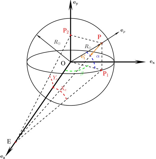
Sketch showing the geometry of the problem and the different reference frames employed in Section 1.3.2. The reference frame {ex, ey, ez} is centered at the Sun’s center ‘O’. The observed point at the Sun’s surface is denoted by ’P’. The observer is located at the point ‘E’, denoting the Earth. The vector OP is parallel to eρ, while EP is parallel to e *l .
5Note that the most general momentum equation would also include, in the right-hand term of Equation (17), the terms corresponding to the viscous forces: \(\mu _1 \nabla ^2 v\) and \([\mu _2 + (1/3)\mu _1 ]\nabla (\nabla v)\), where the coefficients μ1 and μ2 are often referred to as shear viscosity and bulk viscosity, respectively.
6According to Equation (12), z and τc have opposite signs. This indicates that τc decreases when z increases and, therefore, τc decreases from the photosphere to the corona.
7We shall mention here that, in order to provide the values of the derivatives in terms of the geometrical height instead of the optical depth, we have assumed that hydrostatic equilibrium holds (see Section 1.3.3).
8Thin in this context means that the thin flux-tube approximation (Spruit, 1981) can be applied. This reduces the problem to a 1D problem: it does so by assuming that the flux tube’s radius is much smaller than the pressure scale height.
9The elevation angle is defined as (1-ζ) (see Equation 10). Thus, small elevation angles correspond to horizontal magnetic fields (contained in the solar surface) and large elevation angles indicate magnetic fields that are rather vertical (perpendicular to the solar surface).
10SIR-like inversions refer to inversions of spectropolarimetric data where the physical parameters are allowed to vary with optical depth X(τc) (Equation 2). This is discussed in some detail in Section 1.3.

References
Abramenko, V.I., 1986, “The accuracy of potential field restoration using the Neumann problem”, Soln. Dannye, 1986, 83–89. [ADS] (Cited on page 12.)
Abramenko, V.I., Wang, T. and Yurchishin, V.B., 1996, “Analysis of Electric Current Helicity in Active Regions on the Basis of Vector Magnetograms”, Solar Phys., 168, 75–89. [DOI], [ADS] (Cited on page 40.)
Alissandrakis, C.E., 1981, “On the Computation of Constant α Force-free Magnetic Field”, Astron. Astrophys., 100, 197.200. [ADS] (Cited on page 12.)
Asensio Ramos, A., Trujillo Bueno, J. and Landi Degl’Innocenti, E., 2008, “Advanced Forward Modeling and Inversion of Stokes Profiles Resulting from the Joint Action of the Hanle and Zeeman Effects”, Astrophys. J., 683, 542.565. [DOI], [ADS], [arXiv:0804.2695 [astro-ph]] (Cited on page 7.)
Auer, L.H. and Heasley, J.N., 1978, “The origin of broad-band circular polarization in sunspots”, Astron. Astrophys., 64, 67–71. [ADS] (Cited on page 66.)
Auer, L.H., Heasley, J.N. and House, L.L., 1977, “Non-LTE line formation in the presence of magnetic fields”, Astrophys. J., 216, 531–539. [DOI], [ADS] (Cited on page 7.)
Balthasar, H. and Gömöry, P., 2008, “The three-dimensional structure of sunspots. I. The height dependence of the magnetic field”, Astron. Astrophys., 488, 1085–1092. [DOI], [ADS] (Cited on pages 29, 30, and 33.)
Balthasar, H., Schleicher, H., Bendlin, C. and Volkmer, R., 1996, “Two-dimensional spectroscopy of sunspots. I. Intensity, velocity, and velocity power maps of a sunspot”, Astron. Astrophys., 315, 603–609. [ADS] (Cited on pages 49 and 53.)
Beck, C., 2011, “An uncombed inversion of multiwavelength observations reproducing the net circular polarization in a sunspot’s penumbra”, Astron. Astrophys., 525, A133. [DOI], [ADS], [arXiv:1010.2095 [astro-ph.SR]] (Cited on page 31.)
Beckers, J.M., 1968, “High-resolution measurements of photosphere and sunspot velocity and magnetic fields using a narrow-band birefringent filter”, Solar Phys., 3, 258–268. [DOI], [ADS] (Cited on pages 51 and 53.)
Beckers, J.M., 1969a, “The Profiles of Fraunhofer Lines in the Presence of Zeeman Splitting. I: The Zeeman Triplet”, Solar Phys., 9, 372–386. [DOI], [ADS] (Cited on page 6.)
Beckers, J.M., 1969b, “The Profiles of Fraunhofer Lines in the Presence of Zeeman Splitting. II: Zeeman Multiplets for Dipole and Quadrupole Radiation”, Solar Phys., 10, 262–267. [DOI], [ADS] (Cited on page 6.)
Beckers, J.M. and Schröter, E.H., 1969a, “The Intensity, Velocity and Magnetic Structure of a Sunspot Region. IV: Properties of a Unipolar Sunspot”, Solar Phys., 10, 384–403. [DOI], [ADS] (Cited on page 47.)
Beckers, J.M. and Schröter, E.H., 1969b, “The Intensity, Velocity and Magnetic Structure of a Sunspot Region. IV: Properties of a Unipolar Sunspot”, Solar Phys., 10, 384–403. [DOI], [ADS] (Cited on page 45.)
Bello González, N., Okunev, O.V., Domínguez Cerdeña, I., Kneer, F. and Puschmann, K.G., 2005, “Polarimetry of sunspot penumbrae with high spatial resolution”, Astron. Astrophys., 434, 317–327. [DOI], [ADS] (Cited on page 23.)
Bellot Rubio, L.R., 2006, “Stokes Inversion Techniques: Recent Advances and New Challenges”, in Solar Polarization 4, Proceedings of the conference held in Boulder, Colorado, USA, 19 - 23 September, 2005, (Eds.) Casini, R., Lites, B.W., vol. 358 of ASP Conference Series, pp. 107–118, Astronomical Society of the Pacific, San Francisco. [ADS] (Cited on page 7.)
Bellot Rubio, L.R., Ruiz Cobo, B. and Collados, M., 1998, “An Hermitian Method for the Solution of Polarized Radiative Transfer Problems”, Astrophys. J., 506, 805–817. [DOI], [ADS] (Cited on page 7.)
Bellot Rubio, L.R., Collados, M., Ruiz Cobo, B. and Rodríguez Hidalgo, I., 2000, “Oscillations in the Photosphere of a Sunspot Umbra from the Inversion of Infrared Stokes Profiles”, Astrophys. J., 534, 989–996. [DOI], [ADS] (Cited on page 31.)
Bellot Rubio, L.R., Collados, M., Ruiz Cobo, B. and Rodríguez Hidalgo, I., 2002, “Photospheric structure of an extended penumbra”, Nuovo Cimento C, 25, 543–549. [ADS] (Cited on pages 23 and 31.)
Bellot Rubio, L.R., Balthasar, H. and Collados, M., 2004, “Two magnetic components in sunspot penumbrae”, Astron. Astrophys., 427, 319–334. [DOI], [ADS] (Cited on pages 13, 53, 58, and 60.)
Bellot Rubio, L.R., Langhans, K. and Schlichenmaier, R., 2005, “Multi-line spectroscopy of darkcored penumbral filaments”, Astron. Astrophys., 443, L7–L10. [DOI], [ADS] (Cited on pages 58 and 64.)
Bellot Rubio, L.R., Schlichenmaier, R. and Tritschler, A., 2006, “Two-dimensional spectroscopy of a sunspot. III. Thermal and kinematic structure of the penumbra at 0.5 arcsec resolution”, Astron. Astrophys., 453, 1117–1127. [DOI], [ADS], [astro-ph/0601423] (Cited on page 53.)
Bellot Rubio, L.R., Tsuneta, S., Ichimoto, K., Katsukawa, Y., Lites, B.W., Nagata, S., Shimizu, T., Shine, R.A., Suematsu, Y., Tarbell, T.D., Title, A.M. and del Toro Iniesta, J.C., 2007a, “Vector Spectropolarimetry of Dark-cored Penumbral Filaments with Hinode”, Astrophys. J. Lett., 668, L91–L94. [DOI], [ADS], [arXiv:0708.2791] (Cited on page 64.)
Bellot Rubio, L.R., Tsuneta, S., Ichimoto, K., Katsukawa, Y., Lites, B.W., Nagata, S., Shimizu, T., Shine, R.A., Suematsu, Y., Tarbell, T.D., Title, A.M. and del Toro Iniesta, J.C., 2007b, “Vector Spectropolarimetry of Dark-cored Penumbral Filaments with Hinode”, Astrophys. J. Lett., 668, L91–L94. [DOI], [ADS], [arXiv:0708.2791] (Cited on page 23.)
Bellot Rubio, L.R., Schlichenmaier, R. and Langhans, K., 2010, “Searching for Overturning Convection in Penumbral Filaments: Slit Spectroscopy at 0.2 arcsec Resolution”, Astrophys. J., 725, 11–16. [DOI], [ADS], [arXiv:1009.5650 [astro-ph.SR]] (Cited on pages 60 and 71.)
Berger, T.E. and Berdyugina, S.V., 2003, “The Observation of Sunspot Light-Bridge Structure and Dynamics”, Astrophys. J. Lett., 589, L117–L121. [DOI], [ADS] (Cited on page 45.)
Bharti, L., Jain, R. and Jaaffrey, S.N.A., 2007, “Evidence for Magnetoconvection in Sunspot Umbral Dots”, Astrophys. J. Lett., 665, L79–L82. [DOI], [ADS] (Cited on page 45.)
Bharti, L., Joshi, C., Jaaffrey, S.N.A. and Jain, R., 2009, “Spectropolarimetery of umbral fine structures from Hinode: evidence for magnetoconvection”, Mon. Not. R. Astron. Soc., 393, 65–70. [DOI], [ADS], [arXiv:0811.1722] (Cited on page 43.)
Bharti, L., Solanki, S.K. and Hirzberger, J., 2010, “Evidence for Convection in Sunspot Penumbrae”, Astrophys. J. Lett., 722, L194–L198. [DOI], [ADS], [arXiv:1009.2919 [astro-ph.SR]] (Cited on pages 60 and 65.)
Borrero, J.M., 2007, “The structure of sunspot penumbrae. IV. MHS equilibrium for penumbral flux tubes and the origin of dark core penumbral filaments and penumbral grains”, Astron. Astrophys., 471, 967–975. [DOI], [ADS], [arXiv:0704.3219] (Cited on page 64.)
Borrero, J.M., 2009, “Models and observations of sunspot penumbrae”, Sci. China Ser. G, 52, 1670–1677. [DOI], [ADS], [arXiv:0810.0080] (Cited on pages 60 and 70.)
Borrero, J.M. and Solanki, S.K., 2008, “Are There Field-Free Gaps near τ = 1 in Sunspot Penumbrae?”, Astrophys. J., 687, 668–677. [DOI], [ADS], [arXiv:0806.4454] (Cited on pages 31, 52, 68, and 70.)
Borrero, J.M. and Solanki, S.K., 2010, “Convective Motions and Net Circular Polarization in Sunspot Penumbrae”, Astrophys. J., 709, 349–357. [DOI], [ADS], [arXiv:0911.2570 [astro-ph.SR]] (Cited on pages 68 and 70.)
Borrero, J.M., Solanki, S.K., Bellot Rubio, L.R., Lagg, A. and Mathew, S.K., 2004, “On the fine structure of sunspot penumbrae. I. A quantitative comparison of two semiempirical models with implications for the Evershed effect”, Astron. Astrophys., 422, 1093–1104. [DOI], [ADS] (Cited on pages 31 and 53.)
Borrero, J.M., Lagg, A., Solanki, S.K. and Collados, M., 2005, “On the fine structure of sunspot penumbrae. II. The nature of the Evershed flow”, Astron. Astrophys., 436, 333–345. [DOI], [ADS], [arXiv:astro-ph/0503677] (Cited on page 53.)
Borrero, J.M., Solanki, S.K., Lagg, A., Socas-Navarro, H. and Lites, B.W., 2006, “On the fine structure of sunspot penumbrae. III. The vertical extension of penumbral filaments”, Astron. Astrophys., 450, 383–393. [DOI], [ADS], [astro-ph/0510586] (Cited on pages 67 and 69.)
Borrero, J.M., Bellot Rubio, L.R. and Müller, D.A.N., 2007, “Flux Tubes as the Origin of Net Circular Polarization in Sunspot Penumbrae”, Astrophys. J. Lett., 666, L133–L136. [DOI], [ADS], [arXiv:0707.4145] (Cited on pages 68 and 69.)
Borrero, J.M., Lites, B.W. and Solanki, S.K., 2008, “Evidence of magnetic field wrapping around penumbral filaments”, Astron. Astrophys., 481, L13–L16. [DOI], [ADS], [arXiv:0712.2548] (Cited on pages 54 and 56.)
Borrero, J.M., Tomczyk, S., Kubo, M., Socas-Navarro, H., Schou, J., Couvidat, S. and Bogart, R.S., 2010, “VFISV: Very Fast Inversion of the Stokes Vector for the Helioseismic and Magnetic Imager”, Solar Phys., in press, 35. [DOI], [ADS], [arXiv:0901.2702 [astro-ph.IM]] (Cited on page 9.)
Brants, J.J. and Zwaan, C., 1982, “The structure of sunspots. IV. Magnetic field strengths in small sunspots and pores”, Solar Phys., 80, 251–258. [DOI], [ADS] (Cited on page 24.)
Bray, R.J. and Loughhead, R.E., 1979, Sunspots, Dover, New York. [ADS] (Cited on page 50.)
Brosius, J.W. and White, S.M., 2006, “Radio Measurements of the Height of Strong Coronal Magnetic Fields Above Sunspots at the Solar Limb”, Astrophys. J. Lett., 641, L69–L72. [DOI], [ADS] (Cited on page 7.)
Brosius, J.W., Landi, E., Cook, J.W., Newmark, J.S., Gopalswamy, N. and Lara, A., 2002, “Measurements of Three-dimensional Coronal Magnetic Fields from Coordinated Extreme-Ultraviolet and Radio Observations of a Solar Active Region Sunspot”, Astrophys. J., 574, 453–466. [DOI], [ADS] (Cited on page 7.)
Brummell, N.H., Tobias, S.M., Thomas, J.H. and Weiss, N.O., 2008, “Flux Pumping and Magnetic Fields in the Outer Penumbra of a Sunspot”, Astrophys. J., 686, 1454–1465. [DOI], [ADS] (Cited on page 71.)
Cabrera Solana, D., 2007, Temporal evolution of the Evershed flow and its magnetic properties, Ph.D. Thesis, Universidad de Granada, Granada, Spain. [ADS] (Cited on page 31.)
Cabrera Solana, D., Bellot Rubio, L.R., Beck, C. and del Toro Iniesta, J.C., 2006, “Inversion of Visible and IR Stokes Profiles in Sunspots”, in Solar Polarization 4, Proceedings of the conference held in Boulder, Colorado, USA, 19 - 23 September, 2005, (Eds.) Casini, R., Lites, B.W., vol. 358 of ASP Conference Series, pp. 25–30, Astronomical Society of the Pacific, San Francisco. [ADS] (Cited on page 31.)
Cabrera Solana, D., Bellot Rubio, L.R., Borrero, J.M. and del Toro Iniesta, J.C., 2008, “Temporal evolution of the Evershed flow in sunspots. II. Physical properties and nature of Evershed clouds”, Astron. Astrophys., 477, 273–283. [DOI], [ADS], [arXiv:0709.1601] (Cited on page 31.)
Cameron, R.H., Gizon, L., Schunker, H. and Pietarila, A., 2011, “Constructing Semi-Empirical Sunspot Models for Helioseismology”, Solar Phys., 268, 293–308. [DOI], [ADS], [arXiv:1003.0528 [astro-ph.SR]] (Cited on page 22.)
Canfield, R.C., de La Beaujardiere, J.-F., Fan, Y., Leka, K.D., McClymont, A.N., Metcalf, T.R., Mickey, D.L., Wuelser, J.-P. and Lites, B.W., 1993, “The morphology of flare phenomena, magnetic fields, and electric currents in active regions. I. Introduction and methods”, Astrophys. J., 411, 362–369. [DOI], [ADS] (Cited on page 12.)
Carroll, T.A. and Kopf, M., 2008, “Zeeman-tomography of the solar photosphere. Three-dimensional surface structures retrieved from Hinode observations”, Astron. Astrophys., 481, L37–L40. [DOI], [ADS], [arXiv:0803.1048] (Cited on page 20.)
Carroll, T.A. and Staude, J., 2001, “The inversion of Stokes profiles with artificial neural networks”, Astron. Astrophys., 378, 316–326. [DOI], [ADS] (Cited on pages 7 and 20.)
Casini, R., Manso Sainz, R. and Low, B.C., 2009, “Polarimetric Diagnostics of Unresolved Chromospheric Magnetic Fields”, Astrophys. J. Lett., 701, L43–L46. [DOI], [ADS], [arXiv:0811.0512] (Cited on page 7.)
Charbonneau, P., 1995, “Genetic Algorithms in Astronomy and Astrophysics”, Astrophys. J. Suppl. Ser., 101, 309–334. [DOI], [ADS] (Cited on page 7.)
Cheung, M.C.M., Rempel, M., Title, A.M. and Schüssler, M., 2010, “Simulation of the Formation of a Solar Active Region”, Astrophys. J., 720, 233–244. [DOI], [ADS], [arXiv:1006.4117 [astro-ph.SR]] (Cited on page 47.)
Choudhuri, A.R., 1986, “The dynamics of magnetically trapped fluids. I. Implications for umbral dots and penumbral grains”, Astrophys. J., 302, 809–825. [DOI], [ADS] (Cited on page 50.)
Choudhuri, A.R., Chatterjee, P. and Nandy, D., 2004, “Helicity of Solar Active Regions from a Dynamo Model”, Astrophys. J. Lett., 615, L57–L60. [DOI], [ADS] (Cited on page 40.)
Collados, M., Martínez Pillet, V., Ruiz Cobo, B., del Toro Iniesta, J.C. and Vázquez, M., 1994, “Observed differences between large and small sunspots”, Astron. Astrophys., 291, 622–634. [ADS] (Cited on page 24.)
Cowling, T.G., 1953, “Solar Electrodynamics”, in The Solar System, Vol. 1: The Sun, (Ed.) Kuiper, G.P., p. 532, University of Chicago Press, Chicago. [ADS] (Cited on page 43.)
Cram, L.E. and Thomas, J.H. (Eds.), 1981, The Physics of Sunspots, Proceedings of the Conference, Sunspot, NM, July 14 - 17, 1981, Sacramento Peak Observatory, Sunspot, NM. [ADS] (Cited on page 51.)
Crouch, A.D. and Barnes, G., 2008, “Resolving the Azimuthal Ambiguity in Vector Magnetogram Data with the Divergence-Free Condition: Theoretical Examination”, Solar Phys., 247, 25–37. [DOI], [ADS] (Cited on page 12.)
Cuperman, S., Ofman, L. and Semel, M., 1990, “Determination of force-free magnetic fields above the photosphere using three-component boundary conditions: moderately non-linear case”, Astron. Astrophys., 230, 193–199. [ADS] (Cited on page 12.)
Cuperman, S., Li, J. and Semel, M., 1992, “Magnetic shear-based removal of the 180° ambiguity in the observed transverse photospheric magnetic field: feasibility and limitations”, Astron. Astrophys., 265, 296–307. [ADS] (Cited on page 12.)
Danielson, R.E., 1961a, “The Structure of Sunspot Penumbras. I. Observations”, Astrophys. J., 134, 275–288. [DOI], [ADS] (Cited on page 47.)
Danielson, R.E., 1961b, “The Structure of Sunspot Penumbras. II. Theoretical”, Astrophys. J., 134, 289–311. [DOI], [ADS] (Cited on page 51.)
Degenhardt, D., 1991, “Stationary siphon flows in thin magnetic flux tubes. II. Radiative heat exchange with the surroundings”, Astron. Astrophys., 248, 637–646. [ADS] (Cited on page 52.)
Degenhardt, D. and Wiehr, E., 1991, “Spatial variation of the magnetic field inclination in a sunspot penumbra”, Astron. Astrophys., 252, 821–826. [ADS] (Cited on page 48.)
del Toro Iniesta, J.C., 2003a, “Interpretation of observations by inversion”, Astron. Nachr., 324, 383–387. [DOI], [ADS] (Cited on page 7.)
del Toro Iniesta, J.C., 2003b, Introduction to Spectropolarimetry, Cambridge University Press, Cambridge; New York. [ADS], [Google Books] (Cited on page 9.)
del Toro Iniesta, J.C., Bellot Rubio, L.R. and Collados, M., 2001, “Cold, Supersonic Evershed Downflows in a Sunspot”, Astrophys. J. Lett., 549, L139–L142. [DOI], [ADS] (Cited on pages 58 and 60.)
DeRosa, M.L., Schrijver, C.J., Barnes, G., Leka, K.D., Lites, B.W., Aschwanden, M.J., Amari, T., Canou, A., McTiernan, J.M., Régnier, S., Thalmann, J.K., Valori, G., Wheatland, M.S., Wiegelmann, T., Cheung, M.C.M., Conlon, P.A., Fuhrmann, M., Inhester, B. and Tadesse, T., 2009, “A Critical Assessment of Nonlinear Force-Free Field Modeling of the Solar Corona for Active Region 10953”, Astrophys. J., 696, 1780–1791. [DOI], [ADS], [arXiv:0902.1007 [astro-ph.SR]] (Cited on page 22.)
Elmore, D.F., Lites, B.W., Tomczyk, S., Skumanich, A.P., Dunn, R.B., Schuenke, J.A., Streander, K.V., Leach, T.W., Chambellan, C.W. and Hull, H.K., 1992, “The Advanced Stokes Polarimeter: A new instrument for solar magnetic field research”, in Polarization analysis and measurement, Proceedings of the Meeting, San Diego, CA, July 19 - 21, 1992, (Eds.) Goldstein, D.H., Chipman, R.A., vol. 1746 of Proc. SPIE, pp. 22–33, SPIE, Bellingham, WA. [ADS] (Cited on page 12.)
Evershed, J., 1909, “Radial movement in sun-spots”, Mon. Not. R. Astron. Soc., 69, 454–457. [ADS] (Cited on pages 42 and 50.)
Fan, Y. and Gong, D., 2000, “On the twist of emerging flux loops in the solar convection zone”, Solar Phys., 192, 141–157. [DOI], [ADS] (Cited on page 40.)
Franz, M. and Schlichenmaier, R., 2009, “The velocity field of sunspot penumbrae. I. A global view”, Astron. Astrophys., 508, 1453–1460. [DOI], [ADS], [arXiv:0909.4744 [astro-ph.SR]] (Cited on pages 58, 60, and 71.)
Frutiger, C., Solanki, S.K., Fligge, M. and Bruls, J.H.M.J., 1999, “Inversion of Stokes profiles”, in Solar Polarization, Proceedings of an international workshop held in Bangalore, India, 12 - 16 October, 1998, (Eds.) Nagendra, K.N., Stenflo, J.O., vol. 243 of Astrophysics and Space Science Library, pp. 281–290, Kluwer, Boston. [ADS] (Cited on pages 9, 19, and 27.)
Galloway, D.J., 1975, “Fine structure and Evershed motions in the sunspot penumbra”, Solar Phys., 44, 409–415. [DOI], [ADS] (Cited on page 51.)
Gary, G.A., 1989, “Linear force-free magnetic fields for solar extrapolation and interpretation”, Astrophys. J. Suppl. Ser., 69, 323–348. [DOI], [ADS] (Cited on page 12.)
Gary, G.A. and Demoulin, P., 1995, “Reduction, analysis, and properties of electric current systems in solar active regions”, Astrophys. J., 445, 982–998. [DOI], [ADS] (Cited on page 12.)
Georgoulis, M.K., 2005, “A New Technique for a Routine Azimuth Disambiguation of Solar Vector Magnetograms”, Astrophys. J. Lett., 629, L69–L72. [DOI], [ADS] (Cited on page 12.)
Georgoulis, M.K. and LaBonte, B.J., 2004, “Vertical Lorentz Force and Cross-Field Currents in the Photospheric Magnetic Fields of Solar Active Regions”, Astrophys. J., 615, 1029–1041. [DOI], [ADS] (Cited on page 34.)
Gizon, L. and Birch, A.C., 2005, “Local Helioseismology”, Living Rev. Solar Phys., 2, lrsp-2005-6. [ADS]. URL (accessed 30 May 2011): http://www.livingreviews.org/lrsp-2005-6 (Cited on page 47.
Gokhale, M.H. and Zwaan, C., 1972, “The Structure of Sunspots. I: Observational Constraints: Current Sheet Models”, Solar Phys., 26, 52–75. [DOI], [ADS] (Cited on page 47.)
Grossmann-Doerth, U., Schmidt, W. and Schroeter, E.H., 1986, “Size and temperature of umbral dots”, Astron. Astrophys., 156, 347–353. [ADS] (Cited on page 43.)
Grossmann-Doerth, U., Larsson, B. and Solanki, S.K., 1988, “Contribution and response functions for Stokes line profiles formed in a magnetic field”, Astron. Astrophys., 204, 266–274. [ADS] (Cited on page 8.)
Hagyard, M.J., 1987, “Changes in measured vector magnetic fields when transformed into heliographic coordinates”, Solar Phys., 107, 239–246. [DOI], [ADS] (Cited on page 13.)
Hagyard, M.J., Teuber, D., West, E.A., Tandberg-Hanssen, E., Henze Jr, W., Beckers, J.M., Bruner, M., Hyder, C.L. and Woodgate, B.E., 1983, “Vertical gradients of sunspot magnetic fields”, Solar Phys., 84, 13–31. [DOI], [ADS] (Cited on page 27.)
Hale, G.E., 1908, “On the Probable Existence of a Magnetic Field in Sun-Spots”, Astrophys. J., 28, 315–343. [DOI], [ADS] (Cited on page 6.)
Hale, G.E., 1925, “Nature of the Hydrogen Vortices Surrounding Sun-spots”, Publ. Astron. Soc. Pac., 37, 268–270. [DOI], [ADS] (Cited on page 40.)
Hale, G.E., 1927, “The Fields of Force in the Atmosphere of the Sun”, Nature, 119, 708–714. [DOI], [ADS] (Cited on page 40.)
Heinemann, T., Nordlund, Å., Scharmer, G.B. and Spruit,.C., 2007, “MHD Simulations of Penumbra Fine Structure”, Astrophys. J., 669, 1390.1394. [DOI], [ADS], [astro-ph/0612648] (Cited on page 70.)
Henson, G.D. and Kemp, J.C., 1984, “Broad-band circular polarimetry of sunspots, 0.4-1.7 microns: Spatial scans with a 3.4 arc sec diameter aperture”, Solar Phys., 93, 289–299. [DOI], [ADS] (Cited on page 66.)
Hirzberger, J. and Kneer, F., 2001, “2D-spectroscopy of the Evershed flow in sunspots”, Astron. Astrophys., 378, 1078–1086. [DOI], [ADS] (Cited on page 53.)
Hirzberger, J., Bonet, J.A., Sobotka, M., Vázquez, M. and Hanslmeier, A., 2002, “Fine structure and dynamics in a light bridge inside a solar pore”, Astron. Astrophys., 383, 275–282. [DOI], [ADS] (Cited on page 45.)
Ichimoto, K., 1987, “Evershed effect observed in various solar photospheric lines. I. Dependence of the velocity distribution across the penumbra on the equivalent width”, Publ. Astron. Soc. Japan, 39, 329–342. [ADS] (Cited on page 68.)
Ichimoto, K., 1988, “Evershed effect observed in various solar photospheric lines. II. Dependence on the excitation potential”, Publ. Astron. Soc. Japan, 40, 103–119. [ADS] (Cited on page 51.)
Ichimoto, K., 2010, “The Evershed Effect with SOT/Hinode”, in Magnetic Coupling between the Interior and Atmosphere of the Sun, Proceedings of ‘Centenary Commemoration of the Discovery of the Evershed Effect’, Indian Institute of Astrophysics, Bangalore, India, December 2 - 5, 2008, (Eds.) Hasan, S.S., Rutten, R.J., Astrophysics and Space Science Proceedings, pp. 186–192, Springer, Berlin; Heidelberg. [DOI], [ADS], [arXiv:0903.2605 [astro-ph.SR]] (Cited on pages 60 and 70.)
Ichimoto, K., Shine, R.A., Lites, B.W., Kubo, M., Shimizu, T., Suematsu, Y., Tsuneta, S., Katsukawa, Y., Tarbell, T.D., Title, A.M., Nagata, S., Yokoyama, T. and Shimojo, M., 2007a, “Fine-Scale Structures of the Evershed Effect Observed by the Solar Optical Telescope aboard Hinode”, Publ. Astron. Soc. Japan, 59, S593–S599. [ADS] (Cited on pages 53, 58, and 63.)
Ichimoto, K., Suematsu, Y., Tsuneta, S., Katsukawa, Y., Shimizu, T., Shine, R.A., Tarbell, T.D., Title, A.M., Lites, B.W., Kubo, M. and Nagata, S., 2007b, “Twisting Motions of Sunspot Penumbral Filaments”, Science, 318, 1597–1599. [DOI], [ADS] (Cited on pages 60 and 65.)
Ichimoto, K., Lites, B.W., Elmore, D., Suematsu, Y., Tsuneta, S., Katsukawa, Y., Shimizu, T., Shine, R.A., Tarbell, T., Title, A.M., Kiyohara, J., Shinoda, K., Card, G., Lecinski, A., Streander, K., Nakagiri, M., Miyashita, M., Noguchi, M., Hoffmann, C. and Cruz, T., 2008a, “Polarization Calibration of the Solar Optical Telescope onboard Hinode”, Solar Phys., 249, 233–261. [DOI], [ADS] (Cited on page 9.)
Ichimoto, K., Tsuneta, S., Suematsu, Y., Katsukawa, Y., Shimizu, T., Lites, B.W., Kubo, M., Tarbell, T.D., Shine, R.A., Title, A.M. and Nagata, S., 2008b, “Net circular polarization of sunspots in high spatial resolution”, Astron. Astrophys., 481, L9–L12. [DOI], [ADS] (Cited on page 68.)
Illing, R.M.E., Landman, D.A. and Mickey, D.L., 1974a, “Observations of Broad-band Circular Polarization in Sunspots: Magnetic Field Correspondence”, Astron. Astrophys., 37, 97–99. [ADS] (Cited on page 66.)
Illing, R.M.E., Landman, D.A. and Mickey, D.L., 1974b, “Broad-band circular and linear polarization in sunspots Center-to-limb variation”, Astron. Astrophys., 35, 327–331. [ADS] (Cited on page 66.)
Illing, R.M.E., Landman, D.A. and Mickey, D.L., 1975, “Broad-band Circular Polarization of Sunspots: Spectral Dependence and Theory”, Astron. Astrophys., 41, 183–185. [ADS] (Cited on page 67.)
Jahn, K. and Schmidt, H.U., 1994a, “Thick penumbra in a magnetostatic sunspot model”, Astron. Astrophys., 290, 295–317. [ADS], [astro-ph/9410011] (Cited on page 53.)
Jahn, K. and Schmidt, H.U., 1994b, “Thick penumbra in a magnetostatic sunspot model”, Astron. Astrophys., 290, 295–317. [ADS], [astro-ph/9410011] (Cited on page 22.)
Ji, H.-S., Song, M.-T., Zhang, Y.-A. and Song, S.-M., 2003, “The horizontal and vertical electric currents in three solar active regions and their relations with flares”, Chin. Astron. Astrophys., 27, 79–88. [DOI], [ADS] (Cited on page 34.)
Jin, C.L., Qu, Z.Q., Xu, C.L., Zhang, X.Y. and Sun, M.G., 2006, “The Relationships of Sunspot Magnetic Field Strength with Sunspot Area, Umbral Area and Penumbra-Umbra Radius Ratio”, Astrophys. Space Sci., 306, 23–27. [DOI], [ADS] (Cited on page 24.)
Johannesson, A., 1993, “The fine scale dynamics of a sunspot penumbra”, Astron. Astrophys., 273, 633–641. [ADS] (Cited on page 58.)
Jurčák, J. and Bellot Rubio, L.R., 2008, “Penumbral models in the light of Hinode spectropolarimetric observations”, Astron. Astrophys., 481, L17–L20. [DOI], [ADS], [arXiv:0711.1692] (Cited on page 54.)
Jurčák, J., Martínez Pillet, V. and Sobotka, M., 2006, “The magnetic canopy above light bridges”, Astron. Astrophys., 453, 1079–1088. [DOI], [ADS] (Cited on page 45.)
Jurčák, J., Bellot Rubio, L.R., Ichimoto, K., Katsukawa, Y., Lites, B.W., Nagata, S., Shimizu, T., Suematsu, Y., Tarbell, T.D., Title, A.M. and Tsuneta, S., 2007, “The Analysis of Penumbral Fine Structure Using an Advanced Inversion Technique”, Publ. Astron. Soc. Japan, 59, S601–S606. [ADS], [arXiv:0707.1560] (Cited on pages 54 and 55.)
Katsukawa, Y., Berger, T.E., Ichimoto, K., Lites, B.W., Nagata, S., Shimizu, T., Shine, R.A., Suematsu, Y., Tarbell, T.D., Title, A.M. and Tsuneta, S., 2007, “Small-Scale Jetlike Features in Penumbral Chromospheres”, Science, 318, 1594–1597. [DOI], [ADS] (Cited on page 49.)
Khomenko, E. and Collados, M., 2008, “Magnetohydrostatic Sunspot Models from Deep Subphotospheric to Chromospheric Layers”, Astrophys. J., 689, 1379–1387. [DOI], [ADS], [arXiv:0808.3571] (Cited on page 22.)
Kitiashvili, I.N., Kosovichev, A.G., Wray, A.A. and Mansour, N.N., 2009, “Traveling Waves of Magnetoconvection and the Origin of the Evershed Effect in Sunspots”, Astrophys. J. Lett., 700, L178–L181. [DOI], [ADS], [arXiv:0904.3599 [astro-ph.SR]] (Cited on page 70.)
Kneer, F., 1972, “Profile magnetisch aufspaltender Linien in Sonnenflecken [Profiles of Magnetically Split Lines in Sunspots]”, Astron. Astrophys., 18, 47–50. [ADS] (Cited on page 27.)
Kopp, G. and Rabin, D., 1992, “A relation between magnetic field strength and temperature in sunspots”, Solar Phys., 141, 253–265. [DOI], [ADS] (Cited on page 24.)
Kotov, V.A., 1970, “Magnetic field and electric currents of a unipolar sunspot”, Izv. Krymsk. Astrof. Obs., 41, 67–88. [ADS] (Cited on pages 27 and 29.)
Kozlova, L. and Somov, B., 2009, “Determination of the gradient magnetic field above a sunspot based on observations of the HeI and FeI infrared lines”, Moscow Univ. Phys. Bull., 64(5), 541–545. [DOI] (Cited on page 27.)
Lagg, A., Woch, J., Krupp, N. and Solanki, S.K., 2004, “Retrieval of the full magnetic vector with the He I multiplet at 1083 nm. Maps of an emerging flux region”, Astron. Astrophys., 414, 1109–1120. [DOI], [ADS] (Cited on page 7.)
Landi Degl’Innocenti, E. and Landi Degl’Innocenti, M., 1972, “Quantum Theory of Line Formation in a Magnetic Field”, Solar Phys., 27, 319–329. [DOI], [ADS] (Cited on page 7.)
Landi Degl’Innocenti, E. and Landi Degl’Innocenti, M., 1977, “Response functions for magnetic lines”, Astron. Astrophys., 56, 111–115. [ADS] (Cited on page 8.)
Landi Degl’Innocenti, E. and Landolfi, M. (Eds.), 2004, Polarization in Spectral Lines, vol. 307 of Astrophysics and Space Science Library, Kluwer, Dordrecht; Boston. [ADS] (Cited on page 7.)
Landolfi, M. and Landi Degl’Innocenti, E., 1996, “Net Circular Polarization in Magnetic Spectral Lines Produced by Velocity Gradients: Some Analytical Results”, Solar Phys., 164, 191–202. [DOI], [ADS] (Cited on page 66.)
Langhans, K., Scharmer, G.B., Kiselman, D., Löfdahl, M.G. and Berger, T.E., 2005, “Inclination of magnetic fields and flows in sunspot penumbrae”, Astron. Astrophys., 436, 1087–1101. [DOI], [ADS] (Cited on page 48.)
Langhans, K., Scharmer, G.B., Kiselman, D. and Löfdahl, M.G., 2007, “Observations of dark-cored filaments in sunspot penumbrae”, Astron. Astrophys., 464, 763–774. [DOI], [ADS] (Cited on page 64.)
Leka, K.D., 1997, “The Vector Magnetic Fields and Thermodynamics of Sunspot Light Bridges: The Case for Field-free Disruptions in Sunspots”, Astrophys. J., 484, 900–919. [DOI], [ADS] (Cited on page 45.)
Leka, K.D. and Metcalf, T.R., 2003, “Active-Region Magnetic Structure Observed in the Photosphere and Chromosphere”, Solar Phys., 212, 361–378. [DOI], [ADS] (Cited on pages 27 and 29.)
Leka, K.D., Barnes, G., Crouch, A.D., Metcalf, T.R., Gary, G.A., Jing, J. and Liu, Y., 2009, “Resolving the 180° Ambiguity in Solar Vector Magnetic Field Data: Evaluating the Effects of Noise, Spatial Resolution, and Method Assumptions”, Solar Phys., 260, 83–108. [DOI], [ADS] (Cited on page 12.)
Li, J., van Ballegooijen, A.A. and Mickey, D., 2009, “Vector Magnetic Fields and Electric Currents From the Imaging Vector Magnetograph”, Astrophys. J., 692, 1543–1560. [DOI], [ADS], [arXiv:0811.0054] (Cited on page 33.)
Lites, B.W., Bida, T.A. and Scharmer, G.B., 1989, “The Magnetic Field Strength of Umbral Dots”, Bull. Am. Astron. Soc., 21, 854. [ADS] (Cited on page 43.)
Lites, B.W., Skumanich, A.P. and Scharmer, G.B., 1990, “High-resolution spectra of solar magnetic features. I. Analysis of penumbral fine structure”, Astrophys. J., 355, 329–341. [DOI], [ADS] (Cited on pages 48 and 53.)
Lites, B.W., Elmore, D.F., Seagraves, P. and Skumanich, A.P., 1993, “Stokes Profile Analysis and Vector Magnetic Fields. VI. Fine Scale Structure of a Sunspot”, Astrophys. J., 418, 928–942. [DOI], [ADS] (Cited on pages 23 and 48.)
Lites, B.W., Scharmer, G.B., Berger, T.E. and Title, A.M., 2004, “Three-Dimensional Structure of the Active Region Photosphere as Revealed by High Angular Resolution”, Solar Phys., 221, 65–84. [DOI], [ADS] (Cited on page 44.)
Livingston, W., 2002, “Sunspots Observed to Physically Weaken in 2000-2001”, Solar Phys., 207, 41–45. [DOI], [ADS] (Cited on page 24.)
López Ariste, A. and Semel, M., 1999a, “DIAGONAL: A numerical solution of the Stokes transfer equation”, Astron. Astrophys. Suppl., 139, 417–424. [DOI], [ADS] (Cited on page 7.)
López Ariste, A. and Semel, M., 1999b, “Analytical solution of the radiative transfer equation for polarized light”, Astron. Astrophys., 350, 1089–1099. [ADS], [astro-ph/9909232] (Cited on pages 7 and 9.)
Loughhead, R.E., Bray, R.J. and Tappere, E.J., 1979, “Improved observations of sunspot umbral dots”, Astron. Astrophys., 79, 128–131. [ADS] (Cited on page 43.)
Low, B.C., 1975, “Nonisothermal magnetostatic equilibria in a uniform gravity field. I. Mathematical formulation”, Astrophys. J., 197, 251–255. [DOI], [ADS] (Cited on page 22.)
Low, B.C., 1980, “Exact static equilibrium of vertically oriented magnetic flux tubes. I. The Schlüter-Temesváry sunspot”, Solar Phys., 67, 57–77. [DOI], [ADS] (Cited on page 22.)
Makita, M., 1986, “An interpretation of the broad-band circular polarization of sunspots”, Solar Phys., 106, 269–286. [DOI], [ADS] (Cited on page 67.)
Makita, M. and Nemoto, K., 1976, “Magnetic field gradient in the sunspot umbra”, Publ. Astron. Soc. Japan, 28, 495–508. [ADS] (Cited on pages 27 and 29.)
Makita, M. and Ohki, Y., 1986, “The broad-band polarization of sunspots observed from 8 February 1981 to 30 August 1982”, Ann. Tokyo Obs., 21, 1–30. [ADS] (Cited on page 66.)
Maltby, P., 1977, “On the difference in darkness between sunspots”, Solar Phys., 55, 335–346. [DOI], [ADS] (Cited on page 20.)
Manso Sainz, R. and Trujillo Bueno, J., 2003, “Zero-Field Dichroism in the Solar Chromosphere”, Phys. Rev. Lett., 91, 111102. [DOI], [ADS], [astro-ph/0311455] (Cited on page 7.)
Márquez, I., Sánchez Almeida, J. and Bonet, J.A., 2006, “High-Resolution Proper Motions in a Sunspot Penumbra”, Astrophys. J., 638, 553–563. [DOI], [ADS], [arXiv:astro-ph/0510220] (Cited on page 60.)
Martínez Pillet, V., 2000, “Spectral signature of uncombed penumbral magnetic fields”, Astron. Astrophys., 361, 734–742. [ADS] (Cited on pages 66 and 67.)
Martínez Pillet, V. and Vazquez, M., 1993, “The continuum intensity-magnetic field relation in sunspot umbrae”, Astron. Astrophys., 270, 494–508. [ADS] (Cited on page 20.)
Martínez Pillet, V., Katsukawa, Y., Puschmann, K.G. and Ruiz Cobo, B., 2009, “Supersonic Continuation of the Evershed Flow Outside a Sunspot as Observed with Hinode”, Astrophys. J. Lett., 701, L79–L82. [DOI], [ADS] (Cited on page 64.)
Mathew, S.K., Lagg, A., Solanki, S.K., Collados, M., Borrero, J.M., Berdyugina, S., Krupp, N., Woch, J. and Frutiger, C., 2003, “Three dimensional structure of a regular sunspot from the inversion of IR Stokes profiles”, Astron. Astrophys., 410, 695–710. [DOI], [ADS] (Cited on pages 29, 30, 31, 38, and 52.)
Mathew, S.K., Solanki, S.K., Lagg, A., Collados, M., Borrero, J.M. and Berdyugina, S., 2004, “Thermal-magnetic relation in a sunspot and a map of its Wilson depression”, Astron. Astrophys., 422, 693–701. [DOI], [ADS] (Cited on pages 20, 36, 38, and 39.)
Metcalf, T.R., 1994, “Resolving the 180-degree ambiguity in vector magnetic field measurements: The ‘minimum’ energy solution”, Solar Phys., 155, 235–242. [DOI], [ADS] (Cited on page 12.)
Metcalf, T.R., Leka, K.D., Barnes, G., Lites, B.W., Georgoulis, M.K., Pevtsov, A.A., Balasubramaniam, K.S., Gary, G.A., Jing, J., Li, J., Liu, Y., Wang, H.N., Abramenko, V., Yurchyshyn, V. and Moon, Y.-J., 2006, “An Overview of Existing Algorithms for Resolving the 180° Ambiguity in Vector Magnetic Fields: Quantitative Tests with Synthetic Data”, Solar Phys., 237, 267–296. [DOI], [ADS] (Cited on pages 12, 13, and 33.)
Metcalf, T.R., De Rosa, M.L., Schrijver, C.J., Barnes, G., van Ballegooijen, A.A., Wiegelmann, T., Wheatland, M.S., Valori, G. and McTtiernan, J.M., 2008, “Nonlinear Force-Free Modeling of Coronal Magnetic Fields. II. Modeling a Filament Arcade and Simulated Chromospheric and Photospheric Vector Fields”, Solar Phys., 247, 269–299. [DOI], [ADS] (Cited on page 22.)
Meyer, F. and Schmidt, H.U., 1968, “A Model for the Evershed Flow in Sunspots”, Mitt. Astron. Gesellsch., 25, 194–197. [ADS] (Cited on page 52.)
Meyer, F., Schmidt, H.U., Wilson, P.R. and Weiss, N.O., 1974, “The growth and decay of sunspots”, Mon. Not. R. Astron. Soc., 169, 35–57. [ADS] (Cited on page 47.)
Meyer, F., Schmidt, H.U. and Weiss, N.O., 1977, “The stability of sunspots”, Mon. Not. R. Astron. Soc., 179, 741–761. [ADS] (Cited on pages 33 and 47.)
Mihalas, D., 1978, Stellar atmospheres, W.H. Freeman, San Francisco, 2nd edn. [ADS] (Cited on pages 7 and 19.)
Molowny-Horas, R., 1994, “Proper motion measurements of umbral and penumbral structure”, Solar Phys., 154, 29–39. [DOI], [ADS] (Cited on page 43.)
Montesinos, B. and Thomas, J.H., 1993, “Siphon flows in isolated magnetic flux tubes. V. Radiative flows with variable ionization”, Astrophys. J., 402, 314–325. [DOI], [ADS] (Cited on page 52.)
Moore, R.L., 1981, “Structure of the sunspot penumbra”, Astrophys. J., 249, 390–393. [DOI], [ADS] (Cited on page 51.)
Moradi, H. and Cally, P.S., 2008, “Time - Distance Modelling in a Simulated Sunspot Atmosphere”, Solar Phys., 251, 309–327. [DOI], [ADS], [arXiv:0804.2716] (Cited on page 22.)
Moradi, H., Baldner, C., Birch, A.C., Braun, D.C., Cameron, R.H., Duvall, T.L., Gizon, L., Haber, D., Hanasoge, S.M., Hindman, B.W., Jackiewicz, J., Khomenko, E., Komm, R., Rajaguru, P., Rempel, M., Roth, M., Schlichenmaier, R., Schunker, H., Spruit, H.C., Strassmeier, K.G., Thompson, M.J. and Zharkov, S., 2010, “Modeling the Subsurface Structure of Sunspots”, Solar Phys., 267, 1–62. [DOI], [ADS], [arXiv:0912.4982 [astro-ph.SR]] (Cited on pages 22 and 47.)
Müller, D.A.N., Schlichenmaier, R., Steiner, O. and Stix, M., 2002, “Spectral signature of magnetic flux tubes in sunspot penumbrae”, Astron. Astrophys., 393, 305–319. [DOI], [ADS] (Cited on page 67.)
Müller, D.A.N., Schlichenmaier, R., Fritz, G. and Beck, C., 2006, “The multi-component field topology of sunspot penumbrae. A diagnostic tool for spectropolarimetric measurements”, Astron. Astrophys., 460, 925–933. [DOI], [ADS], [astro-ph/0609632] (Cited on page 67.)
Muller, R., 1976, “Characteristics of the Displacement of the Penumbral Bright Grains of Sunspots”, Solar Phys., 48, 101–102. [DOI], [ADS] (Cited on page 47.)
Nakagawa, Y., Raadu, M.A., Billings, D.E. and McNamara, D., 1971, “On the Topology of Filaments and Chromospheric Fibrils near Sunspots”, Solar Phys., 19, 72–85. [DOI], [ADS] (Cited on page 40.)
Orozco Suarez, D., Lagg, A. and Solanki, S.K., 2005, “Photospheric and Chromospheric Magnetic Structure of a Sunspot”, in Chromospheric and Coronal Magnetic Fields, Proceedings of the Conference held in Katlenburg-Lindau, Germany, 30 August - 2 September 2005, (Eds.) Innes, D.E., Lagg, A., Solanki, S.K., vol. SP-596 of Proc. SPIE, SPIE, Bellingham, WA. [ADS] (Cited on pages 7, 24, and 38.)
Ortiz, A., Bellot Rubio, L.R. and Rouppe van der Voort, L.H.M., 2010, “Downflows in Sunspot Umbral Dots”, Astrophys. J., 713, 1282–1291. [DOI], [ADS], [arXiv:1003.1897 [astro-ph.SR]] (Cited on pages 45 and 46.)
Osherovich, V., 1984, “A note on the values of the vertical gradient of the magnetic field in the Return Flux sunspot model”, Solar Phys., 90, 31–35. [DOI], [ADS] (Cited on pages 23, 27, and 29.)
Osherovich, V.A., 1982, “A new magneto-hydrostatic theory of sunspots”, Solar Phys., 77, 63–68. [DOI], [ADS] (Cited on page 23.)
Osherovich, V.A. and Lawrence, J.K., 1983, “Elaboration of the new magnetohydrostatic sunspot theory Double return flux model”, Solar Phys., 88, 117–135. [DOI], [ADS] (Cited on pages 22 and 23.)
Parker, E.N., 1979, “Sunspots and the physics of magnetic flux tubes. IX. Umbral dots and longitudinal overstability”, Astrophys. J., 234, 333–347. [DOI], [ADS] (Cited on page 45.)
Peter, H., 1996, “Superpenumbral vortices”, Mon. Not. R. Astron. Soc., 278, 821–828. [ADS] (Cited on page 40.)
Pevtsov, A.A., Canfield, R.C. and Metcalf, T.R., 1994, “Patterns of helicity in solar active regions”, Astrophys. J. Lett., 425, L117–L119. [DOI], [ADS] (Cited on page 40.)
Pevtsov, A.A., Hagyard, M.J., Blehm, Z., Smith, J.E., Canfield, R.C., Sakurai, T. and Hagino, M., 2005, “On a Cyclic Variation of the Hemispheric Helicity Rule”, in Highlights of Astronomy 13, Proceedings of the XXVth General Assembly of the IAU, Sydney, Australia, July 13 - 26, 2003, (Ed.) Engvold, O., vol. 13 of Proceedings of the IAU, p. 140, Astronomical Society of the Pacific, San Francisco. [ADS] (Cited on page 40.)
Pizzo, V.J., 1986, “Numerical solution of the magnetostatic equations for thick flux tubes, with application to sunspots, pores, and related structures”, Astrophys. J., 302, 785–808. [DOI], [ADS] (Cited on pages 22 and 33.)
Pizzo, V.J., 1990, “Numerical modeling of solar magnetostatic structures bounded by current sheets”, Astrophys. J., 365, 764–777. [DOI], [ADS] (Cited on pages 22 and 33.)
Press, W.H., Flannery, B.P., Teukolsky, S.A. and Vetterling, W.T., 1986, Numerical Recipes: The Art of Scientific Computing, Cambridge University Press, Cambridge; New York. [ADS] (Cited on page 7.)
Priest, E.R., 1982, Solar Magnetohydrodynamics, vol. 21 of Geophysics and Astrophysics Monographs, Reidel, Dordrecht. [ADS], [Google Books] (Cited on page 36.)
Puschmann, K.G., Ruiz Cobo, B. and Martínez Pillet, V., 2010a, “Three Dimensional Structure of Penumbral Filaments from Hinode Observations”, in Highlights of Spanish Astrophysics V, Proceedings of the Eight SEA Meeting, held in Santander, July 7 - 11, 2008, (Eds.) Diego, J.M., Goicoechea, L.J., González-Serrano, J.I., Gorgas, J., Astrophysics and Space Science Proceedings, p. 457, Springer, Berlin; New York. [DOI], [ADS], [arXiv:0810.2432] (Cited on page 20.)
Puschmann, K.G., Ruiz Cobo, B. and Martínez Pillet, V., 2010b, “A Geometrical Height Scale for Sunspot Penumbrae”, Astrophys. J., 720, 1417–1431. [DOI], [ADS], [arXiv:1007.2779 [astro-ph.SR]] (Cited on pages 20, 21, 34, and 63.)
Puschmann, K.G., Ruiz Cobo, B. and Martínez Pillet, V., 2010c, “The Electrical Current Density Vector in the Inner Penumbra of a Sunspot”, Astrophys. J. Lett., 721, L58–L61. [DOI], [ADS], [arXiv:1008.2131 [astro-ph.SR]] (Cited on pages 34, 35, and 37.)
Rees, D.E., Durrant, C.J. and Murphy, G.A., 1989, “Stokes profile analysis and vector magnetic fields. II. Formal numerical solutions of the Stokes transfer equations”, Astrophys. J., 339, 1093–1106. [DOI], [ADS] (Cited on page 7.)’
Rees, D.E., López Ariste, A., Thatcher, J. and Semel, M., 2000, “Fast inversion of spectral lines using principal component analysis. I. Fundamentals”, Astron. Astrophys., 355, 759–768. [ADS] (Cited on page 7.)
Rempel, M., 2011, “Penumbral Fine Structure and Driving Mechanisms of Large-scale Flows in Simulated Sunspots”, Astrophys. J., 729, 5. [DOI], [ADS], [arXiv:1101.2200 [astro-ph.SR]] (Cited on pages 47, 70, and 71.)
Rempel, M., Schüssler, M., Cameron, R.H. and Knölker, M., 2009a, “Penumbral Structure and Outflows in Simulated Sunspots”, Science, 325, 171–174. [DOI], [ADS], [arXiv:0907.2259 [astroph. SR]] (Cited on page 70.)
Rempel, M., Schüssler, M. and Knölker, M., 2009b, “Radiative Magnetohydrodynamic Simulation of Sunspot Structure”, Astrophys. J., 691, 640–649. [DOI], [ADS], [arXiv:0808.3294] (Cited on page 70.)
Richardson, R.S., 1941, “The Nature of Solar Hydrogen Vortices”, Astrophys. J., 93, 24–28. [DOI], [ADS] (Cited on page 40.)
Riethmüller, T.L., Solanki, S.K. and Lagg, A., 2008a, “Stratification of Sunspot Umbral Dots from Inversion of Stokes Profiles Recorded by Hinode”, Astrophys. J. Lett., 678, L157–L160. [DOI], [ADS], [arXiv:0805.4324] (Cited on pages 43 and 44.)
Riethmüller, T.L., Solanki, S.K., Zakharov, V. and Gandorfer, A., 2008b, “Brightness, distribution, and evolution of sunspot umbral dots”, Astron. Astrophys., 492, 233–243. [DOI], [ADS], [arXiv:0812.0477] (Cited on page 43.)
Rimmele, T.R., 1995a, “Evidence for thin elevated evershed channels”, Astron. Astrophys., 298, 260–276. [ADS] (Cited on pages 53 and 68.)
Rimmele, T.R., 1995b, “Sun center observations of the Evershed effect”, Astrophys. J., 445, 511–516. [DOI], [ADS] (Cited on page 58.)
Rimmele, T.R., 1997, “Evidence for Magnetoconvection in a Sunspot Light Bridge”, Astrophys. J., 490, 458–469. [DOI], [ADS] (Cited on page 45.)
Rimmele, T.R., 2004, “Plasma Flows Observed in Magnetic Flux Concentrations and Sunspot Fine Structure Using Adaptive Optics”, Astrophys. J., 604, 906–923. [DOI], [ADS] (Cited on page 45.)
Rimmele, T.R., 2008, “On the Relation between Umbral Dots, Dark-cored Filaments, and Light Bridges”, Astrophys. J., 672, 684–695. [DOI], [ADS] (Cited on pages 42, 60, and 64.)
Rimmele, T.R. and Marino, J., 2006, “The Evershed Flow: Flow Geometry and Its Temporal Evolution”, Astrophys. J., 646, 593–604. [DOI], [ADS] (Cited on pages 58 and 59.)
Ringnes, T.S. and Jensen, E., 1960, “On the relation between magnetic fields and areas of sunspots in the interval 1917-56”, Astrophys. Norv., 7, 99–121. [ADS] (Cited on page 24.)
Rouppe van der Voort, L.H.M., 2002, “Penumbral structure and kinematics from high-spatialresolution observations of Ca II K”, Astron. Astrophys., 389, 1020–1038. [DOI], [ADS] (Cited on page 53.)
Rouppe van der Voort, L.H.M., Bellot Rubio, L.R. and Ortiz, A., 2010, “Upflows in the Central Dark Lane of Sunspot Light Bridges”, Astrophys. J. Lett., 718, L78–L82. [DOI], [ADS], [arXiv:1006.4578 [astro-ph.SR]] (Cited on page 45.)
Rueedi, I., Solanki, S.K. and Livingston, W., 1995, “Infrared lines as probes of solar magnetic features. XI. Structure of a sunspot umbra with a light bridge”, Astron. Astrophys., 302, 543–550. [ADS] (Cited on page 45.)
Rueedi, I., Solanki, S.K., Keller, C.U. and Frutiger, C., 1998, “Infrared lines as probes of solar magnetic features. XIV. Ti i and the cool components of sunspots”, Astron. Astrophys., 338, 1089–1101. [ADS] (Cited on page 48.)
Ruiz Cobo, B., 2007, “Inversion techniques: From observations to atmospheres”, in Modern Solar Facilities - Advanced Solar Science, Proceedings of a Workshop held at Göttingen, September 27 - 29, 2006, (Eds.) Kneer, F., Puschmann, K.G., Wittmann, A.D., pp. 287–296, Universitätsverlag Göttingen, %Göttingen. [ADS] (Cited on page 7.)
Ruiz Cobo, B. and Bellot Rubio, L.R., 2008, “Heat transfer in sunspot penumbrae. Origin of darkcored penumbral filaments”, Astron. Astrophys., 488, 749–756. [DOI], [ADS], [arXiv:0806.0804] (Cited on pages 60, 64, and 69.)
Ruiz Cobo, B. and del Toro Iniesta, J.C., 1992, “Inversion of Stokes profiles”, Astrophys. J., 398, 375–385. [DOI], [ADS] (Cited on pages 7, 9, 19, 27, and 54.)
Ruiz Cobo, B. and del Toro Iniesta, J.C., 1994, “On the sensitivity of Stokes profiles to physical quantities”, Astron. Astrophys., 283, 129–143. [ADS] (Cited on page 8.)
Ryutova, M., Berger, T.E. and Title, A.M., 2008, “On the Fine Structure and Formation of Sunspot Penumbrae”, Astrophys. J., 676, 1356–1366. [DOI], [ADS] (Cited on page 65.)
Sainz Dalda, A. and Bellot Rubio, L.R., 2008, “Detection of sea-serpent field lines in sunspot penumbrae”, Astron. Astrophys., 481, L21–L24. [DOI], [ADS], [arXiv:0712.2983] (Cited on page 64.)
Sakurai, T., 1982, “Green’s Function Methods for Potential Magnetic Fields”, Solar Phys., 76, 301–321. [DOI], [ADS] (Cited on page 12.)
Sánchez Almeida, J., 2005a, “Physical Properties of the Solar Magnetic Photosphere under the MISMA Hypothesis. III. Sunspot at Disk Center”, Astrophys. J., 622, 1292–1313. [DOI], [ADS], [astro-ph/0412217] (Cited on page 13.)
Sánchez Almeida, J., 2005b, “Physical Properties of the Solar Magnetic Photosphere under the MISMA Hypothesis. III. Sunspot at Disk Center”, Astrophys. J., 622, 1292–1313. [DOI], [ADS], [astro-ph/0412217] (Cited on page 58.)
Sánchez Almeida, J. and Ichimoto, K., 2009, “On the origin of reverse polarity patches found by Hinode in sunspot penumbrae”, Astron. Astrophys., 508, 963–969. [DOI], [ADS], [arXiv:0909.3232 [astro-ph.SR]] (Cited on page 64.)
Sánchez Almeida, J. and Landi Degl’Innocenti, E., 1996, “Micro-structured magnetic atmospheres”, Solar Phys., 164, 203–210. [DOI], [ADS] (Cited on page 58.)
Sánchez Almeida, J. and Lites, B.W., 1992, “Observation and interpretation of the asymmetric Stokes Q, U, and V line profiles in sunspots”, Astrophys. J., 398, 359–374. [DOI], [ADS] (Cited on pages 66 and 67.)
Sánchez Almeida, J., Landi Degl’Innocenti, E., Martínez Pillet, V. and Lites, B.W., 1996, “Line Asymmetries and the Microstructure of Photospheric Magnetic Fields”, Astrophys. J., 466, 537–548. [DOI], [ADS] (Cited on page 58.)
Sánchez Almeida, J., Márquez, I., Bonet, J.A. and Domínguez Cerdeña, I., 2007, “The Evershed Effect Observed with 0.2” Angular Resolution”, Astrophys. J., 658, 1357–1371. [DOI], [ADS], [astro-ph/0611523] (Cited on page 58.)
Sánchez Cuberes, M., Puschmann, K.G. and Wiehr, E., 2005, “Spectropolarimetry of a sunspot at disk centre”, Astron. Astrophys., 440, 345–356. [DOI], [ADS] (Cited on pages 29, 30, 31, and 58.)
Scharmer, G.B. and Spruit, H.C., 2006, “Magnetostatic penumbra models with field-free gaps”, Astron. Astrophys., 460, 605–615. [DOI], [ADS], [astro-ph/0609130] (Cited on pages 50 and 70.)
Scharmer, G.B., Gudiksen, B.V., Kiselman, D., Löfdahl, M.G. and Rouppe van der Voort, L.H.M., 2002, “Dark cores in sunspot penumbral filaments”, Nature, 420, 151–153. [DOI], [ADS] (Cited on pages 64 and 65.)
Scharmer, G.B., Nordlund, Å. and Heinemann, T., 2008, “Convection and the Origin of Evershed Flows in Sunspot Penumbrae”, Astrophys. J. Lett., 677, L149–L152. [DOI], [ADS], [arXiv:0802.1927] (Cited on page 70.)
Schlichenmaier, R., 2002, “Penumbral fine structure: Theoretical understanding”, Astron. Nachr., 323, 303–308. [DOI], [ADS] (Cited on pages 57 and 64.)
Schlichenmaier, R. and Collados, M., 2002, “Spectropolarimetry in a sunspot penumbra. Spatial dependence of Stokes asymmetries in Fe I 1564.8 nm”, Astron. Astrophys., 381, 668–682. [DOI], [ADS] (Cited on page 68.)
Schlichenmaier, R. and Schmidt, W., 1999, “Vertical mass flux in a sunspot penumbra”, Astron. Astrophys., 349, L37–L40. [ADS] (Cited on page 58.)
Schlichenmaier, R. and Schmidt, W., 2000, “Flow geometry in a sunspot penumbra”, Astron. Astrophys., 358, 1122–1132. [ADS] (Cited on page 58.)
Schlichenmaier, R. and Solanki, S.K., 2003, “On the heat transport in a sunspot penumbra”, Astron. Astrophys., 411, 257–262. [DOI], [ADS] (Cited on pages 57 and 60.)
Schlichenmaier, R., Jahn, K. and Schmidt, H.U., 1998a, “Magnetic flux tubes evolving in sunspots. A model for the penumbral fine structure and the Evershed flow”, Astron. Astrophys., 337, 897–910. [ADS], [astro-ph/9807036] (Cited on pages 50 and 52.)
Schlichenmaier, R., Jahn, K. and Schmidt, H.U., 1998b, “A Dynamical Model for the Penumbral Fine Structure and the Evershed Effect in Sunspots”, Astrophys. J. Lett., 493, L121–L124. [DOI], [ADS], [astro-ph/9712029] (Cited on page 52.)
Schlichenmaier, R., Bruls, J.H.M.J. and Schüssler, M., 1999, “Radiative cooling of a hot flux tube in the solar photosphere”, Astron. Astrophys., 349, 961–973. [ADS] (Cited on page 57.)
Schlichenmaier, R., Müller, D.A.N., Steiner, O. and Stix, M., 2002, “Net circular polarization of sunspot penumbrae. Symmetry breaking through anomalous dispersion”, Astron. Astrophys., 381, L77–L80. [DOI], [ADS] (Cited on page 67.)
Schlichenmaier, R., Bellot Rubio, L.R. and Tritschler, A., 2004, “Two-dimensional spectroscopy of a sunspot. II. Penumbral line asymmetries”, Astron. Astrophys., 415, 731–737. [DOI], [ADS] (Cited on page 58.)
Schlichenmaier, R., Bellot Rubio, L.R. and Tritschler, A., 2005, “On the relation between penumbral intensity and flow filaments”, Astron. Nachr., 326, 301–304. [DOI], [ADS] (Cited on page 53.)
Schmidt, W. and Schlichenmaier, R., 2000, “Small-scale flow field in a sunspot penumbra”, Astron. Astrophys., 364, 829–834. [ADS] (Cited on page 58.)
Schmidt, W., Hofmann, A., Balthasar, H., Tarbell, T.D. and Frank, Z.A., 1992, “Polarimetry and spectroscopy of a simple sunspot. I. On the magnetic field of a sunspot penumbra”, Astron. Astrophys., 264, L27–L30. [ADS] (Cited on page 48.)
Schrijver, C.J., DeRosa, M.L., Metcalf, T., Barnes, G., Lites, B.W., Tarbell, T., McTiernan, J., Valori, G., Wiegelmann, T., Wheatland, M.S., Amari, T., Aulanier, G., Démoulin, P., Fuhrmann, M., Kusano, K., Régnier, S. and Thalmann, J.K., 2008, “Nonlinear Force-free Field Modeling of a Solar Active Region around the Time of a Major Flare and Coronal Mass Ejection”, Astrophys. J., 675, 1637–1644. [DOI], [ADS], [arXiv:0712.0023] (Cited on page 22.)
Schüssler, M. and Vögler, A., 2006, “Magnetoconvection in a Sunspot Umbra”, Astrophys. J. Lett., 641, L73–L76. [DOI], [ADS], [astro-ph/0603078] (Cited on pages 45, 46, and 47.)
Shimizu, T., Katsukawa, Y., Kubo, M., Lites, B.W., Ichimoto, K., Suematsu, Y., Tsuneta, S., Nagata, S., Shine, R.A. and Tarbell, T.D., 2009, “Hinode Observation of the Magnetic Fields in a Sunspot Light Bridge Accompanied by Long-Lasting Chromospheric Plasma Ejections”, Astrophys. J. Lett., 696, L66–L69. [DOI], [ADS] (Cited on page 33.)
Shine, R.A., Title, A.M., Tarbell, T.D., Smith, K., Frank, Z.A. and Scharmer, G.B., 1994, “High-resolution observations of the Evershed effect in sunspots”, Astrophys. J., 430, 413–424. [DOI], [ADS] (Cited on page 53.)
Simon, G.W. and Weiss, N.O., 1970, “On the Magnetic Field in Pores”, Solar Phys., 13, 85–103. [DOI], [ADS] (Cited on page 33.)
Sobotka, M. and Hanslmeier, A., 2005, “Photometry of umbral dots”, Astron. Astrophys., 442, 323–329. [DOI], [ADS] (Cited on page 43.)
Sobotka, M. and Jurčák, J., 2009, “Evolution of Physical Characteristics of Umbral Dots and Penumbral Grains”, Astrophys. J., 694, 1080–1084. [DOI], [ADS] (Cited on page 43.)
Sobotka, M., Bonet, J.A., Vazquez, M. and Hanslmeier, A., 1995, “On the Dynamics of Bright Features in Sunspot Umbrae”, Astrophys. J. Lett., 447, L133–L134. [DOI], [ADS] (Cited on pages 43 and 45.)
Sobotka, M., Brandt, P.N. and Simon, G.W., 1997, “Fine structure in sunspots. II. Intensity variations and proper motions of umbral dots”, Astron. Astrophys., 328, 689–694. [ADS] (Cited on page 43.)
Sobotka, M., Brandt, P.N. and Simon, G.W., 1999, “Fine structure in sunspots. III. Penumbral grains”, Astron. Astrophys., 348, 621–626. [ADS] (Cited on pages 49 and 58.)
Socas-Navarro, H., 2002, “Zeeman diagnostics of solar magnetic fields”, in SOLMAG 2002, Proceedings of the Magnetic Coupling of the Solar Atmosphere Euroconference and IAU Colloquium 188, Santorini, Greece, 11 - 15 June 2002, (Ed.) Sawaya-Lacoste, H., vol. SP-505 of ESA Special Publication, pp. 45–51, European Space Agency, Noordwijk. [ADS] (Cited on pages 7, 9, and 27.)
Socas-Navarro, H., 2003, “Measuring solar magnetic fields with artificial neural networks”, Neural Networks, 16, 355–363. [DOI], [ADS] (Cited on page 7.)
Socas-Navarro, H., 2005a, “The Three-dimensional Structure of a Sunspot Magnetic Field”, Astrophys. J. Lett., 631, L167–L170. [DOI], [ADS], [astro-ph/0508688] (Cited on pages 7, 24, 27, and 40.)
Socas-Navarro, H., 2005b, “Are Electric Currents Heating the Magnetic Chromosphere?”, Astrophys. J. Lett., 633, L57–L60. [DOI], [ADS], [astro-ph/0508689] (Cited on pages 7, 27, and 34.)
Socas-Navarro, H., Trujillo Bueno, J. and Ruiz Cobo, B., 2000a, “Anomalous Polarization Profiles in Sunspots: Possible Origin of Umbral Flashes”, Science, 288, 1396–1398. [DOI], [ADS] (Cited on page 7.)
Socas-Navarro, H., Trujillo Bueno, J. and Ruiz Cobo, B., 2000b, “Non-LTE Inversion of Stokes Profiles Induced by the Zeeman Effect”, Astrophys. J., 530, 977–993. [DOI], [ADS] (Cited on page 7.)
Socas-Navarro, H., López Ariste, A. and Lites, B.W., 2001, “Fast Inversion of Spectral Lines Using Principal Components Analysis. II. Inversion of Real Stokes Data”, Astrophys. J., 553, 949–954. [DOI], [ADS] (Cited on page 7.)
Socas-Navarro, H., Martínez Pillet, V., Sobotka, M. and Vázquez, M., 2004, “The Thermal and Magnetic Structure of Umbral Dots from the Inversion of High-Resolution Full Stokes Observations”, Astrophys. J., 614, 448–456. [DOI], [ADS] (Cited on pages 43, 44, and 45.)
Solanki, S.K., 2003, “Sunspots: An overview”, Astron. Astrophys. Rev., 11, 153–286. [DOI], [ADS] (Cited on page 31.)
Solanki, S.K. and Bruls, J.H.M.J., 1994, “New contribution functions for Zeeman split spectral lines”, Astron. Astrophys., 286, 269–274. [ADS] (Cited on pages 8 and 58.)
Solanki, S.K. and Montavon, C.A.P., 1993, “Uncombed fields as the source of the broad-band circular polarization of sunspots”, Astron. Astrophys., 275, 283–292. [ADS] (Cited on pages 49, 50, 52, and 67.)
Solanki, S.K. and Schmidt, H.U., 1993, “Are sunspot penumbrae deep or shallow?”, Astron. Astrophys., 267, 287–291. [ADS] (Cited on page 51.)
Solanki, S.K., Rueedi, I. and Livingston, W., 1992, “Infrared lines as probes of solar magnetic features. V. The magnetic structure of a simple sunspot and its canopy”, Astron. Astrophys., 263, 339–350. [ADS] (Cited on page 48.)
Solanki, S.K., Walther, U. and Livingston, W., 1993, “Infrared lines as probes of solar magnetic features. VI. The thermal-magnetic relation and Wilson depression of a simple sunspot”, Astron. Astrophys., 277, 639–647. [ADS] (Cited on page 20.)
Solanki, S.K., Finsterle, W., Rüedi, I. and Livingston, W., 1999, “Expansion of solar magnetic flux tubes large and small”, Astron. Astrophys., 347, L27–L30. [ADS] (Cited on page 58.)
Solanki, S.K., Lagg, A., Woch, J., Krupp, N. and Collados, M., 2003, “Three-dimensional magnetic field topology in a region of solar coronal heating”, Nature, 425, 692–695. [DOI], [ADS] (Cited on page 34.)
Spruit, H.C., 1981, “Equations for thin flux tubes in ideal MHD”, Astron. Astrophys., 102, 129–133. [ADS] (Cited on page 53.)
Spruit, H.C. and Scharmer, G.B., 2006, “Fine structure, magnetic field and heating of sunspot penumbrae”, Astron. Astrophys., 447, 343–354. [DOI], [ADS], [astro-ph/0508504] (Cited on pages 50 and 70.)
Spruit, H.C., Scharmer, G.B. and Löfdahl, M.G., 2010, “Striation and convection in penumbral filaments”, Astron. Astrophys., 521, A72. [DOI], [ADS], [arXiv:1008.0932 [astro-ph.SR]] (Cited on page 65.)
Stanchfield II, D.C.H., Thomas, J.H. and Lites, B.W., 1997, “The Vector Magnetic Field, Evershed Flow, and Intensity in a Sunspot”, Astrophys. J., 477, 485–494. [DOI], [ADS] (Cited on pages 23, 48, 52, 53, and 69.)
Stenflo, J.O., 1971, “The Interpretation of Magnetograph Results: the Formation of Absorption Lines in a Magnetic Field”, in Solar Magnetic Fields, Symposium held at the Collège de France, Paris, August 31 - September 4, 1970, (Ed.) Howard, R., vol. 43 of IAU Symposia, pp. 101–129, Reidel, Dordrecht; Boston. [ADS] (Cited on page 6.)
Stepanov, V.E., 1965, “The Structure and the Motion of Magnetic Fields in Sunspots”, in Stellar and Solar Magnetic Fields, Symposium held in Rottach-Egern near Munich, Germany, 3 - 10 September 1963, (Ed.) Lust, R., vol. 22 of IAU Symposia, pp. 267–272, North-Holland, Amsterdam. [ADS] (Cited on page 40.)
Su, J., Liu, Y., Zhang, H., Mao, X., Zhang, Y. and He, H., 2010, “Observational Evidence of Unwinding and Chirality Changing in Penumbral Filaments by Hinode”, Astrophys. J., 710, 170–179. [DOI], [ADS] (Cited on page 65.)
Suematsu, Y., Tsuneta, S., Ichimoto, K., Shimizu, T., Otsubo, M., Katsukawa, Y., Nakagiri, M., Noguchi, M., Tamura, T., Kato, Y., Hara, H., Kubo, M., Mikami, I., Saito, H., Matsushita, T., Kawaguchi, N., Nakaoji, T., Nagae, K., Shimada, S., Takeyama, N. and Yamamuro, T., 2008, “The Solar Optical Telescope of Solar-B (Hinode): The Optical Telescope Assembly”, Solar Phys., 249, 197–220. [DOI], [ADS] (Cited on page 9.)
Sütterlin, P., Bellot Rubio, L.R. and Schlichenmaier, R., 2004, “Asymmetrical appearance of darkcored filaments in sunspot penumbrae”, Astron. Astrophys., 424, 1049–1053. [DOI], [ADS] (Cited on page 64.)
Thomas, J.H., 1988, “Siphon flows in isolated magnetic flux tubes”, Astrophys. J., 333, 407–419. [DOI], [ADS] (Cited on pages 51 and 52.)
Thomas, J.H. and Weiss, N.O. (Eds.), 1992, Sunspots: Theory and observations, Proceedings of the NATO Advanced Research Workshop on The Theory of Sunspots, Cambridge, U.K., September 22 - 27, 1991, vol. 375 of NATO Science Series C, Kluwer, Dordrecht. [ADS] (Cited on page 49.)
Thomas, J.H. and Weiss, N.O., 2004, “Fine Structure in Sunspots”, Annu. Rev. Astron. Astrophys., 42, 517–548. [DOI], [ADS] (Cited on page 49.)
Thomas, J.H. and Weiss, N.O., 2008, Sunspots and Starspots, vol. 46 of Cambridge Astrophysics Series, Cambridge University Press, Cambridge; New York. [ADS] (Cited on page 47.)
Thomas, J.H., Weiss, N.O., Tobias, S.M. and Brummell, N.H., 2002, “Downward pumping of magnetic flux as the cause of filamentary structures in sunspot penumbrae”, Nature, 420, 390–393. [DOI], [ADS] (Cited on pages 49 and 71.)
Title, A.M., Frank, Z.A., Shine, R.A., Tarbell, T.D., Topka, K.P., Scharmer, G.B. and Schmidt, W., 1993, “On the magnetic and velocity field geometry of simple sunspots”, Astrophys. J., 403, 780–796. [DOI], [ADS] (Cited on pages 48, 51, 52, and 53.)
Tiwari, S.K., Venkatakrishnan, P., Gosain, S. and Joshi, J., 2009a, “Effect of Polarimetric Noise on the Estimation of Twist and Magnetic Energy of Force-Free Fields”, Astrophys. J., 700, 199–208. [DOI], [ADS], [arXiv:0904.4594 [astro-ph.SR]] (Cited on page 40.)
Tiwari, S.K., Venkatakrishnan, P. and Sankarasubramanian, K., 2009b, “Global Twist of Sunspot Magnetic Fields Obtained from High-Resolution Vector Magnetograms”, Astrophys. J. Lett., 702, L133–L137. [DOI], [ADS], [arXiv:0907.5064 [astro-ph.SR]] (Cited on page 40.)
Tomczyk, S., McIntosh, S.W., Keil, S.L., Judge, P.G., Schad, T., Seeley, D.H. and Edmondson, J., 2007, “Alfvén Waves in the Solar Corona”, Science, 317, 1192–1196. [DOI], [ADS] (Cited on page 7.)
Tomczyk, S., Card, G.L., Darnell, T., Elmore, D.F., Lull, R., Nelson, P.G., Streander, K.V., Burkepile, J., Casini, R. and Judge, P.G., 2008, “An Instrument to Measure Coronal Emission Line Polarization”, Solar Phys., 247, 411–428. [DOI], [ADS] (Cited on page 7.)
Toro Iniesta, J.C., 1996, “On the Discovery of Zeeman Effect on the Sun and in the Laboratory”, Vistas Astron., 40, 241–256 (Cited on page 6.)
Tritschler, A. and Schmidt, W., 1997, “Some properties of sunspot umbral dots”, Astron. Astrophys., 321, 643–651. [ADS] (Cited on page 43.)
Tritschler, A., Schlichenmaier, R. and Bellot Rubio, L.R. [KAOS Team], 2004, “Two-dimensional spectroscopy of a sunspot. I. Properties of the penumbral fine structure”, Astron. Astrophys., 415, 717–729. [DOI], [ADS] (Cited on page 58.)
Tritschler, A., Müller, D.A.N., Schlichenmaier, R. and Hagenaar, H.J., 2007, “Fine Structure of the Net Circular Polarization in a Sunspot Penumbra”, Astrophys. J. Lett., 671, L85–L88. [DOI], [ADS], [arXiv:0710.4545] (Cited on page 68.)
Trujillo Bueno, J., 2010, “Recent Advances in Chromospheric and Coronal Polarization Diagnostics”, in Magnetic Coupling between the Interior and Atmosphere of the Sun, Proceedings of the Conference ‘Centenary Commemoration of the Discovery of the Evershed Effect’, December 2 - 5, 2008, Bangalore, India, (Eds.) Hasan, S.S., Rutten, R.J., Astrophysics and Space Science Proceedings, pp. 118–140, Springer, Berlin; New York. [DOI], [ADS], [arXiv:0903.4372] (Cited on page 7.)
Trujillo Bueno, J., Landi Degl’Innocenti, E., Collados, M., Merenda, L. and Manso Sainz, R., 2002, “Selective absorption processes as the origin of puzzling spectral line polarization from the Sun”, Nature, 415, 403–406. [DOI], [ADS], [astro-ph/0201409] (Cited on page 7.)
Tsuneta, S., Ichimoto, K., Katsukawa, Y., Nagata, S., Otsubo, M., Shimizu, T., Suematsu, Y., Nakagiri, M., Noguchi, M., Tarbell, T., Title, A.M., Shine, R.A., Rosenberg, W., Hoffmann, C., Jurcevich, B., Kushner, G., Levay, M., Lites, B.W., Elmore, D., Matsushita, T., Kawaguchi, N., Saito, H., Mikami, I., Hill, L.D. and Owens, J.K., 2008, “The Solar Optical Telescope for the Hinode Mission: An Overview”, Solar Phys., 249, 167–196. [DOI], [ADS], [arXiv:0711.1715] (Cited on page 9.)
Venkatakrishnan, P., Hagyard, M.J. and Hathaway, D.H., 1988, “Elimination of projection effects from vector magnetograms: The pre-flare configuration of active region AR 4474”, Solar Phys., 115, 125–131. [DOI], [ADS] (Cited on page 13.)
Wang, H., 1997, “Distribution of 2-D magnetic saddle points and morphology of flare kernels in solar active regions”, Solar Phys., 174, 265–279. [ADS] (Cited on page 12.)
Wang, H., Yan, Y. and Sakurai, T., 2001, “Topology of Magnetic Field and Coronal Heating in Solar Active Regions”, Solar Phys., 201, 323–336. [DOI], [ADS] (Cited on page 12.)
Watanabe, H., Kitai, R. and Ichimoto, K., 2009a, “Characteristic Dependence of Umbral Dots on Their Magnetic Structure”, Astrophys. J., 702, 1048–1057. [DOI], [ADS], [arXiv:0907.2750 [astro-ph.SR]] (Cited on page 43.)
Watanabe, H., Kitai, R., Ichimoto, K. and Katsukawa, Y., 2009b, “Magnetic Structure of Umbral Dots Observed with the Hinode Solar Optical Telescope”, Publ. Astron. Soc. Japan, 61, 193–200. [ADS], [arXiv:0811.1074] (Cited on page 45.)
Watson, F., Fletcher, L., Dalla, S. and Marshall, S., 2009, “Modelling the Longitudinal Asymmetry in Sunspot Emergence: The Role of the Wilson Depression”, Solar Phys., 260, 5–19. [DOI], [ADS], [arXiv:0909.0914 [astro-ph.SR]] (Cited on page 44.)
Weiss, N.O., 2006, “Sunspot Structure and Dynamics”, Space Sci. Rev., 124, 13–22. [DOI], [ADS] (Cited on page 49.)
Weiss, N.O., Thomas, J.H., Brummell, N.H. and Tobias, S.M., 2004, “The Origin of Penumbral Structure in Sunspots: Downward Pumping of Magnetic Flux”, Astrophys. J., 600, 1073–1090. [DOI], [ADS] (Cited on page 71.)
Westendorp Plaza, C., del Toro Iniesta, J.C., Ruiz Cobo, B., Martínez Pillet, V., Lites, B.W. and Skumanich, A., 1997, “Evidence for a downward mass flux in the penumbral region of a sunspot”, Nature, 389, 47–49. [DOI], [ADS] (Cited on pages 58 and 59.)
Westendorp Plaza, C., del Toro Iniesta, J.C., Ruiz Cobo, B. and Martínez Pillet, V., 2001a, “Optical Tomography of a Sunspot. III. Velocity Stratification and the Evershed Effect”, Astrophys. J., 547, 1148–1158. [DOI], [ADS] (Cited on page 58.)
Westendorp Plaza, C., del Toro Iniesta, J.C., Ruiz Cobo, B., Martínez Pillet, V., Lites, B.W. and Skumanich, A., 2001b, “Optical Tomography of a Sunspot. II. Vector Magnetic Field and Temperature Stratification”, Astrophys. J., 547, 1130–1147. [DOI], [ADS] (Cited on pages 29 and 30.)
White, S.M., 2001, “Observations of Solar Coronal Magnetic Fields”, in Magnetic Fields Across the Hertzsprung-Russell Diagram, Proceedings of a workshop held in Santiago, Chile, 15 - 19 January 2001, (Eds.) Mathys, G., Solanki, S.K., Wickramasinghe, D.T., vol. 248 of ASP Conference Series, pp. 67–72, Astronomical Society of the Pacific, San Francisco. [ADS] (Cited on pages 7 and 8.)
White, S.M., 2005, “Radio Measurements of Coronal Magnetic Fields”, in Chromospheric and Coronal Magnetic Fields, Proceedings of the Conference held in Katlenburg-Lindau, Germany, 30 August - 2 September 2005, (Eds.) Innes, D.E., Lagg, A., Solanki, S.K., vol. SP-596 of Proc. SPIE, SPIE, Bellingham, WA. [ADS] (Cited on page 7.)
Wiegelmann, T., Yelles Chaouche, L., Solanki, S.K. and Lagg, A., 2010, “Nonlinear force-free modelling: influence of inaccuracies in the measured magnetic vector”, Astron. Astrophys., 511, A4. [DOI], [ADS], [arXiv:0912.3002 [astro-ph.SR]] (Cited on page 22.)
Wiehr, E., 2000, “Magnetic field strength and inclination in the penumbral fine-structure”, Solar Phys., 197, 227–234. [DOI], [ADS] (Cited on page 48.)
Wiehr, E. and Degenhardt, D., 1993, “Magnetic field strengths in umbral dots”, Astron. Astrophys., 278, 584–588. [ADS] (Cited on page 43.)
Wiehr, E. and Stellmacher, G., 1989, “Velocity and magnetic field fluctuations in penumbral fine structures”, Astron. Astrophys., 225, 528–532. [ADS] (Cited on pages 47 and 53.)
Wittmann, A., 1974a, “Computation and Observation of Zeeman Multiplet Polarization in Fraunhofer Lines. II: Computation of Stokes Parameter Profiles”, Solar Phys., 35, 11–29. [DOI], [ADS] (Cited on pages 7 and 19.)
Wittmann, A., 1974b, “Computation and Observation of Zeeman Multiplet Polarization in Fraunhofer Lines. III: Magnetic Field Structure of Spot Mt. Wilson 18488”, Solar Phys., 36, 29–44. [DOI], [ADS] (Cited on page 27.)
Zakharov, V., Hirzberger, J., Riethmüller, T.L., Solanki, S.K. and Kobel, P., 2008, “Evidence of convective rolls in a sunspot penumbra”, Astron. Astrophys., 488, L17–L20. [DOI], [ADS], [arXiv:0808.2317] (Cited on pages 60 and 65.)
Zeeman, P., 1897, “The Effect of Magnetisation on the Nature of Light Emitted by a Substance”, Nature, 55, 347. [DOI] (Cited on page 5.)
Acknowledgments
The authors are very grateful to K.D. Leka and R.H. Cameron, as well as to two anonymous referees, for carefully reading the manuscript and their many suggestions that helped improve this paper. This work has made extensive use of Hinode/SOT data. Hinode is a Japanese mission developed and launched by ISAS/JAXA, collaborating with NAOJ as a domestic partner, NASA and STFC (UK) as international partners. Scientific operation of the Hinode mission is conducted by the Hinode science team organized at ISAS/JAXA. This team mainly consists of scientists from institutes in the partner countries. Support for the post-launch operation is provided by JAXA and NAOJ (Japan), STFC (U.K.), NASA, ESA, and NSC (Norway). This research has made use of NASA’s Astrophysics Data System. Finally, we would like to thank our colleagues and Astrophysical Journal, Astronomy and Astrophysics, Annual Reviews in Astronomy and Astrophysics, and Nature for granting us the rights to reproduce many previously published figures.
Author information
Authors and Affiliations
Corresponding author
Electronic supplementary material
41116_2015_9155_MOESM1_ESM.mpg
mpg-Movie (908.0 KB) Still from a movie showing The change of the synthetic emergent Stokes profiles (I, Q, U, V) when the magnetic field present in the solar plasma varies. The magnetic field vector is expressed in spherical coordinates: B moduli of the magnetic field vector, γ inclination of the magnetic field vector with respect to the observer’s line-of-sight (z-axis in this case), and ϕ azimuth of the magnetic field vector in the plane perpendicular to the observer’s line-of-sight. Results have been obtained under the Milne-Eddington approximation.
Coordinate Transformation
Coordinate Transformation
In this Appendix we describe the coordinate transformation that allows us to solve the 180°-ambiguity in the azimuth ϕ of the magnetic field vector (see Section 1.3.2). To that end let us define three different reference frames: {ex, ey, ez}, {eα, eβ, eρ}, and \(\left\{ {e_l^* ,e_x^* ,e_y^* } \right\}\). The first frame is a Cartesian frame centered at the Sun’s center. The second frame is a curvilinear frame located at the point of observation P, where eρ is the unit vector that is perpendicular to the plane tangential to the solar surface at this point. This plane contains the unit vectors eα and eβ. This is the so-called local reference frame. The third reference frame is the observer’s reference frame. It is centered at the point of observation P, with the unit vector \(e_l^* \) referring to the line-of-sight. As mentioned in Section 1.3 the inversion of the radiative transfer equation (1) yields the magnetic field vector in the observer’s reference frame:
. The key point to solve the 180°-ambiguity is to find the coordinates of the magnetic field vector into the local reference frame, where we will apply the condition that the magnetic field vector in a sunspot must spread radially outwards. In order to do so, we will obtain the coordinates of {eα, eβ, eρ} and \(\left\{ {e_l^* ,e_x^* ,e_y^* } \right\}\) into the reference frame at the Sun’s center: {ex, ey, ez}.
-
1.
Let us focus first on {ex, ey, ez}: the unit vectors defining a coordinate system at the Sun’s center. The unit vector ez connects the Earth with the Sun’s center, while ey corresponds to the proyection of the Sun’s rotation axis on the plane perpendicular to ez (see Figure 42). In this coordinate system, the vector connecting the observer’s and the Sun’s center is OE (E means Earth):
$OE = Ae_z ,$where A = 1.496 × 10¹¹ m is the Astronomical Unit. Let us now suppose that we observe a point P on the solar surface. The coordinates of this point are usually given in the reference frame of the observer with the values Xc and Yc (usually in arcsec). These two values refer to the angular distances of the point P measured from the center of the solar disk as seen from the Earth (see Figure 42). From this figure we can extract two triangles: \(\widehat{{\text{OEP}}_1}\) and \(\widehat{{\text{OEP}}_2}\) (see Figure 42) that can be employed to obtain the values of ± and β given Xc and Yc. From the latter triangle we obtain:
$\sin \alpha = \frac{A} {{R_ \odot }}\tan Y_c , $where R⊙ = 6.955 × 10⁸ m is the Sun’s radius. Once α has been obtained, we can employ the cosine theorem in the triangle \(\widehat{{\text{OEP}}_1}\) to determine as:
$\cos \beta = \frac{{ - b \pm \sqrt {b^2 - 4ac} }} {{2a}}, $$a = \frac{{R_ \odot ^2 \cos ^2 \alpha }} {{\sin ^2 X_c }}, $$b = - 2R_ \odot A\cos \alpha ,$$c = A^2 - \frac{{R_ \odot ^2 \cos ^2 \alpha }} {{\sin ^2 X_c }}. $Note that the obtained values for α and β will have to be modified depending upon the signs of Xc and Yc (which determine the quadrant on the solar disk). Equation (29) shows that there are two possible values for β, however, one of them always corresponds to an angle |β| > π/2 and, therefore, can be neglected. It is also important to bear in mind that in Figure 42 the points labeled as P1 and P2 are the projections of the observed point on the solar surface, P, onto the planes y = 0 and z = 0 respectively. In fact, once that β and α are known, the coordinates of P in the reference frame of {ex, ey, ez} (the vector OP) can be written as:
$OP = R_ \odot \cos \alpha \sin \beta e_x + R_ \odot \sin \alpha e_y + R_ \odot \cos \alpha \cos \beta e_z .$Another vector that will be useful later is the unit vector from the Earth to the observation point P. This can be written as follows:
$PE = - R_ \odot \cos \alpha \sin \beta e_x - R_ \odot \sin \alpha e_y + [A - R_ \odot \cos \alpha \cos \beta ]e_z .$ -
2.
The next step is to realize that OP (Equation (33)) is parallel to the radial vector in the solar surface and, therefore, it is perpendicular to the tangential plane on the solar surface at the point of observation. This means that the vector eρ (see Figure 42) belonging to the local frame can be obtained as:
$\begin{gathered} e_\rho = \frac{{OP}} {{|OP|}} = \cos \alpha \sin \beta e_x + \sin \alpha e_y + \cos \alpha \cos \beta e_z \hfill \\ = e_{\rho x} e_x + e_{\rho y} e_y + e_{\rho z} e_z . \hfill \\ \end{gathered} $With this data we can now define the local reference frame as {eα, eβ, eρ}. This coordinate system is defined on the plane that is tangential to the solar surface at the point P, with eρ being perpendicular to this plane, and eα and eβ being contained in this plane. eα and eβ are the tangential vectors to the β =cons and α =cons curves, respectively. The relation between the local reference frame and the one located at the Sun’s center can be easily derived from Figure 42:
$$\left( {\begin{array}{*{20}{c}} {{{e}_{\alpha }}} \hfill \\ {{{e}_{\beta }}} \hfill \\ {{{e}_{\rho }}} \hfill \\ \end{array}} \right)=\left( {\begin{array}{*{20}{c}} {-\sin \alpha \sin \beta } \hfill & {\cos \alpha } \hfill & {-\sin \alpha \cos \beta } \hfill \\ {\cos \beta } \hfill & 0 \hfill & {-\sin \beta } \hfill \\ {\cos \alpha \sin \beta } \hfill & {\sin \alpha } \hfill & {\cos \alpha \cos \beta } \hfill \\ \end{array}} \right)\left( {\begin{array}{*{20}{c}} {{{e}_{x}}} \hfill \\ {{{e}_{y}}} \hfill \\ {{{e}_{z}}} \hfill \\ \end{array}} \right)=\hat{\mathcal{M}}\left( {\begin{array}{*{20}{c}} {{{e}_{x}}} \hfill \\ {{{e}_{y}}} \hfill \\ {{{e}_{z}}} \hfill \\ \end{array}} \right)$$((36)).
-
3.
The third reference frame we have mentioned is the observer’s reference frame: \(\left\{ {e_l^* ,e_x^* ,e_y^* } \right\}\). Note that the first of the unit vectors can be directly obtained (see Figure 42 and Equation (34)) as:
$e_l^* = \frac{{PE}} {{|PE|}} = e_{lx}^* e_x + e_{ly}^* e_y + e_{lz}^* e_z . $The heliocentric angle Θ is defined as the angle between the normal vector to the solar surface at the point of observation P (aka eρ) and the line-of-sight (aka \(e_l^* \)). Therefore, the scalar product between these two already known vectors (Equations (34) and (35)) yields the heliocentric angle cos \(\Theta = e_\rho \cdot e_l^* \):
$\cos \Theta = \frac{{A\cos \alpha \cos \beta - R_ \odot }} {{|PE|}}. $The other two vectors of this coordinate system, i.e., \(e_x^* \) and \(e_y^* \) must be perpendicular to the line-of-sight. The first one, \(e_x^* \), can be obtained from Equations (34), (35), and (37) as:
$e_x^* = \frac{{e_\rho \times e_l^* }} {{|e_\rho \times e_l^* |}} = \frac{1} {{|e_\rho \times e_l^* |}}\left\{ {[e_{\rho y} e_z^* - e_{\rho z} e_{ly}^* ]e_x + [e_{\rho x} e_{ly}^* - e_{\rho y} e_{lx}^* ]e_x } \right\} = e_{xx}^* e_x + e_{xy}^* e_y + e_{xz}^* e_z . $Finally, the vector \(e_y^* \) can be obtained employing the following conditions:
$$\begin{gathered} \left\{ {\begin{array}{*{20}{c}} {e_{x}^{*}\cdot e_{y}^{*}=0} \hfill \\ {e_{1}^{*}\cdot e_{y}^{*}=0} \hfill \\ {\left| {e_{y}^{*}} \right|=1} \hfill \\ \end{array}} \right. \hfill \\ e_{y}^{*}=e_{{yx}}^{*}{{e}_{x}}+e_{{yy}}^{*}{{e}_{y}}+e_{{yz}}^{*}{{e}_{z}} \hfill \\ \end{gathered}$$((40)). This represents a system of three equations with three unknowns: \(e_{yx}^* ,e_{yy}^* ,e_{yz}^* \). These represent the proyections of the \(e_y^* \) unit vector on the base located at the Sun’s center: {ex, ey, ez}. Solving the previous system of equations yields the following solutions:
$e_{yz}^* = \left[ {\left( {\frac{{e_{yz}^* e_{ly}^* - e_{xy}^* e_{lz}^* }} {{e_{xy}^* e_{lx}^* - e_{xx}^* e_{ly}^* }}} \right)^2 + \left( {\frac{{e_{xz}^* e_{lx}^* - e_{xx}^* e_{lz}^* }} {{e_{xy}^* e_{lx}^* - e_{xx}^* e_{ly}^* }}} \right)^2 + 1} \right]^{ - \frac{1} {2}} , $$e_{yx}^* = e_{yz}^* \left( {\frac{{e_{xz}^* e_{ly}^* - e_{xy}^* e_{lz}^* }} {{e_{xy}^* e_{lx}^* - e_{xx}^* e_{ly}^* }}} \right), $$e_{yy}^* = - e_{yz}^* \left( {\frac{{e_{xz}^* e_{lx}^* - e_{xx}^* e_{lz}^* }} {{e_{xy}^* e_{lx}^* - e_{xx}^* e_{ly}^* }}} \right). $All the three components of \(e_y^* \) — Equations (41), (42), and (43) — can be obtained through Equations (37) and (39). We are, therefore, able to construct the matrix \(\hat{\mathcal{N}}\), which transforms the observer’s reference frame into the reference frame at the Sun’s center:
$$\left( {\begin{array}{*{20}{c}} {e_{1}^{*}} \hfill \\ {e_{x}^{*}} \hfill \\ {e_{y}^{*}} \hfill \\ \end{array}} \right)=\left( {\begin{array}{*{20}{c}} {e_{{lx}}^{*}} \hfill & {e_{{ly}}^{*}} \hfill & {e_{{lz}}^{*}} \hfill \\ {e_{{xx}}^{*}} \hfill & {e_{{xy}}^{*}} \hfill & {e_{{xz}}^{*}} \hfill \\ {e_{{yx}}^{*}} \hfill & {e_{{yy}}^{*}} \hfill & {e_{{yz}}^{*}} \hfill \\ \end{array}} \right)\left( {\begin{array}{*{20}{c}} {{{e}_{x}}} \hfill \\ {{{e}_{y}}} \hfill \\ {{{e}_{z}}} \hfill \\ \end{array}} \right)=\hat{\mathcal{N}}\left( {\begin{array}{*{20}{c}} {{{e}_{x}}} \hfill \\ {{{e}_{y}}} \hfill \\ {{{e}_{z}}} \hfill \\ \end{array}} \right)$$((44)). An important point to consider is that the local reference frame, {eα, eβ, eρ}, and the observer’s reference frame, \(\left\{ {e_l^* ,e_x^* ,e_y^* } \right\}\), vary with the observed point P on the solar surface. This means that each of these coordinates systems must be recalculated for each point of an observed 2-dimensional map.
-
4.
We can now express the magnetic field vector in Equation (26), in the local reference frame:
$$B=\underbrace{{\hat{\mathcal{B}}\left( {\begin{array}{*{20}{c}} {e_{1}^{*}} \hfill \\ {e_{x}^{*}} \hfill \\ {e_{y}^{*}} \hfill \\ \end{array}} \right)}}_{{Eq.\;\left( {26} \right)}}=\underbrace{{\hat{\mathcal{B}}\hat{\mathcal{N}}\left( {\begin{array}{*{20}{c}} {{{e}_{x}}} \hfill \\ {{{e}_{y}}} \hfill \\ {{{e}_{z}}} \hfill \\ \end{array}} \right)}}_{{Eq.\;\left( {44} \right)}}=\underbrace{{\hat{\mathcal{B}}\hat{\mathcal{N}}\,{{{\hat{\mathcal{M}}}}^{{-1}}}\left( {\begin{array}{*{20}{c}} {{{e}_{\alpha }}} \hfill \\ {{{e}_{\beta }}} \hfill \\ {{{e}_{\rho }}} \hfill \\ \end{array}} \right)}}_{{Eq.\;\left( {36} \right)}}={{B}_{\alpha }}{{e}_{\alpha }}+{{B}_{\beta }}{{e}_{\beta }}+{{B}_{\rho }}{{e}_{\rho }}$$((45)). Note that because of the 180°-ambiguity in the determination of ϕ, the two possible solutions in the magnetic field vector also exist (in an intricate manner) in the local reference frame {eα, eβ, eρ}: B(ϕ) and B(ϕ + φ) (Equation (45)). In order to distinguish which one of the two is the correct one, we will consider that the magnetic field in a sunspot is mostly radial from the center of the sunspot. This means that we will take the solution that minimizes Equation (9). To evaluate that equation we already know the coordinates of the magnetic field vector B in the local reference frame. However, we must still find the coordinates, in this same reference frame, of the vector r which, as already mentioned in Section 1.3.2, is the vector that connects the center of the umbra (denoted by U) with the point P of observation:
$r = OP - OU = R_ \odot [(\cos \alpha _p \sin \beta _p - \cos \alpha _u \sin \beta _u )e_x + (\sin \alpha _p - \sin \alpha _u )e_y + (\cos \alpha _p \cos \beta _p - \cos \alpha _u \cos \beta _u )e_z ]r_x e_y + r_z e_z ,$where we have distinguished between (αp,βp) and (αu,βu) to differentiate the coordinates of the point of observation P and the umbral center U, respectively. For convenience, we re-write Equation (46) as follows:
$$r=\underbrace{{\left( {\begin{array}{*{20}{c}} {{{r}_{z}}} \hfill & 0 \hfill & 0 \hfill \\ 0 \hfill & {{{r}_{y}}} \hfill & 0 \hfill \\ 0 \hfill & 0 \hfill & {{{r}_{z}}} \hfill \\ \end{array}} \right)}}_{{\hat{\mathcal{R}}}}\left( {\begin{array}{*{20}{c}} {{{e}_{x}}} \hfill \\ {{{e}_{y}}} \hfill \\ {{{e}_{z}}} \hfill \\ \end{array}} \right)=\hat{\mathcal{R}}\left( {\begin{array}{*{20}{c}} {{{e}_{x}}} \hfill \\ {{{e}_{y}}} \hfill \\ {{{e}_{z}}} \hfill \\ \end{array}} \right)$$((47)). Note that Equations (46) and (47) refer to the reference frame at the Sun’s center. However, in order to calculate its scalar product with the magnetic field vector (Equation (9)) we need to express it in the local reference frame {eα, eβ, eρ} at the point of observation P:
$$r=\hat{\mathcal{R}}\left( {\begin{array}{*{20}{c}} {{{e}_{x}}} \hfill \\ {{{e}_{y}}} \hfill \\ {{{e}_{z}}} \hfill \\ \end{array}} \right)=\hat{\mathcal{R}}\,\underbrace{{{{{\hat{\mathcal{M}}}}^{{-1}}}\left( {\begin{array}{*{20}{c}} {{{e}_{\alpha }}} \hfill \\ {{{e}_{\beta }}} \hfill \\ {{{e}_{\rho }}} \hfill \\ \end{array}} \right)}}_{{Eq.\;\left( {36} \right)}}$$((48)), where the inverse matrix \({{\hat{\mathcal{M}}}^{{-1}}}\) (Equation (36)) must be obtained employing αp and βp (coordinates on the solar surface for the observed point P). Once B and r are known in the local reference frame (Equations (45) and (48), respectively), it is now possible to evaluate Equation (9). This allows us to determine which solution for the azimuth of the magnetic field, υ or υ + π, yields a magnetic field vector which is closer to be radially aligned.
Rights and permissions
Open Access This article is distributed under the terms of the Creative Commons Attribution 4.0 International License (https://creativecommons.org/licenses/by/4.0), which permits use, duplication, adaptation, distribution, and reproduction in any medium or format, as long as you give appropriate credit to the original author(s) and the source, provide a link to the Creative Commons license, and indicate if changes were made.
About this article
Cite this article
Borrero, J.M., Ichimoto, K. Magnetic Structure of Sunspots. Living Rev. Sol. Phys. 8, 4 (2011). https://doi.org/10.12942/lrsp-2011-4
Published:
DOI: https://doi.org/10.12942/lrsp-2011-4