
Abstract
A groundwater resources assessment has been carried out for the Lake Nyasa Basin east Africa, with reference to sub catchments further to the whole basin wise analysis, including quantification of potential yields from the aquifers. Numerical groundwater models, MODFLOW-SURFACT coupled with Visual MODFLOW, were used to assess sub-basin groundwater sustainability (Via “Zone Budget” software package). The model has been calibrated to observed hydraulic head and processed baseflow estimate. It is concluded that the aquifer system is sustained by episodic recharge and the long-term gaining storage which represents the maximum extractable volume. Future predictions of groundwater usage indicate that by 2035 the percentage of annual safe yield extracted will increase to between 11.3 and 103%. Model result suggests that there is a need to revise the current estimate of sustainable yield based on future climate change conditions and projected population growth, which would decrease spring flows substantially and decrease hydraulic head basin-wide. It also suggests that by 2035 some sub catchments will be nearly at or exceeding the annual safe yield leaving no room for socio-economic development, or the need to reduce existing socio-economic demands to meet domestic demands. Besides to improving the natural replenishment capacity through artificial recharge technique, the other option is to increase the percentage of total recharge allocated to the annual safe yield from 10% of the total annual recharge to 20% in these catchments. This provides a basis for management of individual groundwater scheme in sustaining livelihood activities or implications of policies and to develop a plan for potential groundwater extraction scenarios pertaining to water use and allocation.
Background
Groundwater models are valuable tools for the catchment managers to take actions on the management of groundwater resources [1–4]. Groundwater occurrence and movement are controlled primarily by the aquifer permeability and the lithology of the underlying strata [5, 6]. In groundwater-resource assessments, terms such as sustainability, sustainable yield, sustainable pumping, sustainable development, and safe yield are often used interchangeably or with little distinction between the concepts. Definitions and approaches to assess sustainability of potable drinking-water resources are summarized by Bredehoeft [7], Alley and Leake [8] and Devlin and Sophocleous [9] among others. Sophocleous [10], for instance defines sustainable development as development that meets the needs of the present without compromising the ability of future generations to meet their own needs. Specifically, optimal or sustainable groundwater-resource use requires setting upper limits on water withdrawal (or sustainable yield) to avoid compromising the source [11]. Previous researchers (e.g. [12]) defined safe yield as the maximum quantity of water which can be extracted from an underground reservoir, yet still maintain the supply unimpaired. Under natural conditions, recharge is balanced by discharge from the aquifers by evapotranspiration and/or exfiltration into streams, springs, and seeps [10]. It is widely recognized that there is a need to reserve a fraction of the recharge for the benefit of surface waters, related ecosystems and that fraction is difficult to quantify [13–16].
In areas where potable water resources are limited, an accurate and reliable estimate of sustainable use or yield is critical. Yield estimates have to address not only decreasing water availability, as manifested by declining water levels, but also deterioration of water quality caused by, e.g., seawater intrusion or agrochemical use. In recent years, hydrological models with various degrees of sophistication, have been used in different settings to evaluate water budgets under several climate or land-use scenarios. Several approaches have been suggested for evaluation of sustainable yield [17]. Generally, sustainable yield of small-scale abstraction schemes is estimated on the basis of analytical solutions applied to constant-rate test data and forward modelling with the estimated transmissivity and storativity. The modelled abstraction rate is adjusted to limit the drawdown to a predefined level (usually the uppermost water strike) at the end of a designed production period. Difficulties arise in applying analytical solutions where the simplifying assumptions are not supported by field data [18]. Numerical models are used in hydrogeology to increase understanding of the complex systems that characterise aquifers [19, 20]. The results obtained from these models cannot be considered complete or totally accurate because of the inherent uncertainty of the models [21, 22]. However, the main trends of the hydrological behaviour may be identified, as long as the underlying conceptual model is a reasonable reflection of reality, and the parameters of the model have physically reasonable values [7, 23, 24]. Once these conditions have been met, the numerical models may be used as decision-making tools in water-management planning [25].
Lake Nyasa, located in the south western part of Tanzania is shared by Malawi and Mozambique. The study for the preparation of the Integrated Water Resources Management and Development Plan (IWRMDP) for the Lake Nyasa basin is only concerned with the lake catchment which falls within Tanzania (Fig. 1). The quantification of the groundwater resources of Tanzania has not yet been possible because of a lack of requisite data [26, 27]. Groundwater development has concentrated mainly on shallow wells for domestic purposes over a wide part of the country. They are also commonly used in the peri-urban fringes where there is no distribution network and places with unreliable supply [28]. The objectives of this study are to determine the availability of groundwater, demand on groundwater and its development potential on sub-catchment basis individually, using three dimensional numerical modelling. The data presented in this paper and interpretations have been sourced from SMEC [29] consultant’s report. Further to the whole basin wise assessment, categorizing sustainable groundwater development analysis based on sub-basin/sub-catchment, offers a better understanding of the sub-basin among the stake holders and decision makers for an effective management.

Location map of the study area (Lake Malawi/Nyasa; after [30]), together with the Lake Nyasa sub-catchment names
Site description
Lake Nyasa Basin, situated in the south western part of Tanzania is part of the greater Zambezi Basin. Lake Nyasa is an African Great Lake and the southernmost lake in the East African Rift system. The lake is 560–580 km long, has a maximum width of 75 km and an average depth of 292 m and a maximum depth of 706 m. It drains via the Shire River in Mozambique which flow to the Zambezi River which discharges to the Indian Ocean. Lake Nyasa is the ninth largest and third deepest, fresh water lake on earth [30] with an estimated average volume of around 8000 km3. The lake supports fisheries, livestock, agriculture, tourism and wildlife in all three countries [26, 31]. Lake Nyasa and the associated catchment basin is shared between Tanzania, Malawi and Mozambique and covers a total area of 165,109 km2 including the lake. The lake catchment within Tanzania is calculated to be approximately 27,500 km2. For this study, the portion of the basin which falls within Tanzania, will be referred to as the “basin”. The basin within Tanzania has a large topographic range, being from approximately 470 masl at Lake Nyasa to 2960 masl at Mount Rungwe in the northern part of the basin. The elevation of Lake Nyasa varies annually by around 2 m depending on rainfall [32].
The climate of the basin is strongly controlled by the topography with orographic rainfall effects and a large mean temperature range [27]. The mean maximum and minimum temperature may range between 31.1 and 6.7 °C [29]. Rainfall ranges from 1000 mm to over 2600 mm (Fig. 2). The baseflow component was estimated to be as high as 85% using Baseflow Index for multiple years of data. The Baseflow Index has been found to be consistent and indicative of baseflow, and thus may be useful for analysis of long term base-flow trends [33–35].

Rainfall and evapotranspiration isohyet map
Geological setting
The geological framework of Tanzania [32, 36] reflects the geologic history of the African continent as a whole. Basement Complex rocks occupy most of the basin land area and the rest comprises Karroo Formation, volcanic and alluvial deposits (Fig. 3). Lake Nyasa area has been considered a potential oil and gas prospect.

Geology map of the study area
Population
Based on the National Bureau of Statistics (NBS) 2002 census the current (2012) population of the basin is estimated to be 1,294,500. This is projected to increase to 2,254,600 by 2035. The population distribution (Fig. 4) shows the greatest population concentrations are at the northern end of the basin around Kyela, Tukuyu and Tunduma and on the south eastern side around Mbinga and Mbamba Bay. This distribution closely correlates with the rainfall and evapotranspiration distribution (Fig. 2) with higher population in areas of high rainfall and associated better agricultural land.

Population density dot map
Methods
Compilation of drilling completion, chemical analysis, climate data, soils, geology, topography, vegetation, landuse, soils and population information maps and existing reports were carried out for assessment of the geology, geomorphology, stratigraphy of the basin, establishment of groundwater resource inventory, groundwater potential evaluation, determine productivity for the basin and groundwater recharges mechanism using GIS (e.g. [5, 6]). A total of 316 borehole records were located. The deepest average Standing Water Levels (SWL’s) are found in Ruhuhu, Mchuchuma and Kiwira catchments (Fig. 2), for weathered and fractured rock and range from 20 to 28 m below ground level (m bgl). The shallowest average SWL’s are found in Mbaka, Kiwira alluvials, Lufirio, Songwe and Mbawa where the average SWL’s are between 2.2 and 10 m bgl. It is also likely the depth to water is strongly controlled by topography and climate as opposed to geology.
The Kyela flood plain alluvium has the highest average yields at 21 m3/h followed by Mchuchuma with 20.5 m3/h. Average yields for all other areas, which are screened in weathered to fractured rock are low, being less than 8 m3/h. The lowest yields are found in Mwaba with a range of 0.4–2.2 m3/h and an average of 1.26 m3/h.
Aquifer hydraulic parameters
Assessment of the pumping test data was made using Aqtesolv Pro® Version 4.5. The alluvials have a transmissivity and hydraulic conductivity range of 1.16–761 m2/day and 0.01–7.6 m/day respectively. The transmissivity for the weathered and fractured rock have a range of 0.3–17.7 m2/day. The permeability ranges from 0.01 to 1.0 m/day. Although these results indicate that the groundwater potential is very high for the alluvials, the permeability is generally low. On the other hand, while the groundwater potential for the basement rocks is low to moderate, the permeability is generally low to moderate.
Specific capacity was used to identify well or borehole potential, with high values indicating good potential. Typically the water level drawdown was recorded after 24 h of pumping to allow stabilisation of the water level and development of a cone of depression. Shorter time periods are not considered reliable. The specific capacity range of the alluvials and weathered/fractured rock are 129–4089 m3/h/m and 186–11,640 m3/h/m respectively. The specific capacity data indicates that alluvials can have nearly three times the potential of bores in the weathered and fractured rock aquifers [37]. This is in contrast to the yield information, but likely is a better reflection of the actual potential which is related to the thickness of the water bearing zone. This effectively links to aquifer types limiting the usefulness of the data. However assessment of the transmissivity from the data is considered reliable enough for providing a general basin wide estimate of aquifers potential.
Conceptual understanding
75% of Tanzania is underlain by largely Precambrian crystalline basement complex rocks with various composition and ages, which form the basement aquifers. Other aquifer types include sandstone, coastal sedimentary formation of limestone, and alluvial sedimentary sequences, and volcanic materials. The groundwater potential of each type of aquifer differs significantly at the local scale as well as at the basin scale. The occurrence of groundwater within the Basin is most influenced by the geology/geomorphology, followed by topography, rainfall, and all of which influence recharge and discharge from the aquifer systems. However development of groundwater within the basin is most influenced by topography and the associated drainage patterns, with the exception of the Kyela area (Fig. 1). The groundwater potential for the basin is generally considered low but locally moderate with no high yield systems, except the Kyela alluvials. However the lack of borehole data and poor distribution prohibits an accurate assessment of the potential.
Numerical simulation of hydraulic head and processed baseflow
The physical system described in the previous section provides a framework for setting up and calibrating a steady numerical groundwater flow model. The objective of groundwater modelling is to gain an understanding of the groundwater flow system in the Lake Nyasa basin and to help constrain and elucidate groundwater contribution to baseflow. The model is parameterized based on hydrostratigraphic zones and constrained using the aforementioned data (hydraulic head and baseflow). A three dimensional model is used for better reproduction of the complex topography and heterogeneity of the watershed. Head, river flow, precipitation data, and the geology and surface topography of the region are used to construct the model. Model output includes distribution of hydraulic head and water budget targets. Yield is calculated from the model output.
Model construction
The model was constructed based on background information provided and the assessment of available information in the previous sections. Modelling was undertaken using MODFLOW-SURFACT code [38], an advanced MODFLOW based code developed by HydroGeoLogic Inc. that handles complete desaturation and resaturation of grid cells, within the framework of Visual MODFLOW Version 4.6. The pseudo-soil function of MODFLOW-SURFACT was chosen to account for the saturated and unsaturated processes within the model, as it avoids the wet/dry non-linear iterations of standard MODFLOW. “Zone Budget” software package were used to assess sub-basin groundwater sustainability.
Spatial discretization and layering
The active model area covers approximately 27,500 km2 (model area), and is the land catchment area defined by the surface water divide and Lake shore line. A constant head boundary has been used for the Lake Nyasa shore line (Fig. 5). An approximate 2500 by 2500 m grid has been applied across the Model Area (Fig. 5). The model has been set up with two layers:

Groundwater model grid. The red cells represent a constant head boundary along the lake shore line
-
Layer 1: used to simulate the upper most aquifer including the alluvium, weathered basement and shallow fractured basement (Fig. 6) with a thickness of 5–250 m; and
Fig. 6 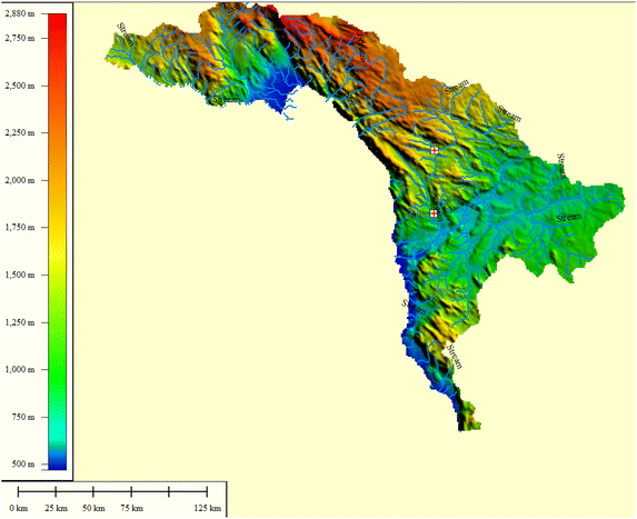
Surface elevation (top of layer 1). The cross line symbols represent two stream gauging stations
-
Layer 2: A non-uniform deep basement layer ranging in thickness from 400 m to 1500 m.

Boundary and initial conditions
For the purpose of modelling the basin, a simplified aquifer system has been used. The upper model layer is assumed to be one continuous interconnected aquifer with different permeability zones based on the geology. The initial potentiometric surface (Fig. 7) was estimated from borehole data where a water level and location were available. The groundwater elevation was estimated using the borehole location and digital elevation model.

Potentiometric surface of Lake Nyasa basin. The basin is shown as the dashed red line and blue dots represent boreholes with water levels
Recharge and discharge
Recharge is assumed to be predominantly from rainfall infiltration. This may occur as direct recharge through exposed bedrock fractures or via slow percolation through the weathered overburden. A small component of recharge is thought to occur via stream and river bed leakage especially in the lower reaches of the river systems. As there is no long term water level monitoring data recharge has been assumed to be a percentage of the total annual rainfall [39]. Rainfall infiltration rates in the order of 5–20% have been estimated during the model calibration. Recharge zoning was made based on the geology and rainfall isohyet map.
Groundwater discharge is via evapotranspiration, baseflow of streams and rivers (as river leakage which discharges to the Lake), pumping, and deep percolation discharge to Lake Nyasa. The component of deep percolation is generally assumed to be about 10% of recharge. In the elevated plateaus of the catchments, baseflow is assumed to be the major discharge mechanism. In the lower reaches, evapotranspiration is thought to play a larger role especially in the lower reaches of the Ruhuhu River and Kyela alluvials. Given the depth of groundwater is generally shallow in the model area, the evapotranspiration (ET) is considered significant. The ET rate was set at 10% of the estimated values shown on Fig. 2, with an extinction depth of 2 m. The ET rate was refined during the calibration process.
Hydraulic parameters
Aquifer properties were set based on the limited available information and accepted literature values (e.g. [40]). The properties were further refined (within acceptable limits) during model calibration and the adopted values are provided in Table 1. Initial attempts to calibrate the model using a single zone for the upper layer were unsuccessful. Zoning the upper layer (Fig. 8) was required for calibration adding confidence to the approach.

Hydraulic conductivity zones used for the model calibration
The initial head was interpolated from limited water levels recorded is used as the starting point for model calibration. The interpolation was used to establish precalibration steady-state conditions.
Model calibration
An attempt has been made to reproduce the observed water levels in the entire study area through the steady model. The heads may have been reproduced, but the solution is nonunique. The numerical model includes assumptions based on literature values and the experience of the modeller due to the limited amount of hydrogeological data. Limitations exist with respect to the amount of water level data available to constrain the calibration and aquifer recharges rates and spatial distribution of recharge areas. Calibration was accomplished by applying a set of hydraulic parameters; boundary conditions and stresses that produce computer generated simulated hydraulic heads that match actual field measurement within an acceptable range of error. Model calibration was performed using manual (trial and error) methods. The model was calibrated using observed groundwater heads and processed baseflow estimate. To improve calibration, the hydraulic conductivity, recharge and river conductance were adjusted until the modelled head elevations were able to match observed head elevations to an acceptable level of accuracy with a correlation coefficient of 0.97. The root mean squared error and residual mean error are 1.6 and −0.66 m respectively. This indicates a good correlation between observed and calculated groundwater heads [41, 42]. Analysis of the calibrated steady state model output indicates that the model simulates the groundwater elevation, hydraulic gradient and flow direction (Fig. 9) across the active model area to an acceptable level. The model calibration is considered acceptable, considering the correlation coefficient, mass balance 0.0% discrepancy) (Table 2) and spatially random residual errors [41, 43]. Sensitivity analysis carried out prior to steady state model calibration showed that the recharge flux parameter and hydraulic parameter of top layer are most sensitive.

Steady state calibrated potentiometric surface for layer 1
Processed baseflow
Baseflow measurements in streams and rivers may be used as additional calibration targets as they allow calibrating to a flow rate as a head distribution, which may greatly increase the uniqueness or confidence of the model calibration. For this study, stream flow measurements from two locations on the Kitiwaka River recorded during an extended dry period on the 16th December 1983 were selected for the analysis (indicated by a cross line symbol on Fig. 6). The difference between these flow measurements is the net baseflow to the stream, assuming evaporative losses are negligible.
Results and discussion
Simulated water balances
Based on the results of the simulation, the water balances were studied in the entire basin of the study area, to understand the functioning of the aquifers and their relationship with the Lake Nyasa. The aquifer is highly influenced by the diffuse recharge, which causes the water balances to change rapidly from positive to negative. The total water inflow (calculated as the sum of the net river/streambed recharge, the diffuse recharge and the lateral inflow) fluctuates greatly, due to climate variability. However, the total outflow (calculated as the sum of the evapotranspiration, outflow towards Lake Nyasa and the river leakage) remains practically stable. This fact is because the volume abstracted is nill or small compared to the total volume exchanged with basin, which is almost constant over time and is independent of the climate or of the aquifer exploitation (Table 2). Given that any surplus or deficit causes a change in the groundwater storage, and if it is assumed that the predevelopment pseudo-stationary state defines the equilibrium for the aquifer storage, the evolution can be observed of the accumulated deficits expected in the Lake Nyasa basin. However, The Lake Nyasa basin can exhibit the opposite behaviour. The total outflow term may be highly dependent on the total volume abstracted, while total inflows are less variable than in the case of the Lake Nyasa. Moreover, the inverse effect is expected if the water rights are not used, due to the importance of the streambed recharge (Table 3). The expected behaviour of these hydrogeological units, therefore, is clearly dependent upon the total abstraction.
The net flow across the river boundary is calculated as follows:
A negative result indicates a net loss of water from the aquifer to the Kitiwaka River as all flow rates in MODFLOW are considered with respect to the aquifer. The recorded gain in net flow is 2.05 m3/day while the model indicates a gain of 1.85 m3/day. The difference (0.2 m3/day) is small (~90% similarity) and well within the error of the model. The model result indicates that net loss of water from the aquifer may explain ~88% of the difference in stream flow between the two stream flow gauge stations. This is in agreement with the estimated baseflow component processed using baseflow Index [34] method (i.e. 85%).
Volumetric budget for each catchment
The water balance for each catchment (Table 4) was computed using the Zone-budget software package [44]. Zone-budget is a program that computes the water budget for a designated zone using results from the MODFLOW-SURFACT groundwater flow model (Zone budget-version 3.01, updated year 2009). The Zone budget is a tool for measuring the flow from one part of the model to another. The zone budget was employed to create a baseflow measurement zone along Kitiwaka River, between the two stream gauging stations. This allows assessment of the gain or loss of stream flow. The measured and predicted baseflow values were then compared and the model parameters adjusted to improve the model calibration.
The two stream gauging stations located along the Kitiwaka River are indicated by a cross line symbol on Fig. 6. The measured stream flow at the downstream station was about 2.33 m3/day and at the upstream station it was 0.28 m3/day. The difference between these two numbers represents the river gain or water coming from the groundwater system and can be compared with the flow across the river boundary calculated by zone budget. To examine the amount of groundwater flow between the stream and the aquifer system, the river leakage under the input and output columns were extracted from the model output (Table 4).The projected population (Table 5), will likely have an impact on the estimated volumetric water budget.
Annual safe yield/extraction limit
Based on the model the average net recharge and water in storage has been estimated (Table 6). In the absence of long term monitoring data to assess the performance of the aquifers the annual safe yield can be expressed as a percentage of the annual recharge [45]. Globally, if recharge can be assumed to be approximately 20% of precipitation, then deep percolation would be about 10% of recharge. Thus, a reasonably conservative estimate of sustainable yield would be 10% of the net recharge. The current concept of sustainable yield represents a compromise between theory and practice. In theory, a reasonably conservative estimate of sustainable yield would be about 10% of recharge. In practice, values higher than 10% may reflect the need to consider other factors besides conservation. Turner et al. [14] concluded that an aquifer system sustained by episodic recharge and the long-term gaining storage represents the maximum extractable volume.
To assess the potential groundwater resource for the basin the recharge has been estimated using the groundwater model. The estimated sustainable safe yields from the groundwater model for each catchment are compared to the estimated current domestic groundwater usage with a 20% contingency added for stock watering, small scale irrigation, commercial, institution (schools and Government buildings) and losses. Industrial, Mining and large scale agriculture are not included, they are considered socio-economic demands which may be developed after domestic uses are covered. It can be seen (Table 6) that currently the percentage of annual safe yield extracted ranges between 6.8 and 62%, averaging around 29%. This suggests there is room for socio-economic expansion of groundwater usage within all catchments.
The annual safe yield of the basin is taken as 10% of the total annual recharge and calculated to be 10.7 × 10⁷ m3. Current conservative estimates of groundwater use within the basin are around 27.3 × 10⁵ m3 which is around 30% of the basin annual safe yield. The current catchment groundwater usage ranges between 10 and 60% of the annual safe yield leaving between 90 and 40% of the annual safe yield depending on sub catchment available for future development [46]. Based on the current model result, estimate of groundwater recharge for the study area is about 1.07 × 10⁶ m3/day. Thus, the limits on aquifer pumping as a percentage of groundwater recharge range can be computed for the sustainable yield. Elsewhere, a value of total use of 50–70% of the sustainable yield was adopted.
Future scenario
Future predictions of groundwater usage and the resulting percentage of the annual safe yield used are provided in Table 7. In recent years, hydrological models, with various degrees of sophistication, have been used in various settings to evaluate water budgets for sustainable yield estimate under various climate or land-use scenarios (e.g. [11, 47]).
Impacts on groundwater due to the population patterns may include increased abstraction for domestic, industrial or agricultural purposes, decreased recharge through land clearing and urbanisation, contamination from sewage and chemicals and localise increases in recharge due to storm water soakaway’s in urban areas. Population concentrations in areas with limited access to gravity schemes, such as the south eastern part of Ruhuhu catchment near Songea, have resorted to groundwater for domestic water supplies.
These predictions do not account for possible reductions in the total annual recharge as a result of climate change [48]. It can be seen that by 2035 the percentage of annual safe yield extracted will increase to between 11.3 and 103%, averaging around 50%. This indicates that less water may be available for socio-economic development in the future. It also suggests that by 2035 Kiwira and Mbaka sub catchments will be nearly at or exceeding the annual safe yield leaving no room for socio-economic development, or the need to reduce existing socio-economic demands to meet domestic demands. The other option is to increase the percentage of total recharge allocated to the annual safe yield from 10 to 20% in these catchments.
Basin sustainability yield constraints
The current study shows that derivation of sustainable yield using conservation of mass principles leads to expressions for basin sustainable that can be readily determined using numerical modeling methods and selected on the basis of applied constraints. Bores are concentrated in areas of high population. For instance the village of Mlete, in Tanga Ward, Namtumbo District has 21 identified bores. The yield from each bore may not be high, but the combined yield of all 21 bores may be. Viewed on a large scale this is likely not an issue, however the combined yield of the bores may exceed the safe yield in a small area leading to localised drawdown.
The possibilities of severe, long-term droughts and climate change also should be considered. Because a climate stress on the hydrologic system is added to the existing or projected human-derived stress, droughts represent extreme hydrologic conditions that should be evaluated in any long-term management plan. Water reuse is one of the potential ways to complement the existing portable water sources. Practice of the water reuse for irrigation in Tanzania and similar region has been suggested by Kihila et al. [28]; Yihdego [49]. The challenges that need to be addressed, the benefits expected and global wastewater treatment options, capital and operation costs as well as the cost benefit analysis, implementation of water reuse will require among other things, proper defined policy and institutional framework, clear guidelines as well as more research and investment on wastewater treatment have been pointed out [28].
Transboundary considerations
When considering the groundwater potential and annual safe yield for the basin the potential for Transboundary impacts must be considered. Lake Nyasa is shared between three countries while the basin borders three countries, Zambia and Malawi along the north western boundary marked by the Songwe River and Mozambique on the southern boundary (Fig. 1). The Songwe River marks the border of Tanzania with Zambia and Malawi, the river is gaining having a high groundwater baseflow. On the Zambia/Malawi side are high hills and mountains which fall towards the river indicating the groundwater flow direction is also towards the river. Extraction of groundwater within the basin (Tanzania) is unlikely to impact groundwater across the border and the potential for transboundary impacts are considered very low. However over extraction of groundwater may impact baseflow to the river and therefore surface flows in the river which may impact users on both sides of the border. The southern basin boundary with Mozambique is an arbitrary line which doesn’t follow topographic features, therefore there is a potential for transboundary impacts. However the length of border is short and in a mountainous area with high rainfall and low population limiting the potential for extraction. The potential for transboundary groundwater impacts are therefore considered low to very low.
Conclusions
To analysis the groundwater development based on sub-basin/sub-catchment, a three dimensional groundwater numerical modelling (MODFLOW-SURFACT coupled with Visual MODFLOW) were used to handle Vadose Zone and for greater numerical convergence stability. Groundwater modelling and water balance optimization were used for the sustainable yield estimation. The model has been calibrated to the hydraulic head and processed baseflow estimate, which adds confidence or none-uniqueness to the solution and hence as a basis good enough for prediction/scenario simulation. A water-budget model output was used in estimating recharge which allows for an evaluation of the future groundwater sustainability, with several sub-basin extraction limits/annual safe yields in the Lake Nyasa basin. The water balance error was 0% which could be considered as criteria (i.e. water balance stabilization), to constrain the estimate of sustainable extraction [13]. Based on the current model result, estimate of annual safe yield based on 10% of groundwater recharge for the study area is about 10.7 × 10⁷ m3. The current catchment groundwater usage ranges between 10 and 60% of the annual safe yield leaving between 90 and 40% of the annual safe yield, depending on sub catchment, available for future development. Future predictions of groundwater usage indicate that by 2035 the percentage of annual safe yield extracted will increase to between 11.3 and 103%. Sustainability indicators such as acceptable head can be examined based on climate and management decisions affecting water extraction and land use. The choice of the method employed in this study has proved successful for a sound understanding of the sub-basin groundwater resources sustainability among the stake holders, decision makers for an effective management. With this information, society can make better informed decisions about how to manage their ground water resources in a long-term context. Such analyses also ideally lead to the design and implementation of long-term hydrologic networks to monitor projected outcomes of the ground water development and to improve the ability to predict future system responses.
The basin size is relatively small and annual groundwater recharge volumes are low, assuming between 5 and 20% of rainfall and therefore sustainable groundwater extraction volumes will be low, and there is insufficient information to assess the component of deep circulation and hence the deep groundwater resource within the fractured rock systems. The possibility of transboundary issues are considered low due to the prevailing groundwater gradient in the areas of international borders. It is more likely groundwater extraction may lead to reduced baseflows especially in the Songwe River which may impact surface water users on both sides of the border. Basin groundwater quality is generally good due to the annual recharge of the shallow aquifers. Based on the limited available groundwater analysis all aquifer types in all catchments may be suitable for domestic and stock watering purposes subject to assessment of individual bores.
The effect of few management options and a simplified climatic-change scenario needs to be considered for the Lake Nyasa sub-basin aquifers together with a decrease in the net recharge (and possibly suggest Managed Aquifer Recharge/Aquifer Storage recovery), a change in river–aquifer interactions, and the total abstraction volumes identified as the main factors to address in management planning. Further efforts to constrain the hydrogeological parameters of the various geological units, including riverbed deposits, which could include targeted test pumping, could improve understanding of the system.
References
Al-Weshah R, Yihdego Y (2016) Modelling of strategically vital fresh water aquifers, Kuwait. Environ Earth Sci 75:1315. doi:10.1007/s12665-016-6132-1
Yihdego Y, Reta G, Becht R (2016) Human impact assessment through a transient numerical modeling on the UNESCO World Heritage Site, Lake Naivasha, Kenya. Environ Earth Sci. doi:10.1007/s12665-016-6301-2
Yihdego Y, Reta G, Becht R (2016) Hydrological analysis as a technical tool to support strategic and economic development: case of Lake Naivasha, Kenya. Water Environ J 30(1–2):40–48. doi:10.1111/wej.12162
Yihdego Y, Drury L (2016) Mine water supply assessment and evaluation of the system response to the designed demand in a desert region, central Saudi Arabia. Environ Monit Assess J 188:619. doi:10.1007/s10661-016-5540-8
Ozdemir A (2011) GIS-based groundwater spring potential mapping in the Sultan mountains (Konya, Turkey) using frequency ratio, weights of evidence and logistic regression methods and their comparison. J Hydrol 411:290–308
Pourtaghi ZS, Pourghasemi HR (2014) GIS-based groundwater spring potential assessment and mapping in the Birjand Township, southern Khorasan Province, Iran. Hydrogeol J 22(3):643–662
Bredehoeft J (2005) The conceptualization model problem: surprise. Hydrogeol J 13:37–46
Alley WM, Leake SA (2004) The journey from safe yield to sustainability. Ground Water 42:12–16
Devlin JF, Sophocleous M (2005) The persistence of the water budget myth and its relationship to sustainability. Hydrogeol J 13:549–554
Sophocleous M (2000) From safe yield to sustainable development of water resources: the Kansas experience. J Hydrol 235:27–43
El-Kadi AI, Tillery S, Whittier RB, Hagedorn B, Mair A, Ha K, Koh G (2014) Assessing sustainability of groundwater resources on Jeju Island, South Korea, under climate change, drought, and increased usage. Hydrogeol J 22(3):625–642
Holman IP, Tascone D, Hess TM (2009) A comparison of stochastic and deterministic downscaling methods for modelling potential groundwater recharge under climate change in East Anglia, UK: implications for groundwater resource management. Hydrogeol J 17:1629–1641
Smith A, Walker G, Turner J (2010) Aquifer sustainability factor: a review of previous estimates. International Association of Hydrogeologists (AIH) and the Geological Society of Australia (GSA). EP104589
Turner RJ, Mansour MM, Dearden RÓ, Dochartaigh BÉ, Hughes AG (2015) Improved understanding of groundwater flow in complex superficial deposits using three-dimensional geological-framework and groundwater models: an example from Glasgow, Scotland (UK). Hydrogeol J 23:493–506
Whittier R, Rotzoll K, Dhal S, El-Kadi AI, Ray C, Chang D (2010) Groundwater source assessment program for the state of Hawaii, USA: methodology example application. Hydrogeol J 18:711–723
Conan C, de Marsily G, Bouraoui F, Bidoglio G (2003) A long-term hydrological modelling of the Upper Guadiana river basin (Spain). Phys Chem Earth 28:193–200
Bromley J, Cruces J, Acreman M, Martínez L, Llamas MR (2001) Problems of sustainable groundwater management in an area of over-exploitation: the upper Guadiana catchment, central Spain. Int J Water Resour Dev 17:379–396
Martínez-Santos P, Llamas MR, Martínez-Alfaro PE (2008) Vulnerability assessment of groundwater resources: a modelling-based approach to the Mancha Occidental aquifer, Spain. Environ Model Softw 23:1145–1162
Yihdego Y, Danis C, Paffard A (2015) 3-D numerical groundwater flow simulation for geological discontinuities in the Unkheltseg Basin, Mongolia. Environ Earth Sci J 73(8):4119–4133
Yihdego Y, Becht R (2013) Simulation of lake–aquifer interaction at Lake Naivasha, Kenya using a three-dimensional flow model with the high conductivity technique and a DEM with bathymetry. J Hydrol 503:111–122
Carrera J, Alcolea A, Medina A, Hidalgo J, Slooten LJ (2005) Inverse problem in hydrogeology. Hydrogeol J 13:206–222
Yihdego Y, Webb JA (2011) Modeling of bore hydrograph to determine the impact of climate and land use change in a temperate subhumid region of south-eastern Australia. Hydrogeology Journal 19(4):877–887
Yihdego Y, Webb JA (2015) Use of a conceptual hydrogeological model and a time variant water budget analysis to determine controls on salinity in Lake Burrumbeet in southeast Australia. Environ Earth Sci J 73(4):1587–1600
Yustres A, Navarro V, Asensio L, Miguel Candel M, García B (2013) Groundwater resources in the Upper Guadiana (Spain): a regional modelling analysis. Hydrogeol J 21:1129–1146
Orr S, Meystel AM (2005) Approaches to optimal aquifer management and intelligent control in a multi-resolutional decision support system. Hydrogeol J 13:223–246
Danish International Development Agency (DANIDA) (1988) Implementation of water master plan for Iringa, Ruvuma and Mbaya regions, for United Republic of Tanzania
Don Consult Ltd (2011) Provision of technical and facilitation consultancy services for rural water supply and sanitation sub-projects in Kyela district council, exploration drilling report. Tender No: LW/DC/F. 10/15/Vol. V/108, July 2008. Report for the United Republic of Tanzania, Prime Minister’s Office Regional administration and Local Government, Water Sector Development Program
Kihila J, Mtei KM, Njau KN (2015) A review of the challenges and opportunities for water reuse in irrigation with a focus on its prospects in Tanzania. Int J Environ Eng 7(2):111–130. doi:10.1504/IJEE.2015.069817
SMEC (2013) Integrated water resources management and development plan—groundwater assessment. Ministry of Water, Dar es Salaam
Bootsma HA, Jorgensen SE (2006) Lake Malawi/Nyasa. Experience and lessons learned brief. http://Worldlakes.org. Accessed 25 March 2015
Kashaigili JJ (2010) Assessment of groundwater availability and its current and potential use and impacts in Tanzania, Report for International Water Management Institute, December 2010
Lake Nyasa Basin Water Board (LNBWB) (2010) Basin (Lake Nyasa) hydrological report, December 2010
Arnold JG, Allen PM, Muttiah R, Bernhardt G (1995) Automated baseflow separation and recession analysis techniques. Ground Water 33(6):1010–1018
Beck HE, Albert I, van Dijk JM, Miralles DG, de Jeu RAM, Bruijnzeel LA, McVica TR, Schellekens J (2013) Global patterns in baseflow index and recession based on stream flow observations from 3394 catchments. Water Resour Res 49(12):7843–7863
Smakhtin VU (2001) Estimating continuous monthly baseflow time series and their possible applications in the context of the ecological reserve. Water SA 27(2):213–218 (ISSN 0378–4738)
Howard AE (2011) A brief introduction to the geology and mining history of Tanzania. Report prepared for SIKA RESOURCES INC. Nebu Consulting LLC, Toronto
Hagedorn B, El-Kadi AI, Mair A, Whittier RB, Ha K (2011) Estimating recharge in fractured aquifers of a temperate humid to semiarid volcanic island (Jeju, Korea) from water table fluctuations, and Cl, CFC-12 and 3H chemistry. J Hydrol 409:650–662
HydroGeoLogic Inc (2002) MODFLOW-SURFACT: a comprehensive MODFLOW-based hydrologic modelling system: code documentation and user’s manual. HydroGeoLogic Inc, Reston
Sanz D, Castaño S, Cassiraga E, Sahuquillo A, Gómez-Alday J, Peña S, Calera A (2011) Modeling aquifer–river interactions under the influence of groundwater abstraction in the Mancha Oriental System (SE Spain). Hydrogeol J 19:475–487
Fetter CW (2001) Applied hydrogeology, 4th edn. Prentice Hall, Englewood Cliffs
Barnett B, Townley LR, Post V, Evans RE, Hunt RJ, Peeters L, Richardson S, Werner AD, Knapton A, Boronkay A (2012) Australian groundwater modelling guidelines, waterlines report. National Water Commission, Canberra
Knowling MJ, Werner AD, Herckenrath D (2015) Quantifying climate and pumping contributions to aquifer depletion using a highly parameterized groundwater model: Uley South Basin (South Australia). J Hydrol 523:515–530
Middlemis H (2004) Benchmarking best practice for groundwater flow modelling. The Winston Churchill Memorial Trust of Australia
Harbaugh AW (1990) Zone budget. A computer program for calculating subregional water budgets using results from the US geological survey modular three-dimensional ground-water flow model: US geological survey open-file report 90–392
Kalf FRP, Woolley DR (2005) Applicability and methodology of determining sustainable yield in groundwater systems. Hydrogeol J 13:295–312
Mair A, Hagedorn B, Tillery S, El-Kadi AI, Westenbroek S, Ha K, Koh GW (2013) Temporal and spatial variability of groundwater recharge on Jeju Island, Korea. J Hydrol 501:213–226
Fornés JM, De La Hera Á, Llamas MR (2005) The silent revolution in groundwater intensive use and its influence in Spain. Water Policy 7:253–268
Yihdego Y, Webb JA (2016) Validation of a model with climatic and flow scenario analysis: case of Lake Burrumbeet in southeastern Australia. J Environ Monit Assess 188(308):1–14. doi:10.1007/s10661-016-5310-7
Yihdego Y (2015) Water reuse and recreational waters, urban water reuse handbook (UWRH), chapter 78. In: Eslamian S. (ed) Taylor and Francis, CRC Press, Boca Raton, pp 1029-1039. Print ISBN: 978-1-4822-2914-1. eBook ISBN: 978-1-4822-2915-8. CAT# K22608. https://www.crcpress.com/Urban-Water-Reuse-Handbook/Eslamian/p/book/9781482229141
Authors’ contributions
YY performed numerical simulation and wrote most of the sections of the paper. AP analysed the field data and wrote some sections of the paper. All authors read and approved the final manuscript.
Acknowledgements
We acknowledge SMEC International and Tanzanian Ministry of Water. The study was funded by the International Development Association and the United Republic of Tanzania.
We would like to extend our thanks to Lake Nyasa Basin Water Board; Sokoine University of Agriculture, Tanzania; Drilling and Dams Construction Agency (DDCA), Dar es Salaam Office; Songea District Water Engineers Office, and Kyela District Water Engineers Office. The manuscript has benefitted from the reviewers’ and editors’ comments.
Competing interests
The authors declare that they have no competing interests.
Author information
Authors and Affiliations
Corresponding author
Rights and permissions
Open Access This article is distributed under the terms of the Creative Commons Attribution 4.0 International License (http://creativecommons.org/licenses/by/4.0/), which permits unrestricted use, distribution, and reproduction in any medium, provided you give appropriate credit to the original author(s) and the source, provide a link to the Creative Commons license, and indicate if changes were made.
About this article

Cite this article
Yihdego, Y., Paffard, A. Hydro-engineering solution for a sustainable groundwater management at a cross border region: case of Lake Nyasa/Malawi basin, Tanzania. Geo-Engineering 7, 23 (2016). https://doi.org/10.1186/s40703-016-0037-4
Published:
DOI: https://doi.org/10.1186/s40703-016-0037-4