A secular variation candidate model for IGRF-13 based on Swarm data and ensemble inverse geodynamo modelling

Abstract

This paper describes the design of a candidate secular variation model for the 13th generation of the International Geomagnetic Reference Field. This candidate is based upon the integration of an ensemble of 100 numerical models of the geodynamo between epochs 2019.0 and 2025.0. The only difference between each ensemble member lies in the initial condition that is used for the numerical integration, all other control parameters being fixed. An initial condition is defined as follows: an estimate of the magnetic field and its rate-of-change at the core surface for 2019.0 is obtained from a year (2018.5–2019.5) of vector Swarm data. This estimate (common to all ensemble members) is subject to prior constraints: the statistical properties of the numerical dynamo model for the main geomagnetic field and its secular variation, and prescribed covariances for the other sources. One next considers 100 three-dimensional core states (in terms of flow, buoyancy and magnetic fields) extracted at different discrete times from a dynamo simulation that is not constrained by observations, with the time distance between each state exceeding the dynamo decorrelation time. Each state is adjusted (in three dimensions) in order to take the estimate of the geomagnetic field and its rate-of-change for 2019.0 into account. This methodology provides 100 different initial conditions for subsequent numerical integration of the dynamo model up to epoch 2025.0. Focussing on the 2020.0–2025.0 time window, we use the median average rate-of-change of each Gauss coefficient of the ensemble and its statistics to define the geomagnetic secular variation over that time frame and its uncertainties.

Background

The International Geomagnetic Reference Field (IGRF henceforth) encapsulates three standard mathematical models of Earth’s magnetic field and is released by the International Association of Geomagnetism and Aeronomy (IAGA) every 5 years. One of these three mathematical models represents a forecast of the evolution of the main geomagnetic field for the 5 years to come, and it is referred to as the secular variation (SV) model. For the current release of the IGRF described in this special issue (Alken et al. 2020a), the 5-year window starts on January 1st, 2020 and ends on December 31st, 2024. The secular variation model is truncated at spherical harmonic degree 8; it rests on the assumption that each Gauss coefficient undergoes an independent linear evolution over the 5 years of interest. The linear interpolation of each Gauss coefficient between its adopted value in 2020.0 and any instant over that time interval will allow any end-user to compute the value of any geomagnetic element he or she is interested in during that period, at any location on Earth.

The latest version of the IGRF, hereafter referred to as the 13th generation of IGRF (IGRF-13), was released in December 2019 (Alken et al. 2020a). IPGP has been involved in a number of candidate models, notably the DGRF candidate by Vigneron et al. (2019), the IGRF candidate by Ropp et al. (2020), the SV candidate described here, in addition to the IGRF candidate by Yang et al. (2020) and the SV candidate proposed by Minami et al. (2020), all of which are presented in this special issue. A total of 14 international teams proposed candidate secular variation models, a substantial increase with regard to the 12th generation, to which eight teams contributed (Thébault et al. 2015). A task force appointed by IAGA assessed the quality of the candidate models and proposed a composite model based on those candidates (consult Alken et al. 2020b, in this issue to see how the evaluation has been carried out for IGRF-13).

The goal of this paper is to describe the secular variation candidate proposed by IPGP for IGRF-13. To forecast the evolution of the geomagnetic field until 2025, we combine geomagnetic data provided by the Swarm constellation (Olsen et al. 2013) with a physics-based model of the geomagnetic field, in the form of a numerical model of the geodynamo. This methodology, classically referred to as data assimilation, has been investigated for more than a decade in geomagnetism (e.g. Fournier et al. 2010; Wicht and Sanchez 2019). The applications of data assimilation to geomagnetism are fundamental (e.g. Gillet et al. 2010; Aubert 2015) and practical, a recent example of the latter being the forecast of the evolution of the low-altitude proton environment for the next few decades (Bourdarie et al. 2019). Another practical application of geomagnetic data assimilation is the one of interest here: it builds on our previous contribution to IGRF-12 (Fournier et al. 2015) and includes a few novelties, most notably an ensemble framework to approximate the uncertainties impacting the numerical dynamo model.

Methods

Here we describe first how we construct an “initial” model for year 2019.0 from Swarm data, and second how this initial model is used to initialize an ensemble of dynamo-based forecasts of the evolution of the main geomagnetic field from 2019.0 to 2025.0. This ensemble allows us to define a candidate secular variation model for IGRF-13 and its uncertainties.

Construction of the initial model for 2019.0

Data selection

We consider only vector data for Swarm satellite A (Alpha) from epoch 2018.5 to epoch 2019.5. We do not utilize magnetic intensity data. We use systematically the latest version of the data and select first the processed data (SW_OPER_MAGA_LR), then, depending on the epoch, either version 0505 (for the most part) or version 0506.

Data selection differs depending on the geomagnetic latitude. We distinguish high-latitude (HL henceforth) data from mid-latitude (ML henceforth) data. HL (resp. ML) data correspond to a geomagnetic latitude of absolute value larger (resp. smaller) than $55^\circ$.

The following selection criteria apply:

• ML data are selected for local times between 11:00 pm and 5:00 am, and rejected for sunlit ionosphere.

• Data are selected for positive values of the vertical component of the interplanetary magnetic field (IMF), $B_{IMF}^Z$: $B_{IMF}^Z > 0$.

• Data are further selected based on the $D_{st}$ index. The $D_{st}$ index, which measures the activity of the magnetic field generated by the ring current, is requested to have values in the $\left[ -30 : 30 \right]$ nT range.

• ML data are sampled every 30 seconds, while HL data are sampled every 60 seconds. Approximately, this corresponds to collecting one ML datum every two degrees and one HL datum every four degrees along the satellite track.

The size of the corresponding data vector ${\mathbf {d}}$ is $493,620\, (=3\times 164,540)$. The locations of the corresponding measurements are shown in Fig. 1. Note that HL data are handled in the usual North, East, Centre (NEC) reference frame, whereas ML data are used in a Solar Magnetic (SM) reference frame, in order to lower the correlations between vector data component errors (Lesur et al. 2008).

Fig. 1

The location of those measurements used to constrain the initial magnetic field model. Top: Mollweide projection. Bottom: orthographic projections centred on the North pole (left) and South pole (right). Every third point shown for clarity

Data weighting

The variances attributed to each type of data were chosen based on experience and they are given in Table 1. The inverse of the variance is used to weigh the data when constructing the initial model.

Table 1 Variances prescribed to the three components of mid-latitude (ML) and high-latitude (HL) vector data

Modelling method and initial model parameterization

The approach used to build this model is to fit data through a robust re-weighted iterative least-squares process, using Huber weights. The first iteration is a standard $L_2$-norm least-squares inversion.

The magnetic field potential V is represented using a spherical harmonic expansion of the form

$$\begin{aligned} V(r,\theta ,\varphi ,t)= & {} V_i(r,\theta ,\varphi ,t)+V_e(r,\theta ,\varphi ,t) \end{aligned}$$

(1)

$$\begin{aligned}= & {} a \sum _{\ell =1}^{L_i} \left( \frac{a}{r} \right) ^{\ell +1} \sum _{m=0}^{\ell } \left[ g_\ell ^m(t) \cos \left( m \varphi \right) + h_\ell ^m(t) \sin \left( m \varphi \right) \right] {{\mathcal {P}}}_\ell ^m \left( \cos \theta \right) \nonumber \\&+ a \sum _{\ell =1}^{{L_e}} \left( \frac{r}{a} \right) ^{\ell } \sum _{m=0}^{\ell } \left[ q_\ell ^m(t) \cos \left( m \varphi \right) + s_\ell ^m(t) \sin \left( m \varphi \right) \right] {{\mathcal {P}}}_\ell ^m \left( \cos \theta \right) , \end{aligned}$$

(2)

in which $(r,\theta ,\varphi )$ denote the standard spherical coordinates, t is time, a is the mean radius of the Earth ($a=6371.2$ km), $L_i$ is the truncation of the spherical harmonic expansion of the internal sources (g and h), and $L_e$ the truncation of the expansion of the external sources (q and s). The ${{\mathcal {P}}}_\ell ^m$ are the associated Legendre functions of degree $\ell$ and order m, whose normalization is subject to the Schmidt convention.

The description of internal and external sources is done according to the guidelines provided by Holschneider et al. (2016). The idea is essentially to over-parameterize the contribution of each source and to constrain the resulting parameters using physical prior information.

Prior information on the model components is provided through the description of a Gaussian model distribution characterized by a mean and a covariance matrix. For all model sources the mean is zero. For the main field and its secular variation, the covariance matrix is built based on the statistics of the numerical dynamo model (more on this below). For all other sources, as in Holschneider et al. (2016), the covariance matrix is defined in terms of a radius R and a scaling factor $\gamma$. The radius R is the one at which the source spectrum is flat, and the scaling factor $\gamma$ is set such that the energy level corresponds to the estimated contribution of the source to the measured signal. Depending on the source, the value of $\gamma$ is set by optimization, or empirically, or by relying on the energy spectrum of the source if it happens to be known. In spectral space, this methodology amounts to defining covariance matrices ${\mathbf {C}}=C_{\ell \ell '}^{mm'}$ of the form

$$\begin{aligned} C_{\ell \ell '}^{mm'} = \gamma \delta _{\ell \ell '}\delta _{mm'} \left( \frac{R}{a}\right) ^{2 \ell +4} \text{ for } \text{ internal } \text{ sources } \end{aligned}$$

(3)

and

$$\begin{aligned} C_{\ell \ell '}^{mm'} = \gamma \delta _{\ell \ell '}\delta _{mm'} \left( \frac{a}{R}\right) ^{2 \ell } \text{ for } \text{ external } \text{ sources, } \end{aligned}$$

(4)

where $\delta$ denotes the Kronecker delta. The pairs of $(\gamma ,R)$ listed below for the various sources are slightly modified with respect to those appearing in the analysis of Lesur et al. (2018).

Internal sources

The truncation applied for internal sources is $L_i=30$. The main (dynamo) field is described up to spherical harmonic degree 18, and so is its secular variation. The secular variation is assumed to be constant between 2018.5 and 2019.5, and consequently the Gauss coefficients to vary linearly with time over this time frame. The prior information used to constrain these Gauss coefficients is based on the multivariate statistics of a 70,000-year-long free run integration of the coupled Earth dynamo model by Aubert et al. (2013). This choice is motivated by the will to ensure consistency between the initial model and the forecast that is produced using the same numerical model (more on the forecast below).

The crustal field is expanded in spherical harmonic degree from degree 15 to degree $L_i=30$ (prior covariance properties: $R=6280.0\,\hbox {km}$, $\gamma =2.7\ 10^{-2}$ nT$^2$). A known crustal field (Lesur et al. 2013) is subtracted from the data for degrees 30 to 110.

The mantle field induced by the magnetospheric ring current is described up to spherical harmonic degree 3, and each of its spherical harmonic component is assumed to be proportional to the internal component of the $D_{st}$ index (prior covariance properties: $R=2 537$ km, $\gamma =1$).

External sources

The external sources considered are the following:

• A static external field in the Geocentric Solar Magnetospheric (GSM) coordinate system for the remote magnetosphere (prior covariance properties: $R=16 000$ km, $\gamma =5400$ nT$^2$).

• A static external field in the Solar magnetic (SM) coordinate system for the near magnetosphere (prior covariance properties: $R=6 900$ km, $\gamma =3.56$ nT$^2$).

• A time-varying external field dependent upon the external $D_{st}$ index (prior covariance properties: $R=16 000$ km, $\gamma =5.4$).

• A time-varying external field dependent on the Y-component of the IMF in the SM coordinate system (prior covariance properties: $R=6 900$ km, $\gamma =0.1$).

Each of these external sources is described up to spherical harmonic degree $L_e=3$.

The initial model

The prior information on Gauss coefficients and their sources described above is encapsulated in a covariance matrix ${\mathbf {C}}_y$. If ${\mathbf {y}}_i$ denotes the vector of unknown Gauss coefficients after iteration i, iterations are governed by

$$\begin{aligned} {\mathbf {y}}_{i+1} = {\mathbf {y}}_{0} + \left( {\mathbf {A}}^T {\mathbf {W}}_i {\mathbf {A}} +{\mathbf {C}}_y^{-1}\right) ^{-1} {\mathbf {A}}^T {\mathbf {W}}_i \left( {\mathbf {d}} - {\mathbf {A}} {\mathbf {y}}_0 \right) , \end{aligned}$$

(5)

where ${\mathbf {A}}$ and ${\mathbf {W}}_i$ are the design and weight matrices, respectively. While the former is constant, the latter, ${\mathbf {W}}_i$, is updated at each iteration according to the re-weighting scheme described by, e.g. Farquharson and Oldenburg (1998). Since the initial vector of Gauss coefficients is filled with zeros, ${\mathbf {y}}_{0}={{\mathbf {0}}}$, and the previous equation simplifies to

$$\begin{aligned} {\mathbf {y}}_{i+1} = \left( {\mathbf {A}}^T {\mathbf {W}}_i {\mathbf {A}} +{\mathbf {C}}_y^{-1}\right) ^{-1} {\mathbf {A}}^T {\mathbf {W}}_i {\mathbf {d}} . \end{aligned}$$

(6)

The converged mean initial model, centred on 2019.0, is obtained after 3 iterations. The corresponding posterior covariance matrix ${\mathbf {C}}^{\text{ obs }}$ reads

$$\begin{aligned} {\mathbf {C}}^{\text{ obs }} = \left( {\mathbf {A}}^T {\mathbf {W}} {\mathbf {A}} +{\mathbf {C}}_y^{-1}\right) ^{-1}, \end{aligned}$$

(7)

where we understand that ${\mathbf {W}}$ contains the final weights. We can sketch its block-structure according to

$$\begin{aligned} {\mathbf {C}}^{\text{ obs }} = \left[ \begin{array}{lcccr} {\mathbf {C}}_{\textsc {mf}}^{\text{ obs }} &{} {\mathbf {C}}_{\textsc {mf}\leftrightarrow \textsc {sv}}^{\text{ obs }} &{} \cdots &{} \cdots &{} \cdots \\ {\mathbf {C}}_{\textsc {sv}\leftrightarrow \textsc {mf}}^{\text{ obs }} &{} {\mathbf {C}}_{\textsc {sv}}^{\text{ obs }} &{} \ddots &{} &{} \vdots \\ \vdots &{} \ddots &{} {\mathbf {C}}_{\textsc {crust}}^{\text{ obs }} &{} \ddots &{} \vdots \\ \vdots &{} &{} \ddots &{} \ddots &{} \ddots \\ \vdots &{} \dots &{} \dots &{} \dots &{} {\mathbf {C}}_{\textsc {imf}}^{\text{ obs }} \\ \end{array} \right] . \end{aligned}$$

(8)

Matrices on the diagonal express the confidence one should place in the sets of Gauss coefficients associated with each (internal or external) source. Of particular interest for what follows are ${\mathbf {C}}_{\textsc {mf}}^{\text{ obs }}$ and ${\mathbf {C}}_{\textsc {sv}}^{\text{ obs }}$, which quantify the uncertainties of the main field (MF) and the secular variation (SV) of the mean model at epoch 2019.0. We shall refer to this mean model for 2019.0 as our “initial” model henceforth. Off-diagonal matrices describe the covariances between different sets of coefficients. They are not explicitly shown in our sketch, save for matrices ${\mathbf {C}}_{\textsc {mf}\leftrightarrow \textsc {sv}}^{\text{ obs }}$ and ${\mathbf {C}}_{\textsc {sv}\leftrightarrow \textsc {mf}}^{\text{ obs }}$ which express the covariances between the main field and secular variation coefficients. We will not consider these in the following, given the sequential nature of the inverse modelling framework to be described below.

Note that the fit to the data (weighted by the Huber weight to data ratio) for the initial model is 1.31 nT. The axisymmetric field lines of the initial field model are shown in Fig.  2.

Fig. 2

A sketch of our workflow. Left panel: the initial magnetic field model for epoch 2019.0 ${{\mathbf {B}}}^{\text{ obs }}$ is estimated based on one year of Swarm data. This panel shows field lines of the axisymmetric meridional component of ${{\mathbf {B}}}^{\text{ obs }}$. The thick black lines correspond to the Earth’s surface, the core–mantle boundary and the inner-core boundary. Middle panel: the information on ${{\mathbf {B}}}^{\text{ obs }}$ is used together with the statistics of the coupled Earth dynamo model to estimate an ensemble of dynamo states for 2019.0. Shown is the radial magnetic field at the core–mantle boundary for a few members of the ensemble, with a zoom on ensemble member 43. For this ensemble member, an additional meridional slice comprises the axisymmetric meridional field lines on the right, and the axisymmetric toroidal field inside the core on the left, with a scale ranging from $-2$ mT (red) to $+2$mT (blue). Right panel: each dynamo state is advanced in time until 2025.0. The 100 trajectories so obtained are used to estimate the average secular variation between 2020.0 and 2025.0

Ensemble inverse geodynamo modelling

Our approach is similar to the one followed for our contribution to IGRF-12 (Fournier et al. 2015). Our workflow is tentatively summarized in Fig.  2. With the initial model (and its error covariance matrices ${\mathbf {C}}_{\textsc {mf}}^{\text{ obs }}$ and ${\mathbf {C}}_{\textsc {sv}}^{\text{ obs }}$) at hand, we apply the inverse geodynamo modelling framework of Aubert (2015), based on the coupled Earth dynamo (Aubert et al. 2013), with a few novel features, namely an ensemble approach to deal with uncertainties and the possibility to enforce a QG-MAC force balance at the core surface for the initial condition to be prescribed (Aubert 2020). The acronym QG-MAC stands for Quasi-Geostrophic Magneto-Archimedean-Coriolis and defines the hierarchical force balance estimated to prevail in Earth’s core (Aubert et al. 2017): a dominant geostrophic balance between the pressure gradient and the Coriolis force, followed at the next order of importance by a triple balance between the ageostrophic Coriolis force (the remainder of the Coriolis force not balanced by the pressure gradient), the buoyancy force and the magnetic force; consult Schwaiger et al. (2019) for a systematic study of the force balance in numerical dynamo simulations.

The multistep approach can be summarized as follows:

• (1) $N_e=100$ decorrelated independent dynamo states are extracted from a 70,000-year-long free run integration of the coupled Earth Dynamo.

• (2) For each ensemble member e, a Kalman filter estimates the three-dimensional structure of the magnetic field ${{\mathbf {B}}}^{\text{ dyn }}_e$ in the core interior from the field provided by the initial model ${{\mathbf {B}}}^{\text{ obs }}$ and the prior information based on the statistics (mean and covariance) of the 70,000-year-long free run integration. This step is referred to as the “Initialization” stage in Fig.  2. For more details regarding this step, and in particular the correlations between the magnetic field at the core surface and in its interior provided by the prior statistics, the interested reader is referred to the Appendix of Fournier et al. (2015). Figure 3 shows how the magnetic variance of the ensemble is impacted by this Kalman step. The variance is defined according to

  $$\begin{aligned} \mathrm {var}_{{\mathbf {B}}}(r) = \frac{1 }{N_e-1} \sum _{e=1}^{N_e}\overline{ \left[ {{\mathbf {B}}}^{\text{ dyn }}_e(r) - \overline{\langle {{{\mathbf {B}}}^{\text{ dyn }}}\rangle }(r)\right] ^2}, \end{aligned}$$

  (9)

  in which $\overline{\cdot }$ and $\langle {\cdot }\rangle$ denote spherical and ensemble averaging, respectively. Inspection of Fig.  3 reveals several important properties: before and after Kalman filtering, the variance is maximum on the fluid side of the interface between solid and liquid core regions, an indication of the active dynamics in this area, where plumes are initiated as this boundary layer is destabilized, and shear occurs between the solid inner core and the fluid outer core, leading to strong, time-dependent azimuthal fields. Also, the variance decreases almost linearly over the top 300 km of the core, an indication of the decrease of the strength of the toroidal field. Kalman filtering preserves the native trend of the ensemble, while leading to a decrease of the variance. The variance reduction is largest in the topmost 50 km of the core.

• (3) For each ensemble member e, the knowledge of the three-dimensional magnetic structure inside the core makes it possible to compute the three-dimensional magnetic diffusion vector inside the core, ${{\mathbf {D}}}^{\text{ mag }}_e$.

• (4) We next solve a diffusion-free core-flow problem at the core surface, seeking the core surface flow ${{\mathbf {u}}}_{s,e}$ which satisfies

  $$\begin{aligned} \hat{{{\varvec{r}}}}\cdot \left( \dot{{{\mathbf {B}}}}^{\text{ obs }} - {{\mathbf {D}}}^{\text{ mag }}_e \right) = -{{\varvec{\nabla }}}_h \cdot \left( {{\mathbf {u}}}_{s,e}\, \hat{{{\varvec{r}}}} \cdot {{\mathbf {B}}}^{\text{ dyn }}_e\right) , \end{aligned}$$

  (10)

  where ${{\varvec{\nabla }}}_h \cdot$ is the horizontal divergence and $\hat{{{\varvec{r}}}}$ is the unit vector in the spherical radial direction. This problem is solved under the weak constraint that the QG-MAC balance is satisfied at the core surface (Aubert 2020), in order for the resulting acceleration to remain in the range spontaneously exhibited by the coupled Earth model while preserving an adequate fit to the data—this is the mid-constraint option described by Aubert (2020).

• (5) Finally, another Kalman filter converts this estimate of ${{\mathbf {u}}}_{s,e}$ into a three-dimensional estimate of the flow and buoyancy fields, for this member of the ensemble.

  Fig. 3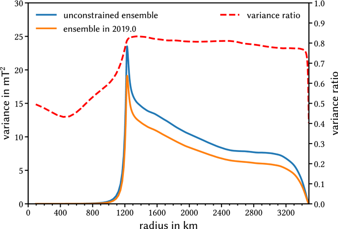

  

  Magnetic variance versus radius, for the 100 dynamo states before and after the assimilation of geomagnetic observations. The unconstrained ensemble refers to 100 decorrelated independent dynamo states extracted from a 70,000-year-long free run integration of the coupled Earth Dynamo. The ensemble in 2019.0 is obtained after applying a Kalman filter to adjust the magnetic field in the core interior for each ensemble member, given the constraints provided by the initial field model constructed at epoch 2019.0 from one year of Swarm data. The variance ratio is the ratio of the variances of the adjusted ensemble to the unconstrained ensemble

Note that this sequence of operations is performed using a spherical harmonic truncation of degree and order 30, which suffices to take the unmodelled secular variation into account, as ${{\mathbf {B}}}^{\text{ obs }}$ and $\dot{{{\mathbf {B}}}}^{\text{ obs }}$ are both truncated at spherical harmonic degree 13 (Aubert 2015, 2020). The three-dimensional estimates of the buoyancy, magnetic field and flow define a unique initial condition for the integration of the numerical dynamo model, details of which can be found in the study of Aubert et al. (2013) (and references therein). This integration is performed for each ensemble member e at the native resolution of the CE dynamo (maximum spherical harmonic degree and order 133). This implies that kinetic and magnetic energy beyond spherical harmonic degree 30 get progressively enriched by virtue of the nonlinearities of the dynamo system. This forecast stage is referred to as the “Forward Integration” step in Fig.  2. Inspection of Fig.  2 reveals small changes in the magnetic field structure of each ensemble member between 2019.0 and 2025.0.

Results and discussion

Before we introduce our candidate SV model, let us provide the reader with additional information with regard to the error budget and the steady flow assumption we decided to make.

Error budget and steady flow assumption

As noted in our 2015 study (Fournier et al. 2015), the methodology presented here “leaves in principle no room for tuning parameters, save for the scheme through which non-dimensional numerical dynamo quantities are cast into the dimensional world (for this last point, we use robust physical laws presumed to hold both in the numerical models and the Earth’s core (e.g. Aubert et al. 2013; Fournier et al. 2011)).” Yet at that time we had to address two issues: the first was connected with the error budget in the core-flow problem, and our interpretation was that it originated from the small size of the elements of the covariance matrix of the secular variation model, ${\mathbf {C}}_{\textsc {sv}}^{\text{ obs }}$. The second was connected with the statistical (as opposed to dynamical) nature of the initial dynamo state, which resulted in instabilities detrimental to the quality of the forecast.

Error budget

Values of the standard deviations for the initial secular variation model were on the order of $0.02-0.05$ nT/year for the large-scale components in our IGRF-12 study, a low value which may not reflect the fact that unmodelled external field variations can induce internal errors, and also that induced fields may not be adequately taken into account. In other words, an incomplete representation of non-orthogonal sources can lead to overestimate the accuracy of the modelled secular variation of the main field. In Fournier et al. (2015), we found it preferable to uniformly inflate ${\mathbf {C}}_{\textsc {sv}}^{\text{ obs }}$ in order to enhance the compatibility of the initial field model with the statistics of the coupled Earth dynamo. That amounted to a tenfold increase of the standard deviations of the secular variation coefficients. If we define the normalized misfit ${\mathcal {J}}_{\small {\textsc {sv}}}$ of the core-flow problem as

$$\begin{aligned} {\mathcal {J}}_{\small {\textsc {sv}}} = \sqrt{ \frac{1}{N_{{\small {\mathbf {y}}}}} \left( \widehat{{\mathbf {y}}}_{\small {\textsc {sv}}} - {\mathbf {y}}^{o}_{\textsc {sv}}\right) ^T \left( {\mathbf {C}}_{\textsc {sv}}^{\text{ obs }} \right) ^{-1} \left( \widehat{{\mathbf {y}}}_{\small {\textsc {sv}}} - {\mathbf {y}}^{o}_{\textsc {sv}}\right) }, \end{aligned}$$

(11)

where $\widehat{{\mathbf {y}}}_{\small {\textsc {sv}}}$ and ${\mathbf {y}}^{o}_{\textsc {sv}}$ are the vectors containing the $N_{{\small {\mathbf {y}}}}=195$ Gauss coefficients of the estimated secular variation and that of the initial model, respectively, the inflation allowed the normalized misfit to decrease from an initial value of 3.6 to 1.0.

For our IGRF-13 candidate, the large-scale diagonal coefficients of ${\mathbf {C}}_{\textsc {sv}}^{\text{ obs }}$ are such that they imply standard deviations on the order of 0.02–0.04 nT/year. These values are similar to the ones discussed above for our IGRF-12 candidate, in spite of the distinct methodology we followed to design the initial model. Again, these low values underestimate internal errors due to unmodelled external sources on the one hand and an inadequate representation of induced fields on the other hand. In fact, these large-scale low values are entirely data-driven, as the large-scale standard deviations of the coupled Earth SV Gauss coefficients (which are used to build the initial field model in order to ensure consistency) are ${\mathcal {O}}(1)$ nT/year. Yet, we did not inflate ${\mathbf {C}}_{\textsc {sv}}^{\text{ obs }}$ this time. The normalized misfit we get without inflation is equal to 2.2 (taking the ensemble mean for $\widehat{{\mathbf {y}}}_{\small {\textsc {sv}}}$), a value we consider acceptable. We propose two explanations to this lower value of ${\mathcal {J}}_{\small {\textsc {sv}}}$:

• In 2015, our initial model centred in 2014.3 was not regularized; this led to a very energetic SV at intermediate scales, even more so at the core–mantle boundary, where the core-flow problem is solved. By virtue of its design, our initial model centred in 2019.0 is less energetic at those scales, and more compatible with the Coupled Earth dynamo prior.

• Using an ensemble in step 4 above increases the compatibility between the dynamo and the initial SV model. The core-flow problem is solved for each ensemble member e as opposed to the ensemble mean. Each member corresponds to a fully saturated dynamo state, with a meaningful representation of intermediate to subgrid-scales. The ensemble mean, on which our 2015 approach was based, is under-energetic at these scales, which makes it harder to fit the SV model. Figure  4 illustrates the situation from an energetic standpoint, before the core–flow problem is solved. The black envelope is the one that would correspond to the approach we followed for IGRF-12, taking the mean and the statistics from the Coupled Earth dynamo. This tight envelope hardly intersects the blue envelope (that of the initial model), especially at large scales. Using an ensemble (thin red spectra) provides a broader range of possibilities which is beneficial to the overall scheme, once the mean (or the median) of the ensemble is considered, as will be demonstrated quantitatively in the next paragraph where the results of forecast-in-the-past experiments are presented.

Fig. 4

Secular variation spectra at the Earth’s surface. Each thin red line corresponds to an ensemble member, prior to the ingestion of the initial model for 2019.0. The blue envelope is that defined by the initial model plus or minus one standard deviation. In black, the envelope defined by the mean of the ensemble plus or minus one standard deviation

The steady flow assumption

The statistical (as opposed to dynamical) nature of the initial dynamo state for each ensemble member e leads to instabilities (i.e. unwanted flow accelerations) that are detrimental to the quality of the forecast, even when the QG-MAC balance is mildly enforced, according to the methodology described by Aubert (2020). Considering the evolution equation for the secular acceleration

$$\begin{aligned} \ddot{{{\mathbf {B}}}} = {{\varvec{\nabla }}} \times \left( \dot{{{\mathbf {u}}}} \times {{\mathbf {B}}} \right) +{{\varvec{\nabla }}} \times \left( {{\mathbf {u}}} \times \dot{{{\mathbf {B}}}} \right) +\frac{1}{\mu _0 \sigma } {{\varvec{\nabla }}}^2 \dot{{{\mathbf {B}}}}, \end{aligned}$$

(12)

in which $\sigma$ is the electrical conductivity and $\mu _0$ the magnetic permeability of vacuum, Christensen et al. (2012) demonstrated that in numerical dynamo simulations, the ${{\varvec{\nabla }}} \times \left( \dot{{{\mathbf {u}}}} \times {{\mathbf {B}}} \right)$ term is responsible for the low-degree ($\ell \le 10$) secular acceleration, thereby confirming the analysis of Lesur et al. (2010) based on co-estimated core field and flow models. Errors in this term can therefore have a large impact at the surface of the Earth. Assuming that the flow is steady over the forecast window is a conservative option. We assessed the validity of this assumption by performing forecast-in-the-past experiments, over the following time windows: 2005.0–2010.0, 2009.0–2014.0, 2015.0–2019.3. Note that for these three time intervals, the initial model based on satellite data fed to the dynamo ensemble (at epochs 2005.0, 2009.0 and 2015.0) was constructed according to the same protocol as the one used to construct the initial model for 2019.0 and detailed above. In addition, in order to assess the effect of each of the novelties introduced for IGRF-13 (the ensemble approach and the mild enforcement of the QG-MAC constraint), we considered the outcome of experiments conducted with or without these new features.

We begin by making some general remarks about the temporal and spectral behaviour of the error in those experiments we conducted using our framework. The error appears to grow quadratically with time over the time window of interest. In other words, it is during the last year of the forecast that most of the error is created (typically a third of the error at the end of the time window is generated during the last year of forecast). Considering now how the error is distributed as a function of spherical harmonic degree $\ell$, we find that spherical harmonic degrees $\ell =2,$ 3,  and 4 are the main contributors to the error budget.

The results of these numerical experiments are summarized in Table 2. Considering lines 3 and 4 in the table, we observe that the steady flow strategy is systematically superior to the fully dynamical strategy, and in two instances out of three, to the linear extrapolation. Superiority means being more accurate by a handful of nT at most. Inspection of the last 4 lines reveals first that the ensemble approach always yields better forecasts, the gain ranging from 1 to 5 nT (all other parameters being equal). Second, enforcing a mild QG-MAC constraint for the force balance at the top of the core has a positive influence in two experiments out of three, with a gain of approximately 5 nT for the most recent time frame (2015.0–2019.3). These series of observations prompted us to define our candidate using a forecasting strategy based on the steady flow assumption, an ensemble framework, and the imposition of the QG-MAC constraint at the top of the core.

Table 2 The forecast error is expressed as the root-mean-squared difference between the true geomagnetic field, defined by an update of the CHAOS-6 field model (Finlay et al. 2016), and the forecast at the terminal epoch

Secular variation candidate model for IGRF-13

For each ensemble member e, under the assumption of a steady flow, we time-step the induction equation to compute the evolution of ${{\mathbf {B}}}^{\text{ dyn }}_e$ between 2019.0 and 2025.0. We next simply define the average secular variation between 2020.0 and 2025.0 for this ensemble member as

$$\begin{aligned} \text{ ASV}_e = \frac{{{\mathbf {B}}}^{\text{ dyn }}_e(t=2025.0) -{{\mathbf {B}}}^{\text{ dyn }}_e(t=2020.0)}{\text{5 } \text{ years }}. \end{aligned}$$

(13)

We further describe the restriction of this quantity at the core surface in terms of the time rate of change of the usual Gauss coefficients, $\left( {\dot{g}}_{\ell ,e}^{m}, {\dot{h}}_{\ell ,e}^{m}\right)$. For each spherical harmonic degree and order, our candidate Gauss coefficient is the median of either ${\dot{g}}_{\ell ,e}^{m}$ or ${\dot{h}}_{\ell ,e}^{m}$, $e=1, \dots ,N_e$. The uncertainties affecting each coefficient are determined by means of the 90% credible interval. We decided to resort to the median and the $90\%$ credible interval to define candidate coefficient values and their uncertainties to account for the fact that the distribution of some coefficients deviated substantially from a normal distribution. Coefficients and their uncertainties are listed in Table 3.

Table 3 The submitted candidate model with our estimate of its uncertainties (90% confidence interval)

The corresponding radial secular variations at Earth’s surface and at the core surface are shown in Fig.  5.

Fig. 5

Radial secular variation of the candidate model (truncated at spherical harmonic degree 8), shown at the core surface (a) and at Earth’s surface (b). Mollweide projection

Comparison with the IGRF-13 SV model and the historical trend

Upon inspection of the 14 SV candidate models it received, the IGRF-13 task force decided to create a composite model, using a strategy based on Huber weighting in space (see Alken et al. 2020b, for details). Information on the weights attributed to our candidate can be found in Appendix 1. The spectra of our candidate, the IGRF-13 SV model (IGRF-13-SV henceforth), and the distance between the two are shown in Fig.  6. In addition, we also show in Fig.  6 the spectra of the difference of each candidate model with IGRF-13-SV in dashed grey lines. Besides the well-known fact that the recent secular variation at Earth’s surface peaks at degree 2, we notice that the spectra of IGRF13-SV and our candidate are close to one another, with a root-mean-squared distance between the two models equal to 6.83 nT/year. The difference between the two shows a decreasing trend with harmonic degree, but we note that the difference at degree 8 is on the same order than that of degree 5, a probable cause being that one year of Swarm data are not sufficient to stabilize the secular variation of the initial model for degree 8 (and above). The dashed lines in Fig.  6 indicate that all candidates are within acceptable distance of IGRF-13 SV, in spite of the variety of modelling approaches.

Fig. 6

Mauersberger–Lowes spectra of the secular variation of the IGRF-13 SV model, the IPGP candidate and their difference at Earth’s surface (thick solid lines). Also shown are the spectra of the differences between the IGRF-13 SV model and the 13 other candidates that were submitted in response to the IGRF call (grey dashed lines)

We now examine in Fig.  7 the proposed rates of change of some Gauss coefficients of degree 1 and 2 for IGRF-13-SV and our candidate against the statistics (in terms of probability density function) provided on the one hand by the COV-OBS.x1 geomagnetic model by Gillet et al. (2015) for the 1840–2015 time span, and by the Coupled Earth dynamo model on the other hand. The values of the 13 time derivatives of the other SV candidates are shown for completeness. The candidates (and mechanically IGRF-13-SV) are clustered around specific values, with a few noticeable exceptions (one candidate has a negative value for ${\dot{g}}_1^0$ for example). Interestingly, these consensual estimates (especially those of degree 2 and order 1) appear to be distinct from the recent historical trend. The statistics of the CE model, which cover a simulated time-span of 70,000 years, provide broader (and centred) distributions, but the recent geomagnetic secular variation seems to challenge these statistics, especially concerning ${\dot{h}}_2^1$. A line of research for future work appears to be the design of a dynamo model capable of accounting for these recent degree-2 features of the geomagnetic secular variation.

Fig. 7

Distribution of proposed rates of change for some Gauss coefficients of degrees 1 and 2 against the statistics of the COV-OBS.x1 geomagnetic field model (Gillet et al. 2015) and the Coupled Earth dynamo model (Aubert et al. 2013). The grey dashed lines correspond to the rates of change proposed by the 13 other SV candidates to IGRF-13

Conclusions

In this paper, we have presented the derivation of IPGP’s secular variation candidate model for IGRF-13. In comparison to the methodology we resorted to for our previous contribution to IGRF-12, we have essentially added an ensemble formulation to the inverse geodynamo modelling framework. This addition enables two interesting novelties: first, the assessment of the uncertainties impacting our candidate is straightforward. These uncertainties are currently ignored by the IGRF task force, but the situation may evolve in the future. Second, by increasing the range of possible core states, the ensemble made it possible not to inflate the covariance of the secular variation model for 2019.0 (derived from one year of Swarm data) in order to produce decent forecasts, keeping in mind that our initial model was less energetic at small scales than the one we resorted to for IGRF-12, and therefore more compatible with the average behaviour of the coupled Earth dynamo. This is conceptually satisfying. Yet, there remains room for improvement. Limiting unwanted acceleration through the enforcement of the QG-MAC balance within the core was not efficient enough, according to our forecast-in-the-past experiments, to make the full integration of the dynamo model superior to a mere three-dimensional integration of the induction equation, under the assumption of a steady flow. An explanation is that the QG-MAC balance is enforced solely at the core surface, not in its bulk. Also, since the estimate of the magnetic field in the core is a statistical one, the Lorentz force based on this estimate remains of statistical nature, and therefore prone to triggering unwanted flow acceleration.

Dynamo models can now account for interannual features of the geomagnetic field (Aubert and Finlay 2019), which tells us that the acceleration issue can be at least partly resolved from the forward modelling standpoint, if the statistical nature of the estimated core is indeed partly circumvented by the combination of the enforcement of the QG-MAC balance and the ensemble formulation. From the inverse modelling standpoint, the framework can also be improved, a possibility being to merge the two steps corresponding to the estimates of i) the three-dimensional magnetic structure inside the core and ii) the core-surface flow into a single step, that can incorporate the covariances between ${{\mathbf {B}}}^{\text{ obs }}$ and $\dot{{{\mathbf {B}}}}^{\text{ obs }}$ which are present in the initial field model and currently ignored. Regarding the design of the “initial” field model fed to the inverse geodynamo modelling framework, progress is also mandatory, in particular with respect to the proper identification and separation of sources. Key to this last aspect is the continuous and sustained monitoring of Earth’s magnetic field with dedicated, low-Earth orbiting satellites.

Appendix 1: Huber weights attributed to IPGP’s SV candidate model

In this appendix we provide the reader with information on the Huber weights that were attributed to our SV candidate model by the IGRF task force. Those weights range between 0 and 1 and indicate the degree of confidence in the candidate. They are defined on a spatial grid. At every grid point, three weights are specified, one for each component of the geomagnetic secular variation. The spatial grid comprises 10,000 points, which implies that the total number of weights is 30,000. The distribution of weights for our candidate shown in Fig. 8 indicates that in total, the fraction of weights smaller than 0.9 is smaller than 10 %. Inspection of their geographical distribution per component reveals that most of those weights markedly different from unity are given to the vertical component of the secular variation, essentially underneath Siberia. In practice, from a core–mantle boundary perspective, this points to the fact that our candidate predicts an evolution of the Siberian normal flux patch over the next 5 years sightly at odds with that predicted by most candidates.

Fig. 8

Huber weights attributed to IPGP’s candidate. Top left: their distribution for the three components of the secular variation taken together (note that the y-scale is logarithmic). Top right: their spatial distribution for the vertical component of the secular variation. Bottom left: same for the North–South component. Bottom right: same for the East–West component. Mollweide projection for the three components

References

Alken P, Thébault E, Beggan CD, Amit H, Aubert J, Baerenzung J, Bondar TN, Brown W, Califf S, Chambodut A, Chulliat A, Cox G, Finlay CC, Fournier A, Gillet N, Grayver A, Hammer MD, Holschneider M, Huder L, Hulot G, Jager T, Kloss C, Korte M, Kuang W, Kuvshinov A, Langlais B, Lger JM, Lesur V, Livermore PW, Lowes FJ, Macmillan S, Magnes W, Mandea M, Marsal S, Matzka J, Metman MC, Minami T, Morschhauser A, Mound JE, Nair M, Nakano S, Olsen N, Pavn-Carrasco FJ, Petrov VG, Ropp G, Rother M, Sabaka TJ, Sanchez S, Saturnino D, Schnepf NR, Shen X, Stolle C, Tangborn A, Tffner-Clausen L, Toh H, Torta JM, Varner J, Vervelidou F, Vigneron P, Wardinski I, Wicht J, Woods A, Yang Y, Zeren Z, Zhou B (2020) International geomagnetic reference field: the 13th generation. Earth Planets Space. https://doi.org/10.1186/s40623-020-01288-x
Alken P, Thébault E, Beggan CD, Aubert J, Baerenzung J, Brown WJ, Califf S, Chulliat A, Cox GA, Finlay CC, Fournier A, Gillet N, Hammer MD, Holschneider M, Hulot G, Korte M, Lesur V, Livermore PW, Lowes FJ, Macmillan S, Nair M, Olsen N, Ropp G, Rother M, Schnepf NR, Stolle C, Toh H, Vervelidou F, Vigneron P, Wardinski I (2020) Evaluation of candidate geomagnetic field models for IGRF-13. Earth Planets Space. https://doi.org/10.1186/s40623-020-01281-4
Aubert J (2015) Geomagnetic forecasts driven by thermal wind dynamics in the Earth’s core. Geophys J Int 203(3):1738–1751. https://doi.org/10.1093/gji/ggv394
Aubert J (2020) Recent geomagnetic variations and the force balance in Earth’s core. Geophys J Int 221:378–393. https://doi.org/10.1093/gji/ggaa007
Aubert J, Finlay CC (2019) Geomagnetic jerks and rapid hydromagnetic waves focusing at Earth’s core surface. Nat Geosc 12:393–398. https://doi.org/10.1038/s41561-019-0355-1
Aubert J, Finlay CC, Fournier A (2013) Bottom-up control of geomagnetic secular variation by the Earth’s inner core. Nature 502:219–223. https://doi.org/10.1038/nature12574
Aubert J, Gastine T, Fournier A (2017) Spherical convective dynamos in the rapidly rotating asymptotic regime. J Fluid Mech 813:558–593. https://doi.org/10.1017/jfm.2016.789
Bourdarie S, Fournier A, Sicard A, Hulot G, Aubert J, Standarovski D, Ecoffet R (2019) Impact of Earth’s magnetic field secular drift on the low-altitude proton radiation belt from 1900 to 2050. IEEE Trans Nuclear Sci 66(7):1746–1752. https://doi.org/10.1109/TNS.2019.2897378
Christensen U, Wardinski I, Lesur V (2012) Timescales of geomagnetic secular acceleration in satellite field models and geodynamo models. Geophys J Int 190(1):243–254. https://doi.org/10.1111/j.1365-246X.2012.05508.x
Farquharson CG, Oldenburg DW (1998) Non-linear inversion using general measures of data misfit and model structure. Geophys J Int 134:213–227. https://doi.org/10.1046/j.1365-246x.1998.00555.x
Finlay CC, Olsen N, Kotsiaros S, Gillet N, Tøffner-Clausen L (2016) Recent geomagnetic secular variation from Swarm and ground observatories as estimated in the CHAOS-6 geomagnetic field model. Earth Planets Space 68(1):112. https://doi.org/10.1186/s40623-016-0486-1
Fournier A, Hulot G, Jault D, Kuang W, Tangborn A, Gillet N, Canet E, Aubert J, Lhuillier F (2010) An introduction to data assimilation and predictability in geomagnetism. Space Sci Rev. https://doi.org/10.1007/s11214-010-9669-4
Fournier A, Aubert J, Thébault E (2015) A candidate secular variation model for IGRF-12 based on Swarm data and inverse geodynamo modelling. Earth Planets Space 67:81. https://doi.org/10.1186/s40623-015-0245-8
Fournier A, Aubert J, Thébault E (2011) Inference on core surface flow from observations and 3-D dynamo modelling. Geophys J Int 186(1):118–136. https://doi.org/10.1111/j.1365-246X.2011.05037.x
Gillet N, Jault D, Canet E, Fournier A (2010) Fast torsional waves and strong magnetic field within the earth’s core. Nature 465:74–77. https://doi.org/10.1038/nature09010
Gillet N, Barrois O, Finlay CC (2015) Stochastic forecasting of the geomagnetic field from the COV-OBS.x1 geomagnetic field model, and candidate models for IGRF-12. Earth Planets Space 67:71. https://doi.org/10.1186/s40623-015-0225-z
Holschneider M, Lesur V, Mauerberger S, Baerenzung J (2016) Correlation-based modeling and separation of geomagnetic field components. J Geophys Res Solid Earth 121(5):3142–3160. https://doi.org/10.1002/2015JB012629
Hunter JD (2007) Matplotlib: a 2d graphics environment. Comput Sci Eng 9(3):90–95. https://doi.org/10.1109/MCSE.2007.55
Lesur V, Wardinski I, Rother M, Mandea M (2008) GRIMM: the GFZ reference internal magnetic model based on vector satellite and observatory data. Geophys J Int 173(2):382–394. https://doi.org/10.1111/j.1365-246X.2008.03724.x
Lesur V, Wardinski I, Asari S, Minchev B, Mandea M (2010) Modelling the Earth’s core magnetic field under flow constraints. Earth Planets Space 62(6):503–516. https://doi.org/10.5047/eps.2010.02.010
Lesur V, Rother M, Vervelidou F, Hamoudi M, Thébault E (2013) Post-processing scheme for modeling the lithospheric magnetic field. Solid Earth 4:105–118. https://doi.org/10.1093/gji/ggv3948
Lesur V, Wardinski I, Baerenzung J, Holschneider M (2018) On the frequency spectra of the core magnetic field Gauss coefficients. Phys Earth Planetary Interiors 276:145–158. https://doi.org/10.1016/j.pepi.2017.05.017
Minami T, Nakano S, Lesur V, Takahashi F, Matsushima M, Shimizu H, Nakashima R, Taniguchi H, Toh H (2020) A candidate secular variation model for IGRF-13 based on MHD dynamo simulation and 4DEnVar data assimilation. Earth Planets Space 72:136. https://doi.org/10.1186/s40623-020-01253-8
Olsen N, Friis-Christensen E, Floberghagen R, Alken P, Beggan CD, Chulliat A, Doornbos E, da Encarnaçao JT, Hamilton B, Hulot G et al (2013) The Swarm satellite constellation application and research facility (SCARF) and Swarm data products. Earth Planets Space 65(11):1189–1200. https://doi.org/10.5047/eps.2013.07.001
Ropp G, Lesur V, Baerenzung J, Holschneider M (2020) Sequential modelling of the Earth’s core magnetic field. Earth Planets Space 72:153. https://doi.org/10.1186/s40623-020-01230-1
Schaeffer N (2013) Efficient spherical harmonic transforms aimed at pseudospectral numerical simulations. Geochem Geophys Geosyst 14(3):751–758. https://doi.org/10.1002/ggge.20071
Schwaiger T, Gastine T, Aubert J (2019) Force balance in numerical geodynamo simulations: a systematic study. Geophys J Int 219:S101–S114. https://doi.org/10.1093/gji/ggz192
Thébault E, Finlay CC, Beggan CD, Alken P, Aubert J, Barrois O, Bertrand F, Bondar T, Boness A, Brocco L, Canet E, Chambodut A, Chulliat A, Coïsson P, Civet F, Du A, Fournier A, Fratter I, Gillet N, Hamilton B, Hamoudi M, Hulot G, Jager T, Korte M, Kuang W, Lalanne X, Langlais B, Léger JM, Lesur V, Lowes FJ, Macmillan S, Mandea M, Manoj C, Maus S, Olsen N, Petrov V, Ridley V, Rother M, Sabaka TJ, Saturnino D, Schachtschneider R, Sirol O, Tangborn A, Thomson A, Tøffner-Clausen L, Vigneron P, Wardinski I, Zvereva T (2015) International geomagnetic reference field: the 12th generation. Earth Planets Space 67(1):79. https://doi.org/10.1186/s40623-015-0228-9
Vigneron P, Hulot G, Léger JM, Jager T (2019) Core field modelling using ASM-V vector data on board the Swarm satellites. In: 9th Swarm Data Quality Workshop, 16-20/09/2019, Faculty of Civil Engineering, CTU, Prague, Czech Republic
Wicht J, Sanchez S (2019) Advances in geodynamo modelling. Geophys Astrophys Fluid Dynamics 113(1–2):2–50. https://doi.org/10.1080/03091929.2019.1597074
Yang Y, Hulot G, Vigneron P, Shen X, Zeren Z, Zhou B, Magnes W, Olsen N, Tøffner-Clausen L, Huang J, Zhang X, Wang L, Cheng B, Pollinger A, Lammegger R, Lin J, Guo F, Yu J, Wang J, Wu Y, Zhao X (2020) The CSES global geomagnetic field model (CGGM): An IGRF type global geomagnetic field model based on data from the China seismo-electromagnetic satellite. Earth Planets Space. https://doi.org/10.1186/s40623-020-01316-w
Acknowledgements
We thank Futoshi Takahashi and an anonymous referee for their useful comments and suggestions. AF thanks Erwan Thébault of the IGRF-13 task force for providing him with the Huber weights attributed to the IPGP SV candidate model. Numerical computations were performed at S-CAPAD, IPGP. ESA is acknowledged for the provision of the Swarm data. AF thanks Clemens Kloss for the chaosmagpy python library used during the testing phase of our workflow. This library is freely available at https://doi.org/10.5281/zenodo.3352398. Our python workflow also benefits greatly from the SHTns library by Schaeffer (2013) and the matplotlib library (Hunter 2007). This is IPGP contribution 4175.
Funding
This work was supported by the CNES in the context of the “Suivi et exploitation de la mission Swarm” project and uses observations calibrated using the CNES customer furnished CEA-Léti ASM magnetometers embarked on the Swarm mission. We also acknowledge support from the Fondation Del Duca of Institut de France (JA, 2017 Research Grant).
Author information
Authors and Affiliations
Contributions
AF coordinated the study and wrote the manuscript. JA performed the inverse geodynamo modelling. VL and GR designed the initial field model. All authors analysed and discussed the results, commented on the manuscript, and approved its final version. All authors read and approved the final manuscript.
Corresponding author
Ethics declarations
Competing interests
The authors declare that they have no competing interests.
Additional information
Publisher's Note
Springer Nature remains neutral with regard to jurisdictional claims in published maps and institutional affiliations.