
Abstract
The Internet of Things (IoT) networks have become the infrastructure to enable the detection and reaction of anomalies in various domains, where an efficient sensory data gathering mechanism is fundamental since IoT nodes are typically constrained in their energy and computational capacities. Besides, anomalies may occur occasionally in most applications, while the majority of time durations may reflect a healthy situation. In this setting, the range, rather than an accurate value of sensory data, should be more interesting to domain applications, and the range is represented in terms of the category of sensory data. To decrease the energy consumption of IoT networks, this paper proposes an energy-efficient sensory data gathering mechanism, where the category of sensory data is processed by adopting the compressed sensing algorithm. The sensory data are forecasted through a data prediction model in the cloud, and sensory data of an IoT node is necessary to be routed to the cloud for the synchronization purpose, only when the category provided by this IoT node is different from the category of the forecasted one in the cloud. Experiments are conducted and evaluation results demonstrate that our approach performs better than state-of-the-art techniques, in terms of the network traffic and energy consumption.
Introduction
The Internet of Things (IoT) networks, as a promising and fast-developing research area in recent years, have been applied to support various kinds of domain applications, like traffic flow monitoring in Intelligent Transportation Systems (ITS) [1], where continuous sensory data gathering is fundamental to support the environmental monitoring and anomaly detection in industrial applications. Intuitively, smart things in IoT networks, also known as sensor nodes in Wireless Sensor Networks (WSN), are necessary to periodically sense environment variables, and gather and route sensory data packets to the center, like the sink node in WSN, for anomaly examination and source determination. Considering the fact that the majority of monitoring durations may reflect a healthy situation for most applications and relatively large energy consumption of sensor nodes for transmitting sensory data packets along routing paths, the reduction of sensory data volume to be transmitted in the network is essential for prolonging the lifetime of WSN, where sensor nodes are mostly constrained in their computational capacity, and their energy is provided by the battery, which is usually inconvenient to be recharged or replaced. Besides, to examine whether an anomaly has occurred or not, as well as the degree of severity of the anomaly, an accurate value of environmental variables maybe not interesting, whereas the interval scale that sensory data belong to is relevant. In fact, an accurate value is necessary only when an anomaly has occurred, and the details of this anomaly are to be determined. We argue that the interval scale of sensory data is sufficient to support the environmental monitoring, especially when domain applications are in fact staying in a healthy situation. This observation drives to develop an energy-efficient sensory data gathering mechanism to support environmental monitoring, while without lowering the satisfiability of certain requirements.
Current techniques have been developed to support sensory data gathering in WSN and IoT. Specifically, some researchers propose to adopt the efficient distributed wake-up scheduling scheme for gathering sensory data [2, 3]. These methods can save energy by making some sensor nodes enter the sleep state, while it is hard to design an efficient routing tree and nodes’ activity schedule algorithm, which can simultaneously minimize transmitting time delays and energy consumption, and a hot spot problem isn’t the focus of their attention. To solve this problem, authors [4–6] attempted to integrate mobile nodes with traditional static nodes, where mobile nodes move along a specific trajectory to collect data. Due to the low speed of mobile nodes, this mechanism may lead to a long time delay or even data loss. Besides, this strategy may be not adapt to transportation conditions, where it is inconvenient or even impossible for mobile nodes to move freely, such as mountain areas. Other researchers attempted to reduce data transmission by utilizing computing resources of sensor nodes. Generally, data aggregation methods [7, 8] can extract certain features from data to reduce the volume of data packets by using MAX, MIN, or other methods [9]. These methods are more suitable for the monitoring of burst anomalies. However, they may be unsuitable for continuously environmental monitoring. Data compression strategies play a vital role in gathering sensory data, which can reduce the volume of transmitted data by utilizing spatial-temporal correlations of sensory data. Traditional compression algorithms consist of the complicated compression process and simple decompression process, which makes them inapplicable to our scenario. However, the Compressed Sensing (CS) algorithm [10–13] has the characteristics of the simple compression process and complex decompression process, so it is more suitable for gathering data in edge networks compared with other compression algorithms. Specifically, the CS algorithm is affected by underlying routing methods, which are divided into tree-based, cluster-based routing approach and so on. In this paper, the Cluster-based Compressive Sensing algorithm (CCS) is adopted to gather binary category data in densely deployed networks. Especially when sensory data are spatially correlated in IoT networks, the method can greatly save and balance the energy consumption of IoT networks. Data prediction technology [14–16] can also reduce data transmission in IoT networks by using forecasted values instead of accuracy values of sensory data. Since the accuracy of data prediction models affects the number of sensory data routed to the cloud, it is crucial to choose appropriate data prediction models. Note that this method may consume more energy than the approach that sensory data are directly routed to the cloud if sensory data frequently vary and sensory data and model parameters need to be frequently routed to the cloud. These strategies can obtain good performance in certain cases such as sensor nodes densely deployed, the simple variation trend of sensory data, and so on, but they aren’t suitable for our scenario. Therefore, in densely deployed networks, it is a challenging task to continuously gather sensory data in an energy-efficient way.
To address this challenge, we propose an energy-efficient strategy to gather sensory data, leveraging the cooperation of the cloud, edge nodes, and smart things. Our contributions are summarized as follows:
A novel Attention-based Spatial-Temporal Graph Convolutional Network (ASTGCN) is proposed and conducted in the cloud to forecast sensory data of IoT nodes, and sensory data of certain IoT nodes are necessary to be routed to the cloud for the synchronization purpose when the category of sensory data for forecasted and actual ones is inconsistent.
CCS algorithm [13] is adopted to encode the category of sensory data of IoT nodes, which can reduce network traffic significantly when there are strong spatial-temporal correlations between sensory data.
Extensive experiments are conducted to evaluate the energy efficiency of this mechanism and explore influencing factors, including data prediction models in the cloud, the skewness degree of IoT nodes distribution, the number of clusters, and the location of the cloud. Evaluation results show that our mechanism is energy-efficient, and the accuracy of data prediction models is the main influence factor. Compared with two baseline methods, our technique gets better performance in reducing the energy consumption of the network.
The rest of this paper is organized as follows. “Preliminaries” section introduces the network model. “Energy-efficient data gathering” section presents the process of data gathering in IoT networks. “Implementation and evaluation” section evaluates our method and compares it with state-of-the-art techniques. “Related work” section reviews and discusses relevant techniques. Finally, the contents of this paper are summarized in “Conclusion” section.
Preliminaries
This section introduces some important concepts about IoT networks and the energy model adopted in the following sections.
Network model
Definition 1
IoT Node. A IoT node is a tuple IoTnd=(id,loc,typ,cr,engy,sv), where:
id is the unique identifier of the IoTnd.
loc is the geographical location of the IoTnd, composed of its latitude and longitude.
typ is the type of the IoTnd, which may be a smart thing or edge node.
cr is the communication radius of the IoTnd, which is equal for different types of nodes.
engy is the remaining energy of the IoTnd at the current time slot. The initial energy of edge nodes is higher than that of smart things.
sv is the sensory value of the IoTnd.
An IoT network consists of edge networks and a cloud. The cloud is responsible for managing edge networks. In edge networks, IoT nodes are divided into smart things and edge nodes based on the number of resources, where edge nodes have more resources than smart things and are responsible for managing smart things in corresponding edge networks.
Definition 2
IoT Network. An IoT network is an undirected graph and is represented by a tuple IoT_net=(ND,LK), where:
ND consists of a cloud and a set of IoT nodes.
LK is a set of links between IoT nodes in ND, and only when their distance is within the communication radius, there is a link between them.
Definition 3
Skewness Degree. A skewness degree indicates the extent of IoT nodes distribution unevenness, which is computed using the formula: sd=(dn−sn)÷(dn+sn), where dn and sn refer to the number of IoT nodes in dense and sparse subregions, respectively. Note that (dn−sn) represents the number of IoT nodes in dense subregions is more than that in sparse subregions, and (dn+sn) represents the number of IoT nodes in the IoT area. Intuitively, the skewness 0% means that IoT nodes are evenly and randomly distributed in the IoT area.
In IoT networks, network structures consist of tree-based, cluster-based network structure and so on. As in this paper, IoT nodes are densely deployed in IoT networks. A cluster-based network structure is adopted as our network model, which is established in the following steps:
1) Deployment of the IoT network. As introduced in our previous work [17], IoT nodes are deployed in a 2-dimension rectangular area, which may be deployed unevenly in the IoT area, and are dense enough to monitor their surrounding environment collaboratively. Actually, the scenario of skewed distribution is common in many real applications, since the number of IoT nodes may vary between sub-regions according to the requirements of certain applications. For example, in ITS, smart things that are deployed at every intersection should be denser. Because the process of establishing a network model is similar no matter whether IoT nodes are evenly distributed in the network, we introduce the process of establishing a network model by evenly deploying IoT nodes in the network. Firstly, we deploy NIoT nodes evenly and randomly in a square area, sized L by Lunit2, and allocate a unique identifier id to each IoT node for distinguishing them.
2) Division of the network area. After IoT nodes are deployed, the whole area is evenly divided into grid cells. Here, a grid cell is a square and the length of their sides (denoted as gSide) must be smaller than \(\sqrt {2}\textit {cr}/2\), where cr represents the communication radius of IoT nodes. For simplicity, we assume that their cr are equal. According to their coordinates (x, y), all IoT nodes are divided into corresponding grid cells (i.e., clusters). Each grid cell has some smart things and an edge node. Generally, edge nodes are randomly selected according to the positions of IoT nodes, the remaining energy, and so on. The cloud is deployed in the middle or boundary of the area.
Energy model
So far, many energy models have been proposed for computing the energy consumption of data packets transmission in IoT networks. The first-order radio model [18, 19], as one of the frequently used models, is adopted to calculate the energy consumption in this paper, and its parameters are shown in Table 1.
Let ETx(k,d) and ERx(k,d) represent the energy consumed by transmitting and receiving a k-bits data packet with the distance d respectively and they are calculated using the following formulas:
Therefore, the total energy consumption (denoted as Eij(k)) for transmitting a packet from an IoT node i to its neighboring IoT node j is calculated using the following formula:
Note that the total energy consumption for transmitting a packet to an IoT node is different from the cloud. It is generally assumed that the cloud has unlimited energy, and thus, the energy consumed by receiving data packets can be ignored in the cloud. Hence, Eij(k,d) is calculated using the following formula:
The parameter n refers to the value of the transmission attenuation index, which is determined by the surrounding environment. If it is barrier-free that IoT nodes forward data packets in IoT networks, the parameter n is set to 2. Otherwise, n is set to a value within 3 to 5. Without loss of generality, we assume that the network is deployed in a barrier-free area in this paper, and thus, n is set to 2 accordingly.
Energy-efficient data gathering
This section introduces our energy-efficient data gathering mechanism. An accurate data prediction model is adopted in the cloud for forecasting sensory data of IoT nodes in edge networks, while the category of sensory data is compressed, and then routed to the cloud and used as a criterion for judging the accuracy of predicted values. Only when forecasted values don’t meet the requirements of certain applications are sensory data routed to the cloud. We describe the procedure of sensory data gathering as follows.
Sensory data classification and representation
In IoT networks, sensory data are periodically sensed by IoT nodes, and they are time-series data. Therefore, there is a strong correlation between sensory data at the current moment and that at some previous moments. That is to say, their category are likely to be equal. In addition, the category of sensory data is usually very few in domain applications, and thus, variable-length binary encoding that represents the category of sensory data has fewer bits than 8-byte fixed-length binary encoding. Based on the above analysis, the category of sensory data can be encoded as sparse binary data by the following strategy.
Firstly, sensory data are divided into the corresponding category according to the numerical interval. Utilizing the statistical characteristics of historical data, the category of sensory data is sparsely encoded. For example, we assume that there are six numerical intervals (0, 100), (100, 200), (200, 300), (300, 400), (400, 500), (500, +∞), and their frequencies are 1000000, 100000, 10000, 1000, 100, 10, respectively. According to the number of intervals, the category of sensory data is encoded as binary data. This means that binary data are: 000, 001, 010, 100, 011, 101, 110, 111 if the number of intervals (denoted as n) is 6. Based on the number and frequency of numerical intervals, an interval of high frequency is represented by a binary data of the large number of 0. Note that the all-0 data (000) represents that the category of sensory data at the moment and the previous moment are equal. We can get binary category coding of sensory data based on the above rules. For instance, the binary category coding of the interval (0, 100) is 001, similarly, the binary category coding of the interval (100, 200) is 010, and so on. The classification results are shown in Table 2.
Data compression in edge nodes
After the category of sensory data is sparsely encoded, there are a lot of sparse binary data in IoT networks, which facilitates the application of the CCS [13] technique in the process of data gathering. The main idea is as follows: as shown in Fig. 1, the network is divided into several clusters. The edge node collects category data of smart things in each cluster and then generates a CS measurement value, which is routed to the cloud by the shortest path. The cloud is able to recover all category data by using the Basis Pursuit (BP) algorithm.

A Clustered IoT. Black dots represent smart things. Blue towers represent edge nodes. The blue cloud represents a cloud. CS represent category data are compressed by using CS algorithm
We assume that NIoT nodes are deployed in the IoT area, and assigned different identifiers, ranging from 1 to N. The category data of sensory data of these IoT nodes are written as the column vector x=[x1,x2,⋯,xi,⋯,xN]T, where xi is the binary category data of the i-th IoT node and its length is d. For example, if xi is 000, its length (d) is 3. The data x is k-sparse if the number of non-zero elements in x is k in the time domain. The minimum number of measurements Mmin can be written as:
where a, b, c and d are constants. According to the values of M (M≥Mmin) and N, the measurement matrix Φ can be generated by a certain approach, which can generate a sparse binary matrix with a fixed number of non-zero elements in each column. The compressed data y is denoted as:
where y=[y1,⋯,yM]T, Φ∈RM×N(k<M≤N).
In the case that the vector y and the matrix Φ are known, the process of accurately reconstructing sparse binary data x can be converted into an l1−norm minimization problem:
It can be solved using a convex optimization algorithm such as the BP algorithm adopted in this paper.
Data prediction model in the cloud
An accurate data prediction model is deployed in the cloud to forecast future sensory data. For example, in ITS, there are the dynamic spatial-temporal correlations between traffic data. As discussed in [20], the ASTGCN model can simultaneously consider the spatial-temporal correlations of data, the periodicity and trend of data in the time dimension to more accurately forecast traffic flows. As shown in Fig. 2, the ASTGCN model mainly consists of three independent components to respectively extract recent, daily-periodic and weekly-periodic data features, each of which contains six major parts:
Tattention: A temporal attention mechanism, which can effectively capture the dynamic temporal correlation of traffic data.
Fig. 2 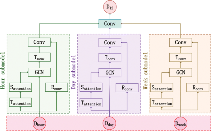
The framework of ASTGCN. Dhour: Recent training data; Dday: Daily-periodic training data; Dweek: Weekly-periodic training data; D12: The forecasted values of the next 12 time slots; Tattention: Temporal Attention; Sattention: Spatial Attention; GCN: Graph Convolution Network; Tconv: Temporal Convolution; Rconv: Residual Convolution; Conv: Common Standard Convolution
Sattention: A spatial attention mechanism, which can effectively capture the dynamic spatial correlation of traffic data.
GCN: A graph convolution network, which can capture spatial features of graph-based data.
Tconv: A temporal convolution, which can capture temporal dependencies from nearby time slices.
Rconv: A residual convolution, which can optimize the training efficiency of the model.
Conv: A common standard convolution, which can guarantee the dimension of the model output is the same as that of the forecasted target.

Specifically, given the current time t0, the size of forecasting window Tp, the historical data X of all nodes in the network over past τ time slices, the segment of historical time series directly adjacent to the predicting period serves as the input of the recent component (denoted as Dhour). Similarly, the segments in the past few days which have the same day attributes and time intervals as the forecasting period serve as the input of the daily-period component (denoted as Dday). The segments in the last few weeks which have the same week attributes and time intervals as the forecasting period serve as the input of the weekly-period component (denoted as Dweek). Noting that the length of these three inputs (Dhour, Dday and Dweek) is integer multiples of Tp. The three independent components respectively extract recent, daily-periodic and weekly-periodic data features from input data, and send them to the final fully connected layer. The final fully connected layer fuses the outputs of the three components based on the weights learned from historical data to obtain the forecasted value (denoted as D12), where the weights reflect the influence degrees of the outputs of the three components on the forecasting value.

Adaptive sample rate adjustment
Before the system works, a routing tree is constructed, which is the basis for data gathering. The ASTGCN model is trained by using historical traffic data and model parameters are saved in the cloud to forecast future traffic data. The procedure about adaptive sample rate adjustment is presented by Algorithm 1.
(i) Data structures in the cloud and IoT nodes.
The parameters of the model and the historical data of IoT nodes are cached in the cloud. They are denoted as the following vector: D=〈para,hdt〉, where para represents parameters of the model and hdt represents historical data of IoT nodes. hdt is represented by the following vector: hdt=〈d(1),d(2),⋯,d(i),⋯,d(N)〉, where \(d^{(i)} = \left \langle d_{1}^{(i)}, d_{2}^{(i)}, \cdots, d_{j}^{(i)}, \cdots, d_{m}^{(i)} \right \rangle \) represents time-series data of the i-th IoT node and \(d_{j}^{(i)}\) represents sensory data of the IoT node at the j-th time slot, which is routed by the IoT node or computed in the cloud using the prediction model. Without loss of generally, we assumed that the cloud has unlimited resources to store historical data and model parameters. Note that every IoT node maintains a record in terms of the following vector: ED=〈dt,label〉, where dt represents sensory data at the current time slot, label represents the category of sensory data at the current time slot.
(ii) Edge nodes compressing and routing data to the cloud.
As presented in Algorithm 1, for each IoT node, sensory data are encoded into binary category data through the strategy (as presented in “Sensory data classification and representation” section), which are routed to its corresponding edge node through a routing tree, when sensory data are sampled at the current time slot (line 1-4). For each edge network, category data are compressed in the edge node by using the CS algorithm (as presented in “Data compression in edge nodes” section) and are routed to the cloud later through the shortest path. In order to ensure the validity of the CS algorithm, whether data are compressed or not is determined by the sparsity of the data. If the sparsity of the data satisfies a certain condition, the data are compressed and routed to the cloud. Otherwise, the data are directly routed to the cloud through a routing tree (line 5-15).
(iii) Adaptive sample rate adjustment.
In the cloud, sensory data at the current time slot are forecasted by using the pre-trained ASTGCN model (as presented in “Data prediction model in the cloud” section) based on historical data. In order to detect whether the category of forecasted values in the cloud is consistent with that of actual ones of sensory data, the category of sensory data needs to be routed to the cloud from edge networks. Note that forecasted values in the cloud are encoded to category data by using the same strategy as IoT nodes of edge networks (line 16-19). If the category of a forecasted value is different from the category of actual one of sensory data, the forecasted value can’t be adopted instead of the actual one. At this time, the cloud notifies the IoT node to route sensory data at the current time slot and updates historical data by using the actual one. Otherwise, historical data are updated by using the forecasted value (line 20-26).
(iv) Calculate energy consumption.
Our energy consumption is calculated by using the energy model in “Energy model” section, which is mainly used for transmitting and receiving data in the following three processes:
Smart things send a k bits packet to edge nodes and edge nodes receive the k bits packet.
Edge nodes send a k bits packet to one-hop neighbor nodes and one-hop neighbor nodes receive the k bits packet.
IoT nodes send a k bits packet to the cloud but the cloud receiving the packet is ignored.
The operation presented in Algorithm 1 shows that the collaboration between the cloud and IoT nodes can reduce the volume of data that are routed in the networks. Thereby, it reduces the energy consumed by data transmission and extends the lifetime of the network. When a forecasted value meets the requirements of certain applications, sensory data don’t need to be routed to the cloud. This strategy can reduce the volume of sensory data to be routed in the network to a large extent, especially when the accuracy of the prediction model is greatly high in the cloud.
Implementation and evaluation
The prototype is implemented in the Python programing language on a laptop with an Intel(R) Core(TM) i7-7700 CPU at 2.80 GHz, 16 GB memory, and 64-bit Windows operating system. We evaluate our technique on the real highway traffic dataset PeMSD4 from California, which is available in (https://doi.org/https://github.com/wanhuaiyu/ASTGCN/tree/master/data/PEMS04). The dataset is collected by the Caltrans Performance Measurement System (PeMS), and 307 IoT nodes are deployed in the network. IoT nodes gather sensory data in real time with an interval as five minutes from January to February 2018, where each IoT node provides a total of 16,992 sensory data [20].
Environmental settings
An IoT network with 307 IoT nodes and one cloud is distributed in a geographical area of 100m ×100m, where IoT nodes are deployed evenly or unevenly with a skewness degree (e.g. 0%, 10%, 20%) and the cloud is located in the center (50m, 50m) or boundary (100m, 50m) of the area.
Once an IoT network is deployed, an appropriate radio transmission range is chosen according to IoT nodes’ density to make sure that the network is connected. Generally, IoT nodes can be connected to their neighbors within its radio transmission range. The communication radius is set to 35m, and the number of clusters is set to 1, 25, 64 in this paper. Note that the number of clusters is 1, which means that there is no area division in the IoT network. In the CS algorithm, the number of measurements is calculated according to the following formula: Mmin=1.1∗k∗ log(3N/k+1.7)+10, where N refers to the number of IoT nodes and k refers to the data’s sparsity. Note that the length of category data in [12] is larger than that in this paper. Therefore, the value of Mmin is larger and the accuracy of data recovery is also higher. The parameter settings used in this experiment are shown in Table 3.
Factors affecting performance evaluation
The following factors should be considered to evaluate the performance and efficiency of our technique.
1) Different data prediction models in the cloud. Intuitively, the higher the accuracy of data prediction models in the cloud is, the smaller the difference between the predicted value and sensory value is and thus the greater the probability that sensory values and prediction values fall into the same data interval is. In this paper, the consistency rate of data means the probability that sensory values and prediction values fall into the same data interval. Therefore, as the accuracy of data prediction models increases, the consistency rate of the data is increasing and the number of sensory data routed to the cloud is decreasing. In order to investigate the impact of different data prediction models on our technique, five data prediction models, namely HA, ARIMA, LSTM, GRU, and ASTGCN, are respectively adopted in our experiments for forecasting future sensory data of IoT nodes.
2) Whether or not the CCS mechanism is applied to the category data compression in edge nodes. Generally, there are the spatial-temporal correlations between sensory data, whose category data are sparse in the time domain. The CS algorithm can compress sparse category data, which reduces the volume of category data routed to the cloud and thus reduces the energy consumption of the network to an extent.
3) The different number of clusters in the network. Intuitively, the number of clusters affects the distance between smart things and edge nodes, the distance and the number of data transferred between edge nodes and the cloud. In order to study the impact of the number of clusters on our technique, the number of clusters is set to 1, 25, 64, respectively.
4) Various skewness degree of the distribution of IoT nodes. The distribution of IoT nodes affects the distance of data transmission of IoT nodes, and thus, affects the total energy consumption of the network. In order to study the impact of the distribution of IoT nodes on our technique, the skewness degree is set to 0%, 10%, 20%, respectively.
5) Different locations of the cloud. Intuitively, the location of the cloud affects the distance between edge nodes and the cloud. In order to study the impact of the location of the cloud on our technique, the cloud is located in (50m, 50m) and (100m, 50m), respectively.
Figure 3 represents the comparison of energy consumption when data prediction models are HA, ARIMA, LSTM, GRU, and ASTGCN in the cloud; IoT nodes are evenly and randomly deployed in the network; the cloud is located in the center of the area (50m, 50m). As shown in Fig. 3, the energy consumption is decreased when the data prediction model is changed from classical statistical models (ARIMA and HR) to machine learning models (LSTM and GRU) and the energy consumption is the lowest when the data prediction model is the ASTGCN model in the cloud. This is due to the fact that machine learning models (LSTM and GRU) can extract more useful information from historical data than classic statistical models (ARIMA and HR), and they have better prediction accuracy than classical statistical models. However, since they don’t consider the spatial correlation of sensory data, their prediction accuracy is not as good as that of the ASTGCN model. As shown in Fig. 4, the Root Mean Square Error (RMSE) of machine learning models is smaller than that of classical statistical models and the RMSE of the ASTGCN model is the smallest. Intuitively, the smaller the RMSE of the data prediction model is, the higher its accuracy is and the higher the consistency rate of data between the cloud and edge networks is. As shown in Fig. 5, ASTGGN model outperforms other techniques with the highest consistency rate in the cloud. Therefore, when the ASTGCN model is adopted to forecast data in the cloud, the number of sensory data transmitted is the least in the network. In other words, the model is the most energy-efficient.

Impact of different data prediction models in the cloud on energy consumption

RMSE of HA, ARIMA, LSTM, GRU and ASTGCN models

Consistency rate of data between the cloud and IoT nodes for different data prediction models
Figure 6 represents the comparison of energy consumption, where the nodes distribution skewness is set to 0%, 10%, and 20%, and the number of clusters is set to 1, 25 and 64. The energy consumption is reduced to a large extent when the number of clusters changes from 1 to 25. However, in contrast, the energy consumption is increased to a small extent when the number of clusters varies from 25 to 64. In fact, when the number of clusters ranges from 1 to 25, the data routed by edge nodes to the cloud change from category data to compressed data. Therefore, the volume of data transmission is greatly reduced, and the energy consumption of the network is significantly reduced. However, when the number of clusters ranges from 25 to 64, the number of clusters is the main influencing factor of energy consumption. Specifically, as the number of clusters increases, the energy is lightly decreased that is consumed by data transmission between smart things and edge nodes, while the energy is obviously increased that is consumed by routing data between edge nodes and the cloud. This leads to an increase in total energy consumption.

The effect of skewness and the number of clusters on energy consumption when the cloud is located in the center of the area (50m, 50m). NoC represents the number of clusters in the IoT network
Besides, Fig. 6 shows, as the number of clusters changes, the changing trend of energy consumption is similar when the skewness is 0%, 10%, and 20%. This means that our mechanism is not only suitable for evenly distributed networks but also unevenly distributed networks. In other words, it can reduce energy consumption in networks of different skewness.
Figures 6 and 7 present the energy consumption when the cloud is located in the center and boundary of the IoT area respectively. The energy consumption of Fig. 7 is much higher than that of Fig. 6 with the same skewness and number of clusters. It implies that the location of the cloud has a great impact on the total energy consumption. When the cloud is located in the boundary of the IoT area, most edge nodes are farther away from the cloud. This leads to more energy consumed by data transmission from edge nodes to the cloud and an increase in the total energy consumption.

The effect of skewness and the number of clusters on energy consumption when the cloud is located in the region-al boundary (100m, 50m). NoC represents the number of clusters in the IoT network
Comparison of energy consumption with DBP
This section compares the energy consumption of our technique (denoted as CCS &ASTGCN) with that of the Derivative-based Prediction mechanism (denoted as DBP). For the DBP mechanism, the DBP data prediction model is deployed simultaneously in the cloud and IoT nodes. IoT nodes decide whether to route sensory data to the cloud by checking whether forecasted values meet the requirements of certain applications. Only when forecasted values don’t meet the requirements of certain applications, are the model parameters and sensory data routed to the cloud to ensure the synchronization between the cloud and IoT nodes in terms of the prediction model and sensory data. Otherwise, it’s not necessary for IoT nodes to route sensory data and model parameters to the cloud.
Figure 8 illustrates the energy consumption of DBP and CCS &ASTGCN strategy when the skewness of nodes distribution is set to 0%, 10%, 20%; the cloud is located in the center (50m, 50m) and boundary (100m, 50m) of the IoT area; the number of clusters is set to 25. The results show that our mechanism consumes less energy than the DBP strategy with the same skewness of IoT nodes and location of the cloud. Its main reason is not the reduction of sensory data to be routed to the cloud, but the fact that the model parameters don’t need to be routed to the cloud in our mechanism. As shown by the experimental result, the accuracy of the DBP data prediction model is similar to that of the ASTGCN data prediction model, which leads to the same number of sensory data to be routed to the cloud for the two strategies. However, the ASTGCN model, as a neural network model, doesn’t need to be updated in real time. In other words, the ASTGCN model parameters don’t need to be routed to the cloud when forecasted values don’t meet the requirements of certain applications.

Comparison of energy consumption of DBP and CCS&ASTGCN mechanism with various skewness of nodes distribution and locations of the cloud
Comparison of energy consumption with PCA
This section compares the energy consumption of the Principal Component Analysis strategy (denoted as PCA) with that of our technique CCS &ASTGCN. For the PCA strategy, sensory data are compressed in edge nodes by using the PCA algorithm. Edge nodes determine the dimension of compressed data by checking whether decompressed data meet the requirements of a certain application. This strategy can reduce the transmission of redundant data in the IoT network while meeting the requirements of a certain application.
Figure 9 illustrates the energy consumption of PCA and CCS &ASTGCN strategy when the skewness of IoT nodes distribution is set to 0%, 10%, and 20%; the cloud is located in the center (50m, 50m) and boundary (100m, 50m) of the IoT area; the number of clusters is set to 25. The results show that our mechanism consumes less energy than the PCA strategy with the same skewness of IoT nodes and location of the cloud. Its main reason is as follows: for the PCA strategy, edge nodes route compressed sensory data to the cloud all the time. However, in our strategy, edge nodes upload compressed category data to the cloud all the time, and sensory data are routed to the cloud only when forecasted values in the cloud don’t meet the requirements of a certain application. Here, sensory data don’t need to be routed to the cloud at most time slots, since the accuracy of the prediction model in the cloud is very high in our strategy. This greatly reduces the transmission of sensory data in the network. However, compared to the PCA strategy, category data are additional data in our strategy. Generally, their bits are much smaller than that of sensory data, which means that they have a much smaller volume than sensory data. Therefore, the energy consumed by the transmission of category data is much less than the energy saved by the reduction of the transmission of sensory data. This makes our strategy more energy efficient than the PCA strategy.

Comparison of energy consumption of PCA and CCS&ASTGCN mechanism with various skewness of nodes distribution and locations of the cloud
Related work
Energy-Efficient mechanism for data gathering
The IoT technology has been widely applied in various domains for continuously monitoring environmental variables. In the process, IoT nodes periodically sense, collect and forward data, which leads to an increase in their energy consumption [21]. Besides, they are typically powered by batteries, and it is often difficult for them to be recharged and replaced after the initial deployment. Hence, energy efficiency is of great importance to support continuous data gathering.
There are many ways to gather sensory data in an energy-efficient way. The combination of the CS algorithm and routing techniques is a mainstream way of energy-saving data gathering. Here, routing techniques are divided into the cluster-based, tree-based, random walk routing technique and so on. In densely deployed networks, as shown in our paper, the CCS algorithm [13] is adopted to collect category data in edge networks, which significantly reduces the energy consumption of data transmission in IoT networks. In [10], Luo et al. proposed the first complete Compressive Data Gathering (CDG) method in large-scale WSN. However, the volume of compressed data is increased in the condition that the number of sensory data is smaller than the number of measurements M. In order to optimize the algorithm, Xiang et al. [11] put forward a data aggregation technique called Hybrid-CS. Here, sensory data are compressed by the CS algorithm, only when the number of sensory data exceeds M. Otherwise, sensory data are directly routed to parents’ nodes. However, this algorithm doesn’t realize the function of the real-time adjustment of the number of measurements based on the extent of sensory data sparseness. In [12], the authors developed an MST-MA-GSP algorithm, which can solve this problem to make sure the value of M as small as possible while maximizing data reconstruction performance. This algorithm can balance the energy consumption among sensor nodes. However, it can’t minimize the total energy consumption of IoT networks.
In [22], Mamaghanian et al. compared three kinds of random sensing matrices, such as quantized Gaussian random sensing matric, pseudo-random sensing matric, and sparse binary sensing matric. The CS algorithm is superior in terms of execution time when a sparse binary sensing matrix is adopted as the measurement matrix. By utilizing the matrix, Li and Qi [23] proposed a Distributed Compressive Sparse Sampling (DCSS) algorithm, where M encoding nodes are selected for sampling data and compressed data are routed to a Fusion Center (FC) by the shortest path.
In [24], the authors proposed a data aggregation algorithm based on the PCA, where sensory data are compressed by utilizing the PCA algorithm in edge nodes, and routed to the cloud later. Therefore, it greatly reduces the volume of sensory data in the networks. However, edge nodes need to collect data at multiple time slots from smart things, and then compress and send these data to the cloud, which causes that the cloud can’t get sensory data in real time.
In [25, 26], the authors proposed an adaptive sampling strategy to reduce the number of data sampling, where sensory data are routed to the sink node only when a significant change is detected by sensor nodes. But, in the strategy, the determination of the threshold is challenging and it needs to be set according to the experience of people. Gabriel et al. [27] proposed a dynamic sampling rate adaptation scheme based on reinforcement learning algorithm, where the sampling rate is dynamically adjusted based on the analysis of historical data in real time, which eliminates the errors caused by the subjective factors of people outside the system. Note that the data in the cloud can’t be dynamically updated over time during some time intervals in this strategy. In [14, 15], a simple linear function, named DBP method, is simultaneously adopted in the cloud and IoT nodes to forecast sensory data. Only when forecasted values don’t meet the requirements of certain applications, this is, the difference between the values of sensory data being forecasted and being sensed in real time exceeds a preset value, sensory data and model parameters of sensor nodes are routed to the cloud to synchronize with the cloud. Otherwise, it isn’t necessary to route sensory data to the cloud. This strategy greatly reduces the amount of data transmission and the energy consumption of IoT networks while updating data in the cloud over time in real time, especially when the variation trend of data is simple and predictable. However, once the data change dramatically, the performance of the strategy will be greatly reduced.
The sleep/wake-up scheduling strategy is commonly used for gathering data in WSN. It can reduce the energy consumption of the network by minimizing idle listening time and reducing the number of state switching of sensor nodes. In [3], based on the characteristics of the minimum hop routing, the authors designed two different strategies for terminal nodes and intermediate nodes to make sensor nodes periodically sleep and wake up. This method can reduce idle listening time to prolong the network lifetime. However, the energy is nonnegligible that is consumed by state transitions. To further reduce the energy consumption of the network, Yanwei Wu et al. [28] proposed a data gathering strategy to minimize wake-up time, where every sensor node only waken up at most twice a scheduling period. However, this method can’t achieve optimal energy consumption and data delivery time delay at the same time. In [29], the authors proposed a radio-triggered wake-up scheme, which can wake up sensor nodes by utilizing the radio loop to trigger an interrupt. Moreover, this technology has lower time latency and less energy consumption than the rotation-based wake-up strategy. However, some interferences between data transmission and wake up have not been alleviated. The work [30] solves this problem by utilizing a special frequency band that is different from the data transmission frequency band.
Since the sleep/wake-up scheduling strategy can’t solve the hot spot problem, the data gathering algorithm based on mobile sinks can successfully alleviate it by using mobile devices outside the system, which can be used in connected and unconnected networks. To prolong the network lifetime, authors in [5, 31] proposed the tour planning strategy based on a mobile sink that can achieve energy efficiency and balance the load of the network. However, this method increases data delivery time delay and data loss due to the failure of (or infrequently) visiting some fields. To decrease the time delay, authors in [4], proposed a new data gathering mechanism by utilizing multiple mobile sinks. This method can improve energy efficiency and decrease the time delay by the cooperation between multiple mobile sinks, no matter when the network is a small-scale or large-scale network. However, since the path and trajectory are pre-existing in real applications, the optimal trajectory under ideal conditions sometimes can’t be realized, which leads to increases in energy consumption, delivery delay, and even packet loss rate. For continuous monitoring applications, this method is not applicable under strict time constraints and its tight cost.
Algorithms for data prediction
Data prediction models have gone through three special stages: classical statistical models, machine learning models, and deep learning models. Besides, data prediction models are generally classified into short-term and long-term data prediction models. The most universal statistical methods are able to perform well for simple and short-term prediction. However, they perform poorly for the complex and long-term spatial-temporal data prediction.
In IoT networks, it is usually more simple and convenient to collect and store data. Data-driven data prediction methods are used for forecasting data and able to perform well on complex data prediction, in which classical statistical models and machine learning models are two kinds of representative models [32]. In time series analysis, AutoRegressive Integrated Moving Average (ARIMA) and its variants are one of the most consolidated classical statistics approaches [33]. Note that these models are limited by the stationary assumption of time sequences and fail to take into account the spatial correlation. Therefore, their accuracy is often not satisfying for the highly nonlinear spatial-temporal data prediction. However, machine learning methods (such as k-nearest neighbors algorithm [34], tree regression [35], neural networks models [36], etc.), as more complex models, can extract more useful information from historical data [37], and thus, their accuracy is higher than that of classical statistical models.
Compared with machine learning models, deep learning models have higher accuracy by utilizing the spatial-temporal correlations of data. Wu and Tan [38] proposed a novel deep learning architecture to forecast future traffic flows, where a one-dimension CNN is adopted to capture spatial features of traffic data and two LSTMs are utilized to get the short-term variability and periodicity of traffic data, which is the first attempt to forecast traffic data by considering the spatial-temporal correlations of data. However, the normal convolutional operation limits that data to be processed must be grid data. Yu and Yin [32] proposed a novel deep learning framework, named Spatio-Temporal Graph Convolutional Networks (STGCN), to solve time series prediction problems in the field of transportation. It directly implements convolution operations on graph-structured data to effectively capture comprehensive spatial-temporal correlations of the data, which could greatly improve prediction accuracy. But it doesn’t consider the inherent characteristics of the periodicity of traffic data in the time dimension. Yu and Yin [20] proposed a novel ASTGCN model, which can simultaneously capture the dynamic spatial-temporal correlations, the spatial patterns, and the temporal features, and thus, it has high prediction accuracy on the long-term spatial-temporal data prediction. Therefore, in this paper, it is used as a data prediction model in the cloud.
Conclusion
This paper proposes an energy-efficient sensory data gathering mechanism. Specifically, sensory data are encoded into binary category data in IoT nodes, and then they are routed to their corresponding edge nodes through a routing tree. For each edge network, category data are compressed using the CS algorithm in its edge node and routed to the cloud through the shortest path later. In the cloud, sensory data are forecasted by using an accurate data prediction model. Only when the category of forecasted values is different significantly from that of sensory values, dose the cloud notify IoT nodes to route their sensory data. Leveraging this mechanism, sensory data are continuously gathered to support environmental monitoring. Experimental evaluation shows that this technique can reduce the energy consumption of IoT networks to an extent without lowering the satisfiability of certain requirements, especially when network environments changes frequently and strong spatial-temporal correlations exist between sensory data.
Availability of data and materials
The data is available in (https://doi.org/https://github.com/wanhuaiyu/ASTGCN/tree/master/data/PEMS04).
Abbreviations
- IoT:
-
Internet of things
- ITS:
-
Intelligent transportation systems
- WSN:
-
Wireless sensor networks
- CS:
-
Compressed sensing
- CCS:
-
Cluster-based compressive sensing
- ASTGCN:
-
Attention-based spatial-temporal graph convolutional network
- BP:
-
Basis pursuit
- PeMS:
-
Caltrans performance measurement system
- DBP:
-
Derivative-based prediction
- PCA:
-
Principal component analysis
- CDG:
-
Compressive data gathering
- DCSS:
-
Distributed compressive sparse sampling
- FC:
-
Fusion center
- ARIMA:
-
AutoRegressive integrated moving average
- STGCN:
-
Spatio-temporal graph convolutional networks
References
Veres M, Moussa M (2019) Deep learning for intelligent transportation systems: A survey of emerging trends. IEEE Trans Intell Transp Syst. https://doi.org/10.1109/TITS.2019.2929020.
Monil MAH, Rahman RM (2016) VM consolidation approach based on heuristics, fuzzy logic, and migration control. J Cloud Comput. https://doi.org/10.1186/s13677-016-0059-7.
Ren Z, Shi S, Wang Q, Yao Y (2011) A node sleeping algorithm for wsns based on the minimum hop routing protocol. Int Conf Comput Manag. https://doi.org/10.1109/CAMAN.2011.5778776.
Zhang J, Tang J, Wang T, Chen F (2017) Energy-efficient data-gathering rendezvous algorithms with mobile sinks for wireless sensor networks. Int J Sensor Netw 23:248–257.
Huang H, Savkin AV (2017) An energy efficient approach for data collection in wireless sensor networks using public transportation vehicles. AEU Int J Electron Commun 75:108–118.
Kaswan A, Nitesh K, Jana PK (2017) Energy efficient path selection for mobile sink and data gathering in wireless sensor networks. AEU Int J Electron Commun 73:110–118.
Giridhar A, Kumar PR (2017) Computing and communicating functions over sensor networks. IEEE J Sel Areas Commun 23:755–764.
Zhang Y, Cui G, Deng S, Chen F, Wang Y, He Q (2018) Efficient Query of Quality Correlation for Service Composition. IEEE Trans Serv Comput. https://doi.org/10.1109/TSC.2018.2830773.
Khan S, Parkinson S, Qin Y (2017) Fog computing security: a review of current applications and security solutions. J Cloud Comput. https://doi.org/10.1186/s13677-017-0090-3.
Luo C, Wu F, Sun J, Chen CW (2009) Compressive data gathering for large-scale wireless sensor networks In: Proceedings of the 15th annual international conference on Mobile computing and networking. https://doi.org/10.1145/1614320.1614337.
Xiang L, Luo J, Rosenberg C (2013) Compressed data aggregation: Energy-efficient and high-fidelity data collection. IEEE/ACM Trans Netw 21:1722–1735.
Lv C, Wang Q, Yan W, Li J (2018) A sparsity feedback-based data gathering algorithm for Wireless Sensor Networks. Comput Netw 141:145–156.
Nguyen MT, Teague KA, Rahnavard N (2016) CCS: Energy-efficient data collection in clustered wireless sensor networks utilizing block-wise compressive sensing. Comput Netw 106:171–185.
Raza U, Camerra A, Murphy AL, Palpanas T, Picco GP (2015) Practical data prediction for real-world wireless sensor networks. IEEE Trans Knowl Data Eng 27(8):2231–2244.
Zhou Z, Fang W, Niu J, Shu L, Mukherjee M (2017) Energy-efficient event determination in underwater WSNs leveraging practical data prediction. IEEE Trans Ind Inform 13(3):1238–1248.
Wu M, Tan L, Xiong N (2016) Data prediction, compression, and recovery in clustered wireless sensor networks for environmental monitoring applications. Inform Sci 329:800–818.
Zhou Z, Zhao D, Hancke G, Shu L, Sun Y (2016) Cache-aware query optimization in multiapplication sharing wireless sensor networks. IEEE Trans Syst Man Cybernet Syst 48:401–417.
Li X, Zhou Z, Guo J, Wang S, Zhang J (2019) Aggregated multi-attribute query processing in edge computing for industrial IoT applications. Comput Netw 151:114–123.
Ping H, Zhou Z, Shi Z, Rahman T (2018) Accurate and energy-efficient boundary detection of continuous objects in duty-cycled wireless sensor networks. Pers Ubiquit Comput 22:597–613.
Guo S, Lin Y, Feng N, Song C, Wan H (2019) Attention Based Spatial-Temporal Graph Convolutional Networks for Traffic Flow Forecasting. Proc 33rd AAAI Conf Artif Intell 33:992–929.
Xu X, Liu Q, Zhang X, Zhang J, Qi L, Dou W (2019) A Blockchain-Powered Crowdsourcing Method With Privacy Preservation in Mobile Environment. IEEE Trans Comput Soc Syst 6(6):1407–1419.
Mamaghanian H, Khaled N, Atienza D, Vandergheynst P (2011) Compressed sensing for real-time energy-efficient ECG compression on wireless body sensor nodes. IEEE Trans Biomed Eng 58(9):2456–2466.
Li S, Qi H (2013) Distributed data aggregation for sparse recovery in wireless sensor networks In: IEEE International Conference on Distributed Computing in Sensor Systems, 62–69. https://doi.org/10.1109/dcoss.2013.64.
Li J, Guo S, Yang Y, He J (2016) Data aggregation with principal component analysis in big data wireless sensor networks In: 12th International Conference on Mobile Ad-Hoc and Sensor Networks, 45–51. https://doi.org/10.1109/msn.2016.015.
Endo PT, Rodrigues M, Goncalves GE, Kelner J, Sadok DH, Curescu C (2016) High availability in clouds: systematic review and research challenges. J Cloud Comput. https://doi.org/10.1186/s13677-016-0066-8.
Al-Hoqani N, Yang S-H (2015) Adaptive sampling for wireless household water consumption monitoring. Procedia Eng 119:1356–1365.
Dias GM, Nurchis M, Bellalta B (2016) Adapting sampling interval of sensor networks using on-line reinforcement learning In: IEEE 3rd World Forum on Internet of Things, 460–465. https://doi.org/10.1109/wf-iot.2016.7845391.
Wu Y, Li X-Y, Li Y, Lou W (2009) Energy-efficient wake-up scheduling for data collection and aggregation. IEEE Trans Parallel Distrib Syst 21:275–287.
Gu L, Stankovic JA (2005) Radio-triggered wake-up for wireless sensor networks. Real-Time Syst 29:157–182.
Miller MJ, Vaidya NH (2004) Power save mechanisms for multi-hop wireless networks In: First International Conference on Broadband Networks, 518–526. https://doi.org/10.1109/broadnets.2004.67.
Zhu C, Wu S, Han G, Shu L, Wu H (2015) A tree-cluster-based data-gathering algorithm for industrial WSNs with a mobile sink. IEEE Access 3:381–396.
Yu B, Yin H, Zhu Z (2017) Spatio-temporal graph convolutional networks: A deep learning framework for traffic forecasting In: Proceedings of the 27th International Joint Conference on Artificial Intelligence, 3634–3640. https://doi.org/10.24963/ijcai.2018/505.
Eymen A, Köylü Ü (2019) Seasonal trend analysis and ARIMA modeling of relative humidity and wind speed time series around Yamula Dam. Meteorol Atmospheric Phys 131:601–612.
Martínez F, Frías MP, Pérez MD, Rivera AJ (2019) A methodology for applying k-nearest neighbor to time series forecasting. Artif Intell Rev 52:11–17.
Xu Y, Kong Q-J, Liu Y (2013) Short-term traffic volume prediction using classification and regression trees. IEEE Intell Veh Symposium:493–498. https://doi.org/10.1109/ivs.2013.6629516.
Zhang Y, Yin C, Wu Q, He Q, Zhu H (2019) Location-Aware Deep Collaborative Filtering for Service Recommendation. IEEE Trans Syst Man Cybernet Syst. https://doi.org/10.1109/TSMC.2019.2931723.
Qi L, He Q, Chen F, Dou W, Wan S, Zhang X, Xu X (2019) Finding All You Need: Web APIs Recommendation in Web of Things Through Keywords Search. IEEE Trans Comput Soc Syst 6(5):1063–1072.
Wu Y, Tan H (2016) Short-term traffic flow forecasting with spatial-temporal correlation in a hybrid deep learning framework:1–14. arXiv:1612.01022.
Acknowledgments
The authors thank the editor and anonymous reviewers for their helpful comments and valuable suggestions. I would like to acknowledge all our team members.
Funding
This work was supported by the National Natural Science Foundation of China (Grant no. 61772479 and 61662021).
Author information
Authors and Affiliations
Contributions
Authors’ contributions
The research work is a part of Xinxin Du master’s work, which is being conducted under the supervision and guidance of Zhangbing Zhou professor. All authors take part in the discussion of the work described in this paper. All authors read and approved the final manuscript.
Authors’ information
Xinxin Du is a master student at School of Information Engineering, China University of Geosciences (Beijing). Her research interests include edge computing and IoT networks. Email:xinxindu@cugb.edu.cn.
Zhangbing Zhou is a professor at School of Information Engineering, China University of Geosciences (Beijing), China, and an adjunct professor at TELECOM SudParis, Evry, France. His research interests include wireless sensor networks, services computing and business process management. Email: zbzhou@cugb.edu.cn. Corresponding author.
Yuqing Zhang is a associate professor at China University of Geosciences (Beijing), China. His research interests include services computing and wireless sensor networks. Email: yqzhang@cugb.edu.cn.
Taj Rahman is an assistant professor at the department of computer science and IT, Qurtuba University of Science and Technology Peshawar, Pakistan. He received the B.S degree in computer science from University of Malakand Dir (lower) Pakistan, in 2007 and the M.S degree in computer science from Agriculture University Peshawar Pakistan, in 2011. He received his Ph.D degree in computer science from the school of computer and communication engineering, University of Science and Technology Beijing, China. His research interests include Wireless Sensor Networks, Internet of Things and edge computing. Email: tajuom@gmail.com or softrays85@yahoo.com.
Corresponding author
Ethics declarations
Competing interests
The authors declare that they have no competing interests. They have seen the manuscript and approved to submit to your journal. We confirm that the content of the manuscript has not been published or submitted for publication elsewhere.
Additional information
Publisher’s Note
Springer Nature remains neutral with regard to jurisdictional claims in published maps and institutional affiliations.
Rights and permissions
Open Access This article is licensed under a Creative Commons Attribution 4.0 International License, which permits use, sharing, adaptation, distribution and reproduction in any medium or format, as long as you give appropriate credit to the original author(s) and the source, provide a link to the Creative Commons licence, and indicate if changes were made. The images or other third party material in this article are included in the article’s Creative Commons licence, unless indicated otherwise in a credit line to the material. If material is not included in the article’s Creative Commons licence and your intended use is not permitted by statutory regulation or exceeds the permitted use, you will need to obtain permission directly from the copyright holder. To view a copy of this licence, visit http://creativecommons.org/licenses/by/4.0/.
About this article

Cite this article
Du, X., Zhou, Z., Zhang, Y. et al. Energy-efficient sensory data gathering based on compressed sensing in IoT networks. J Cloud Comp 9, 19 (2020). https://doi.org/10.1186/s13677-020-00166-x
Received:
Accepted:
Published:
DOI: https://doi.org/10.1186/s13677-020-00166-x