Stability analysis for a time-delayed nonlinear predator–prey model

Abstract

In this paper, we investigate the dynamics of a time-delayed prey–predator system with θ-logistic growth. Our investigation indicates that the models based on delayed differential equations (DDEs) with and without delay-dependent coefficient both undergo Hopf bifurcation at their corresponding positive equilibria. It is shown that stability switching occurs for the interior equilibrium of the model with delay-dependent coefficient. For the DDEs model without delay-dependent coefficient, increased time delay may destabilize a stable interior equilibrium.

1 Introduction

In biomathematics, the interaction and interplay between different species have been modeled by systems of differential equations. Such systems characterize the dynamics of a variety of ecosystems. By constructing an ecological model, the relationship between different species in the system is revealed. Analyzing such models yields the dynamics of the system and may give a precise prediction on the evolution of populations in the system. Recently, prey refuge has been integrated into ecological models to consider the effects of the refuges on the coexistence of different species and on the stability of equilibria of ecosystems [1–6]. Empirical and theoretical studies have both been carried out to illustrate the influences of prey refuge on the population dynamics of the systems. Investigations indicate that the existence of prey refuge may stabilize the system and by using such refuge, the prey population may refrain from extinction [7–13].

Tsoularis and Wallace [14] performed a thorough study on a variety of growth equations to model population dynamics and presented a generalized form of the logistic growth equation. Wonlyul and Kimun [15] analyzed a general Gause-type predator–prey model and investigated the existence and non-existence of non-constant positive steady-state solutions. Motivated by the works of Tsoularis and Wallace [14], and Wonlyul and Kimun [15], we construct the following θ-logistic growth predator–prey system with prey refuge:

$$ \begin{aligned} &\dot{x}=rx\biggl[1-\biggl(\frac{x}{K} \biggr)^{\theta}\biggr]-\frac{\beta \varepsilon^{2} x^{2}y}{1+\varepsilon^{2} x^{2}}-h_{1}x, \\ &\dot{y}=\frac{\beta\varepsilon^{2} x^{2}y}{1+\varepsilon^{2} x^{2}}-ay-h_{2}y. \end{aligned} $$

(1.1)

In system (1.1), the predator’s fitness increases with the consumption of prey. If we assume that for the predator species there is a time lag between the consumption of prey and the increase of predators’ fitness, then time delay should be integrated into the model. The ecological model incorporating such time delay is given by

$$ \begin{aligned} &\dot{x}=rx\biggl[1-\biggl(\frac{x}{K} \biggr)^{\theta}\biggr]-\frac{\beta \varepsilon^{2} x^{2}y}{1+\varepsilon^{2} x^{2}}-h_{1}x, \\ &\dot{y}=\frac{ e^{-m\tau}\beta\varepsilon^{2} x(t-\tau)^{2}y(t-\tau)}{1+\varepsilon^{2} x(t-\tau)^{2}}-ay-h_{2}y, \end{aligned} $$

(1.2)

where x and y respectively denote the densities of prey and predator, and r, K, θ, β, ε, a, and m take positive values. In system (1.2), the prey species has θ-logistic growth with logistic index θ and intrinsic growth rate r. Here, K is the carrying capacity, β is the predation rate of predator, and $\varepsilon\in(0, 1)$ is the refuge rate to prey. Obviously, $1-\varepsilon$ is the proportion of prey that is available for the predator. We use $h_{1}$ and $h_{2}$ to denote the rate of harvesting or the environment feedback for prey and predator, respectively. We assume that the predator has death rate a. The time lag between the consumption of prey and receiving corresponding increase in predator population is denoted by τ. We thus introduce a delay-dependent coefficient $e^{-m\tau}$ to describe the probability of the predators that consume prey at time $t-\tau$ and still remain alive at time t. Such delay-dependent coefficient may have considerable influences on the dynamical behaviors of the model and it has not been investigated extensively in the literature. In the following, we compare the dynamical behaviors of the model with and without the delay-dependent coefficient.

System (1.2) has the initial conditions

$$ \begin{aligned} &x(\eta)=\phi(\eta)\geq0,\qquad y(\eta)=\psi(\eta)\geq0, \quad \eta\in[-\tau, 0], \\ &\phi(0)>0,\qquad \psi(0)>0, \end{aligned} $$

(1.3)

where $(\phi(\eta), \psi(\eta))\in C([-\tau, 0], R^{2}_{+0})$ is the Banach space of continuous functions mapping the interval $[-\tau, 0]$ into $R^{2}_{+0}$, where $R^{2}_{+0}=\{(x, y): x\geq0, y\geq0\}$.

It follows from the fundamental theory of functional differential equations [16] that system (1.2) has a unique solution $x(t)$, $y(t)$ satisfying initial conditions (1.3).

This manuscript is organized as follows. In Sect. 2, we prove that solutions to system (1.2) with initial conditions (1.3) are positive and ultimately bounded. In Sect. 3, we investigate the stability of the boundary equilibria of system (1.2). In Sect. 4, we show that system (1.1) and (1.2) exhibits Hopf bifurcations at the interior equilibrium. Finally, we perform numerical analysis to illustrate the main results of this article in Sect. 5.

2 Positivity and boundedness

For model (1.2) with initial conditions (1.3), we are particularly interested in the positivity and boundedness of its solution. In this section, we prove that the solutions are positive and ultimately bounded.

2.1 Positivity of solutions

Theorem 2.1

Solutions to system (1.2) with initial conditions (1.3) are positive for all $t\geq0$.

Proof

Assume that $(x(t), y(t))$ is a solution to system (1.2) satisfying initial conditions (1.3). It follows from the first equation of model (1.2) that

$$x(t)=x(0)e^{\int_{0}^{t} \{r[1-(\frac{x(\zeta)}{K})^{\theta}]-\frac {\beta \varepsilon^{2} x(\zeta)y(\zeta)}{1+\varepsilon^{2} x(\zeta)^{2}} \}\,d\zeta}, $$

implying that $x(t)$ is positive.

Next we show that $y(t)$ is positive on $[0, +\infty)$. Assume that there exists $t_{1}$ such that $y(t_{1})=0$, and $y(t)>0$ for $t\in[0, t_{1})$. It thus follows that $\dot{y}(t_{1})\leq0$. Using the second equation of (1.2), we obtain

$$\begin{aligned} \dot{y}(t_{1}) =&\frac{ e^{-m\tau}\beta\varepsilon^{2} x(t-\tau)^{2}y(t_{1}-\tau)}{1+\varepsilon^{2} x(t_{1}-\tau )^{2}}-ay(t_{1})-h_{2}y(t_{1}) \\ =&\frac{ e^{-m\tau}\beta\varepsilon^{2} x(t-\tau)^{2}y(t_{1}-\tau)}{1+\varepsilon^{2} x(t_{1}-\tau)^{2}} \\ >&0. \end{aligned}$$

The above expression is a contradiction, which completes the proof of positivity. □

In the following subsection, we show that the solutions are ultimately bounded.

2.2 Boundedness of solutions

Theorem 2.2

Positive solutions of system (1.2) with initial conditions (1.3) are ultimately bounded.

Proof

Suppose that $(x(t), y(t))$ is a solution to system (1.2) and satisfies conditions (1.3). Then it follows from the first equation of (1.2) that

$$\dot{x}\leq rx \biggl[1-\biggl(\frac{x}{K}\biggr)^{\theta} \biggr]. $$

Thus, we have

$$x(t)\leq \frac{x_{0}K}{ [x_{0}^{\beta}+(K^{\beta}-x_{0}^{\beta})e^{-r\theta t} ]^{\frac{1}{\theta}}}. $$

That is to say,

$$\limsup_{t\rightarrow+\infty} x(t)\leq K. $$

It follows from the above discussion that, for sufficiently small ρ, there exists $T_{1}>0$ such that if $t>T_{1}$, $x(t)< K+\rho$. In order to prove the boundedness of the solution, we construct the following Lyapunov function:

$$V(t)=x(t-\tau)e^{-m\tau}+y(t). $$

Evaluating the derivative of V along the trajectories of system (1.2) yields

$$\begin{aligned} \begin{aligned} \dot{V}(t)&= e^{-m\tau}rx(t-\tau)\biggl[1-\biggl(\frac{x(t-\tau)}{K} \biggr)^{\theta }\biggr]-e^{-m\tau}h_{1}x(t-\tau) \\ &\quad {}-(a+h_{2})y(t) \\ &\leq e^{-m\tau}(r-h_{1})x(t-\tau)-(a+h_{2})y(t) \\ &\leq M_{0}-(a+h_{2})V(t), \end{aligned} \end{aligned}$$

where $M_{0}=e^{-m\tau}(r-h_{1})(K+\rho)$. It thus follows that there exists $M>0$ such that $V(t)\leq M$ for all t large enough. We notice that M only depends on the parameters of system (1.2). The above discussion implies that $x(t)$, $y(t)$ is ultimately bounded. □

3 Stability of the boundary equilibria

In the following, we consider the stability of the boundary equilibria of model (1.2) satisfying initial conditions (1.3).

Let $R_{0}=\frac{K\varepsilon(\frac{r-h_{1}}{r})^{\frac{1}{\theta}}\sqrt {(a+h_{2})(\beta e^{-m\tau}-a-h_{2})}}{a+h_{2}}$, and always assume that $r>h_{1}$ and $\beta>a+h_{2}$. Then system (1.2) has two boundary equilibria, given by $E_{0}=(0,0)$ and $E_{1}=(K(\frac{r-h_{1}}{r})^{\frac{1}{\theta}},0)$. If $R_{0}>1$, the system admits an interior (positive) equilibrium $E^{*}=(x^{*}, y^{*})$, where

$$\begin{aligned}& x^{*}=\frac{\sqrt{ (a+h_{2} ) (\beta e^{-m\tau}-a-h_{2} )}}{\varepsilon (\beta e^{-m\tau}-a-h_{2} )}, \\& y^{*}=\frac{ (1+\varepsilon^{2} x^{*2} ) [r-h_{1}-r(\frac{x^{*}}{K})^{\theta} ]}{\beta \varepsilon^{2}x^{*2}}. \end{aligned}$$

The characteristic equation of the model corresponding to $E_{0}=(0,0)$ is

$$(\lambda-r+h_{1}) (\lambda+a+h_{2})=0, $$

whose roots are obtained as

$$\lambda_{1}=r-h_{1}>0 \quad \mbox{and}\quad \lambda_{2}=-a-h_{2}< 0. $$

It thus follows that equilibrium $E_{0}$ is unstable.

The characteristic equation of the model with respect to $E_{1}=(K,0)$ is obtained as

$$\bigl[\lambda+\theta(r-h_{1}) \bigr] \biggl[\lambda+a+h_{2}- \frac{\beta e^{-m\tau}\varepsilon^{2}x_{1}^{2}e^{-\lambda\tau}}{1+\varepsilon ^{2}x_{1}^{2}} \biggr]=0, $$

implying that

$$\lambda_{1}=-\theta(r-h_{1}) $$

and

$$\lambda+a+h_{2}-\frac{\beta e^{-m\tau}\varepsilon ^{2}x_{1}^{2}e^{-\lambda\tau}}{1+\varepsilon^{2}x_{1}^{2}}=0. $$

Let

$$f(\lambda)=\lambda+a+h_{2}-\frac{\beta e^{-m\tau}\varepsilon ^{2}x_{1}^{2}e^{-\lambda\tau}}{1+\varepsilon^{2}x_{1}^{2}}. $$

Therefore,

$$\begin{aligned} f(0) =&a+h_{2}-\frac{\beta e^{-m\tau}\varepsilon ^{2}x_{1}^{2}}{1+\varepsilon^{2}x_{1}^{2}} \\ =& \frac{a+h_{2}}{1+\varepsilon^{2}x_{1}^{2}}\bigl(1-R_{0}^{2}\bigr) \end{aligned}$$

and

$$\lim_{\lambda\rightarrow\infty}f(\lambda)=\infty $$

for any $\tau\geq0$. Thus, if $R_{0}\leq1$, $f(\lambda)=0$ has no positive root. If $R_{0}>1$, $f(\lambda)=0$ has at least one positive root. It thus follows that, for all $\tau\geq0$, when $R_{0}\leq1$, equilibrium $E_{1}$ is stable. When $R_{0}>1$, the equilibrium is unstable.

The above results are summarized in the following conclusion.

Theorem 3.1

• (i) For all $\tau\geq0$, equilibrium $E_{0}$ is always unstable.

• (ii) For all $\tau\geq0$, when $R_{0}\leq1$, equilibrium $E_{1}$ is stable, and when $R_{0}>1$, $E_{1}$ is unstable.

4 The Hopf bifurcation

Hopf bifurcations have been observed in population dynamical systems [6, 17]. In this section, we investigate the Hopf bifurcation of system (1.1).

4.1 Stability of a positive equilibrium for system (1.1)

When $R_{0}>1$, system (1.2) admits an interior (positive) equilibrium $E^{*}$. Now, we consider the characteristic equation of the linearized system of (1.2) near the interior (positive) equilibrium $E^{*}$. The characteristic equation is then obtained as

$$ P(\lambda,\tau)+Q(\lambda,\tau)e^{-\lambda\tau}=0, $$

(4.1)

where

$$ \begin{aligned} &P(\lambda,\tau)=\lambda^{2}+b_{1}( \tau)\lambda+b_{2}(\tau), \\ &Q(\lambda,\tau)=b_{3}(\tau)\lambda+b_{4}(\tau), \end{aligned} $$

(4.2)

and

$$\begin{aligned} &b_{1}(\tau)=a+h_{2}+r\theta\biggl(\frac{x^{*}}{K} \biggr)^{\theta }-\frac{\beta\varepsilon^{2} x^{*}y^{*}(\varepsilon^{2} x^{*2}-1)}{(1+\varepsilon^{2} x^{*2})^{2}}, \\ &b_{2}(\tau)=(a+h_{2}) \biggl[r\theta \biggl( \frac{x^{*}}{K}\biggr)^{\theta}-\frac{\beta\varepsilon^{2} x^{*}y^{*}(\varepsilon^{2} x^{*2}-1)}{(1+\varepsilon^{2} x^{*2})^{2}} \biggr], \\ &b_{3}(\tau)=-\frac{\beta\varepsilon^{2} x^{*2}e^{-m\tau}}{1+\varepsilon^{2} x^{*2}}, \\ &b_{4}(\tau)=\frac{2\beta^{2} \varepsilon^{4} x^{*3}y^{*}e^{-m\tau}}{ (1+\varepsilon^{2} x^{*2} )^{3}} \\ &\hphantom{b_{4}(\tau)={}}{}-\frac{\beta\varepsilon^{2} x^{*2}e^{-m\tau}}{1+\varepsilon^{2} x^{*2}} \biggl[r\theta \biggl(\frac{x^{*}}{K} \biggr)^{\theta}-\frac{\beta\varepsilon^{2} x^{*}y^{*}(\varepsilon^{2} x^{*2}-1)}{(1+\varepsilon^{2} x^{*2})^{2}} \biggr]. \end{aligned}$$

(4.3)

When $\tau=0$ or $m=0$, we have $R_{0}^{*}=\frac{K\varepsilon(\frac{r-h_{1}}{r})^{\frac{1}{\theta}}\sqrt {(a+h_{2})(\beta-a-h_{2})}}{a+h_{2}}$. Substituting $\tau=0$ into (4.1) yields

$$ \lambda^{2}+A_{1}\lambda+A_{2}=0, $$

(4.4)

where

$$\begin{aligned} A_{1} =&b_{1}(0)+b_{3}(0) \\ =&a+h_{2}+r\theta\biggl(\frac{x^{*}}{K}\biggr)^{\theta}- \frac{\beta \varepsilon^{2} x^{*}y^{*}(\varepsilon^{2} x^{*2}-1)}{(1+\varepsilon^{2} x^{*2})^{2}}-\frac{\beta\varepsilon^{2} x^{*2}}{1+\varepsilon^{2} x^{*2}} \\ =&r\theta\biggl(\frac{x^{*}}{K}\biggr)^{\theta}-\frac{\beta\varepsilon^{2} x^{*}y^{*}(\varepsilon^{2} x^{*2}-1)}{(1+\varepsilon^{2} x^{*2})^{2}}, \end{aligned}$$

(4.5)

and

$$\begin{aligned} A_{2} =&b_{2}(0)+b_{4}(0) \\ =&(a+h_{2}) \biggl[r\theta\biggl(\frac{x^{*}}{K} \biggr)^{\theta}-\frac{\beta \varepsilon^{2} x^{*}y^{*}(\varepsilon^{2} x^{*2}-1)}{(1+\varepsilon^{2} x^{*2})^{2}} \biggr] \\ &{}+\frac{2\beta^{2} \varepsilon^{4} x^{*3}y^{*}}{(1+\varepsilon^{2} x^{*2})^{3}}-\frac{\beta\varepsilon^{2} x^{*2}}{1+\varepsilon^{2} x^{*2}} \biggl[r\theta\biggl( \frac{x^{*}}{K}\biggr)^{\theta}-\frac{\beta \varepsilon^{2} x^{*}y^{*}(\varepsilon^{2} x^{*2}-1)}{(1+\varepsilon^{2} x^{*2})^{2}} \biggr] \\ =&\frac{2\beta^{2} \varepsilon^{4} x^{*3}y^{*}}{(1+\varepsilon^{2} x^{*2})^{3}}>0. \end{aligned}$$

Theorem 4.1

• (i) If $R_{0}^{*}>1$ and $A_{1}>0$, then the positive equilibrium $E^{*}$ of system (1.1) is asymptotically stable.

• (ii) If $R_{0}^{*}>1$ and $A_{1}<0$, then system (1.1) is unstable.

Example 4.1

As an example, we choose the following system parameters ($P_{1}$): $r=0.11$, $K=10$, $\beta=0.3$, $a=0.12$, $h_{1}=0.01$, $h_{2}=0.01$, $\theta=6$, and $\varepsilon=0.7$. We then obtain $R_{0}^{*}\approx7.878654277>1$ and $A_{1}\approx0.0106755391>0$, which guarantees that system (1.1) is stable (see Fig. 1(a)).

Figure 1

The positive equilibrium $E^{*}$ of system (1.1) is stable when $\beta=0.3$ (a), and unstable when $\beta=0.2$ (b). The other parameter values are $r=0.11$, $K=10$, $a=0.12$, $h_{1}=0.01$, $h_{2}=0.01$, $\theta=6$, and $\varepsilon=0.7$. The initial condition is $x_{0}=8$ and $y_{0}=5$

In the following example, we choose ($P_{2}$) as $r=0.11$, $K=10$, $\beta=0.2$, $a=0.12$, $h_{1}=0.01$, $h_{2}=0.01$, $\theta=6$, and $\varepsilon=0.7$. It thus follows that $R_{0}^{*}\approx5.055645375>1$ and $A_{1}\approx-0.0153729314<0$, which guarantees that system (1.1) is unstable (see Fig. 1(b)).

4.2 The Hopf bifurcation of DDEs with delay-dependent coefficient

In this subsection, we investigate the Hopf bifurcation of the model with term $e^{-m\tau}$. We notice that Eq. (4.1) is a second-degree exponential polynomial of λ and all the coefficients of P and Q depend on τ.

Before using the criterion established by Beretta and Kuang [18] to evaluate the existence of a purely imaginary root for the characteristic equation, we verify the following properties for all $\tau\in[0, \tau_{\max})$, where $\tau_{\max}$ is the maximum value when $E^{*}$ exists.

• (a) $P(0,\tau)+Q(0,\tau)\neq0$;

• (b) $P(i\omega,\tau)+Q(i\omega,\tau)\neq0$;

• (c) $\limsup \{|\frac{P(\lambda,\tau)}{Q(\lambda,\tau)}|:|\lambda |\rightarrow\infty, \operatorname{Re} \lambda\geq0 \}<1$;

• (d) $F(\omega,\tau)=|P(i\omega,\tau)|^{2}-|Q(i\omega,\tau)|^{2}$ has a finite number of zeros;

• (e) Each positive root $\omega(\tau)$ of $F(\omega,\tau)=0$ is continuous and differentiable in τ whenever it exists.

Here, $P(\lambda,\tau)$ and $Q(\lambda,\tau)$ are defined by (4.2).

Assume that $\tau\in[0,\tau_{\max})$. It thus follows from (4.2) and (4.3) that

$$P(0,\tau)+Q(0,\tau)=b_{2}(\tau)+b_{4}(\tau)= \frac{2\beta^{2} \varepsilon^{4} x^{*3}y^{*}e^{-m\tau}}{(1+\varepsilon^{2} x^{*2})^{3}}>0. $$

Therefore,

$$\begin{aligned} P(i\omega,\tau)+Q(i\omega,\tau) =&-\omega ^{2}+b_{2}( \tau)+b_{4}(\tau) \\ &{}+i\omega \bigl[b_{1}(\tau)+b_{3}(\tau) \bigr]\neq0. \end{aligned}$$

Hence, (a) and (b) are satisfied.

It follows from (4.2) that

$$\begin{aligned} \lim_{ \vert \lambda \vert \rightarrow+\infty} \biggl\vert \frac{Q(\lambda ,\tau)}{P(\lambda,\tau)} \biggr\vert =& \lim_{ \vert \lambda \vert \rightarrow+\infty} \biggl\vert \frac{b_{3}(\tau)\lambda+b_{4}(\tau )}{\lambda^{2}+b_{1}(\tau)\lambda+b_{2}(\tau)} \biggr\vert \\ =&0, \end{aligned}$$

which implies that condition (c) is satisfied.

For the function F defined in (d), it follows from

$$\bigl\vert P(i\omega,\tau) \bigr\vert ^{2}=\omega^{4}+ \bigl[b_{1}(\tau)^{2}-2b_{2}(\tau)\bigr] \omega^{2}+ b_{2}(\tau)^{2} $$

and

$$\bigl\vert Q(i\omega,\tau) \bigr\vert ^{2}=b_{3}( \tau)^{2}\omega^{2}+b_{4}(\tau)^{2} $$

that

$$F(\omega,\tau)=\omega^{4}+a_{1}(\tau)\omega^{2}+a_{2}( \tau), $$

where

$$\begin{aligned}& a_{1}(\tau)=b_{1}^{2}(\tau)-2b_{2}( \tau)-b_{3}^{2}(\tau), \\& a_{2}(\tau)=b_{2}^{2}(\tau)-b_{4}^{2}( \tau). \end{aligned}$$

Therefore, property (d) is satisfied. Assume that $(\omega_{0}, \tau_{0})$ is a point in its domain such that $F(\omega_{0}, \tau_{0})=0$. It is easy to see that the partial derivatives $F_{\omega}$ and $F_{\tau}$ exist and are continuous in a certain neighborhood of $(\omega_{0}, \tau_{0})$, and $F_{\omega}(\omega_{0}, \tau_{0})\neq0$. Then the implicit function theorem implies that condition (e) is satisfied as well.

Next, we assume that $\lambda=i\omega$ ($\omega>0$) is a root of Eq. (4.1). Then, we substitute $\lambda=i\omega$ into Eq. (4.1) and separate its real and imaginary parts. Now, we obtain

$$ \begin{aligned} &\omega^{2}-b_{2}(\tau) = b_{3}(\tau)\omega\sin\omega\tau +b_{4}(\tau)\cos\omega\tau, \\ &b_{1}(\tau)\omega = b_{4}(\tau)\sin\omega \tau-b_{3}(\tau)\omega\cos\omega\tau. \end{aligned} $$

(4.6)

From (4.6), we have

$$\begin{aligned}& \sin\omega\tau=\frac{\omega [b_{3}(\tau)(\omega^{2}-b_{2}(\tau ))+b_{1}(\tau)b_{4}(\tau) ]}{b_{3}(\tau)\omega^{2}+b_{4}^{2}(\tau)}, \end{aligned}$$

(4.7a)

$$\begin{aligned}& \cos\omega\tau=\frac{ [b_{4}(\tau)-b_{1}(\tau)b_{3}(\tau) ]\omega^{2}-b_{2}(\tau)b_{4}(\tau)}{b_{3}(\tau)\omega^{2}+b_{4}^{2}(\tau)}. \end{aligned}$$

(4.7b)

Using the definitions of $P(\lambda,\tau)$ and $Q(\lambda,\tau)$ in (4.2), it follows from property (a) that (4.2) can be written as

$$ \sin\omega\tau=\operatorname{Im}\frac{P(i\omega,\tau)}{Q(i\omega,\tau)} $$

(4.8a)

and

$$ \cos\omega\tau=-\operatorname{Re}\frac{P(i\omega,\tau)}{Q(i\omega,\tau)}. $$

(4.8b)

Equations (4.8a) and (4.8b) imply that

$$\bigl\vert P(i\omega,\tau) \bigr\vert ^{2}= \bigl\vert Q(i \omega,\tau) \bigr\vert ^{2}. $$

Let $I\in R_{+0}$ be the set where $\omega(\tau)$ is a positive root of

$$F(\omega,\tau)= \bigl\vert P(i\omega,\tau) \bigr\vert ^{2}- \bigl\vert Q(i\omega,\tau) \bigr\vert ^{2}. $$

Assume that, for $\tau\notin I$, $\omega(\tau)$ is not defined. It thus follows that for all τ in I, $\omega(\tau)$ satisfies

$$ F(\omega,\tau)=0. $$

(4.9)

Letting $\omega^{2}=h$, we obtain

$$ F(h,\tau)=h^{2}+a_{1}(\tau)h+a_{2}( \tau)=0. $$

(4.10)

Let

$$\begin{aligned} \Delta(\tau) =&a_{1}(\tau)^{2}-4a_{2}(\tau) \\ =& \bigl[b_{1}^{2}(\tau)-2b_{2}( \tau)-b_{3}^{2}(\tau) \bigr]^{2}-4 \bigl[b_{2}^{2}(\tau )-b_{4}^{2}(\tau) \bigr]. \end{aligned}$$

Then, under the condition $\Delta(\tau)\geq0$, $F(h,\tau)=0$ has real roots

$$\begin{aligned}& h_{+}(\tau)=\frac{-a_{1}(\tau)+\sqrt{\Delta(\tau)}}{2}, \\& h_{-}(\tau)=\frac{-a_{1}(\tau)-\sqrt{\Delta(\tau)}}{2}. \end{aligned}$$

Since

$$\begin{aligned} a_{1}(\tau) =&b_{1}^{2}(\tau)-2b_{2}( \tau)-b_{3}^{2}(\tau) \\ =& \biggl[a+h_{2}+r\theta\biggl(\frac{x^{*}}{K} \biggr)^{\theta}-\frac{\beta \varepsilon^{2} x^{*}y^{*}(\varepsilon^{2} x^{*2}-1)}{(1+\varepsilon^{2} x^{*2})^{2}} \biggr]^{2} \\ &{}-2b_{2}(\tau)- \biggl[\frac{\beta\varepsilon^{2} x^{*2}e^{-m\tau}}{1+\varepsilon^{2} x^{*2}} \biggr]^{2} \\ =& \biggl[r\theta\biggl(\frac{x^{*}}{K}\biggr)^{\theta}- \frac{\beta \varepsilon^{2} x^{*}y^{*}(\varepsilon^{2} x^{*2}-1)}{(1+\varepsilon^{2} x^{*2})^{2}} \biggr]^{2}>0, \end{aligned}$$

we get the following conclusion.

Proposition 4.1

If $R_{0}>1$ and $a_{2}(\tau)<0$, then $F(h,\tau)=0$ has only one positive root $h_{+}$. We also have that $F(\omega,\tau)=0$ has a unique positive root given by $\omega=\sqrt{h_{+}}$.

Define $\theta(\tau)\in[0,2\pi)$, where $\sin\theta(\tau)$ and $\cos\theta(\tau)$ are respectively the right-hand sides of (4.7a) and (4.7b). Here, $\theta(\tau)$ is expressed as (4.8a)–(4.8b).

For $\tau>0$, we have

$$ \omega\tau=\theta+2n\pi, \quad n=0,1,2,\ldots. $$

(4.11)

Now, we define the maps $\tau_{n}:I\rightarrow R_{+0}$ as

$$ \tau_{n}(\tau):=\frac{\theta(\tau)+2n\pi}{\omega(\tau)} ,\quad \tau_{n}>0, n=0,1,2,\ldots. $$

(4.12)

Here, $\omega(\tau)$ is a positive root of (4.10) in I.

Construct continuous and differentiable functions $S_{n}(\tau):I\rightarrow R$,

$$ S_{n}(\tau)=\tau-\frac{\theta(\tau)+2n\pi}{\omega(\tau)},\quad n=0,1,2,\ldots, $$

(4.13)

in τ.

The following theorem is obtained using the method proposed by Beretta and Kuang [18].

Theorem 4.2

If $\omega(\tau)$ is a positive root of (4.1) defined for $\tau\in I$, $I\subseteq R_{+0}$, and $S_{n}(\tau^{*})=0$ for some $n\in N_{0}$ at some $\tau^{*}\in I$, then a pair of simple conjugate pure imaginary roots $\lambda=\pm i\omega$ exist at $\tau=\tau^{*}$ and they cross the imaginary axis from left to right when $\delta(\tau^{*})>0$ and cross the imaginary axis from right to left when $\delta(\tau^{*})<0$. Here,

$$ \delta\bigl(\tau^{*}\bigr)=\operatorname{sign} \bigl\{ F_{\omega}{'} \bigl(\omega\tau^{*},\tau^{*}\bigr) \bigr\} \operatorname{sign} \biggl\{ \frac{dS_{n}(\tau)}{d\tau} \bigg|_{\tau=\tau^{*}} \biggr\} . $$

(4.14)

It follows from Theorem 4.1 and the Hopf bifurcation theorem for functional differential equations [16] that there exists a Hopf bifurcation. Details are summarized in the following theorem.

Theorem 4.3

For system (1.2), the following conclusions hold:

• (i) Assume that $R_{0}>1$, $A_{1}>0$, and the function $S_{0}(\tau)$ has no positive zero in I. Then equilibrium $E^{*}$ is asymptotically stable for all $\tau\in[0, \tau_{\max})$.

• (ii) Assume that $R_{0}>1$, $A_{1}>0$, $a_{2}(\tau)<0$, and the function $S_{0}(\tau)$ has positive zero in I. Then there exists $\tau^{*}\in I$ such that equilibrium $E^{*}$ is asymptotically stable for $\tau\in[0, \tau^{*})$, and unstable for $\tau\in(\tau^{*}, \tau_{\max})$. A Hopf bifurcation occurs when $\tau=\tau^{*}$.

Remark 4.1

If $\tau\geq\frac{1}{m}[\ln\beta-\ln (a+h_{2}+\frac{a+h_{2}}{K^{2}\varepsilon^{2}(\frac{r-h_{1}}{r})^{\frac {2}{\theta}}})]:=\tau_{\mathrm{max}}$, then $R_{0}\leq1$, $y^{*}\leq0$ and equilibrium $E^{*}$ converges to $E_{1}=(K,0)$.

4.3 The Hopf bifurcation of DDEs without delay-dependent coefficient

In this section, we consider the case when $m=0$, i.e., the DDEs has no term $e^{-m\tau}$. Now, all the coefficients of (4.2) are not related to the delay τ.

We denote $b_{i}=b_{i}(0)$ ($i=1,\ldots,4$). In this case, if $R_{0}^{*}>1$ and $a_{2}(0)>0$, then Eq. (4.1) has no positive root. Thus, the positive equilibrium $E^{*}$ exists and is locally asymptotically stable for all time delay $\tau\geq0$.

If $m=0$, $R_{0}^{*}>1$, and $a_{2}(0)<0$, then Eq. (4.1) has a unique positive root $\omega_{0}$, which satisfies Eq. (4.9). It follows from (4.7b) that

$$\begin{aligned} \tau_{n} =&\frac{1}{\omega_{0}}\arccos \biggl\{ \frac {(b_{4}-b_{1}b_{3})\omega_{0}^{2}-b_{2}b_{4}}{ b_{3}\omega_{0}^{2}+b_{4}^{2}} \biggr\} \\ &{}+\frac{2n\pi}{\omega_{0}},\quad n=0, 1, 2, \ldots, \end{aligned}$$

at which Eq. (4.1) admits a pair of purely imaginary roots of the form $\pm i\omega_{0}$. Next, we show that

$$\frac{d(\operatorname{Re}\lambda)}{d\tau} \bigg|_{\tau=\tau_{0}}>0. $$

The theorem signifies that there exists at least one eigenvalue with positive real part for $\tau>\tau_{0}$. Differentiating Eq. (4.1) with respect to τ yields

$$\begin{aligned}& (2\lambda +b_{1})\frac{d\lambda}{d\tau}+b_{3}e^{-\lambda\tau} \frac{d\lambda}{d\tau }-\tau(b_{3}\lambda +b_{4})e^{-\lambda\tau} \frac{d\lambda}{d\tau} \\& \quad =\lambda(b_{3}\lambda+b_{4})e^{-\lambda\tau}. \end{aligned}$$

That is to say,

$$\begin{aligned} \biggl[\frac{d\lambda}{d\tau} \biggr]^{-1} =&\frac {2\lambda+b_{1}}{\lambda(b_{3}\lambda+b_{4})e^{-m\tau}}+ \frac {b_{3}}{\lambda(b_{3}\lambda+b_{4})}-\frac{\tau}{\lambda} \\ =&\frac{2\lambda+b_{1}}{-\lambda(\lambda^{2}+b_{1}\lambda+b_{2})}+\frac {b_{3}}{\lambda(b_{3}\lambda+b_{4})}-\frac{\tau}{\lambda}. \end{aligned}$$

Hence,

$$\begin{aligned} \operatorname{sign} \biggl\{ \frac{d(\operatorname{Re}\lambda)}{d\tau} \biggr\} _{\lambda =i\omega_{0}} =& \operatorname{sign} \biggl\{ \operatorname{Re}\biggl(\frac{d\lambda}{d\tau} \biggr)^{-1} \biggr\} _{\lambda=i\omega _{0}} \\ =&\operatorname{sign} \biggl\{ \operatorname{Re} \biggl[\frac{2\lambda+b_{1}}{-\lambda(\lambda^{2}+b_{1}\lambda +b_{2})} \biggr]_{\lambda=i\omega_{0}} \\ &{} +\operatorname{sign} \biggl[\frac{b_{3}}{\lambda(b_{3}\lambda+b_{4})} \biggr]_{\lambda =i\omega_{0}} \biggr\} \\ =&\operatorname{sign} \biggl\{ \frac{b_{1}^{2}-2b_{2}+2\omega_{0}^{2}}{b_{1}^{2}\omega _{0}^{2}+(\omega_{0}^{2}-b_{2})^{2}}-\frac{b_{3}^{2}}{b_{3}^{2}\omega _{0}^{2}+b_{4}^{2}} \biggr\} . \end{aligned}$$

It follows from (4.7a)–(4.7b) that

$$\bigl(\omega_{0}^{2}-b_{2}\bigr)^{2}+b_{1}^{2} \omega_{0}^{2}=b_{3}^{2}\omega _{0}^{2}+b_{4}^{2}, $$

which implies that

$$\operatorname{sign} \biggl\{ \frac{d(\operatorname{Re}\lambda)}{d\tau} \biggr\} _{\lambda=i\omega _{0}}= \operatorname{sign} \biggl\{ \frac{2\omega _{0}^{2}+b_{1}^{2}-2b_{2}-b_{3}^{2}}{b_{1}^{2}\omega_{0}^{2} +(\omega_{0}^{2}-b_{2})^{2}} \biggr\} . $$

Therefore, if $R_{0}^{*}>1$ and $a_{2}(0)<0$, we have

$$\frac{d(\operatorname{Re}\lambda)}{d\tau} \bigg|_{\tau=\tau_{0}, \omega=\omega_{0}}>0. $$

By Rouché’s theorem [19], the root of the characteristic equation (4.1) crosses the imaginary axis from left to right as τ is increased continuously from a number less than $\tau_{0}$ to a number greater than $\tau_{0}$. Therefore, both the transversality condition and the conditions for Hopf bifurcation [16] are satisfied at $\tau=\tau_{0}$. Thus, we obtain the following results for system (1.2).

Theorem 4.4

Let $m=0$, $R_{0}^{*}>1$ and $A_{1}>0$. For system (1.2), we have the following results:

• (i) If $a_{2}(0)>0$, then the positive equilibrium $E^{*}$ of system (1.2) is asymptotically stable for all $\tau\geq0$;

• (ii) If $a_{2}(0)<0$, then there exists a positive number $\tau_{0}$ such that the positive equilibrium $E^{*}$ of system (1.2) is asymptotically stable for $0<\tau<\tau_{0}$ and is unstable for $\tau>\tau_{0}$. We then obtain that system (1.2) undergoes a Hopf bifurcation at $E^{*}$ when $\tau=\tau_{0}$.

5 Numerical simulations

In this section, we use numerical simulations to verify the theoretical results obtained in previous sections.

The default parameters used in the simulations are as follows: $r=0.11$, $K=10$, $a=0.12$, $h_{1}=0.01$, $h_{2}=0.01$, $\varepsilon=0.7$, and $\theta=6$. Here we use numerical simulations to compare the dynamical behaviors of the model with and without delay-dependent coefficient. Four groups of simulation results with different β and m are presented.

In simulation set (i), we choose $\beta=0.3$ and $m=0.15$ for the delay-dependent coefficient $e^{-m\tau}$. For simulation set (ii), we choose the same $\beta=0.3$ and consider the dynamical behaviors of the model without the delay-dependent coefficient. We then compare the simulation results (i) and (ii) to reveal the effects of the delay-dependent coefficient on the system’s dynamical behaviors. In simulation set (iii), we choose $\beta=0.2$ and $m=0.15$ for the delay-dependent coefficient $e^{-m\tau}$. Then simulation results (iv) of the model for the same $\beta=0.2$ with the absence of the delay-dependent coefficient are presented. We compare the results (iii) and (iv) to consider the effects of the delay-dependent coefficient in this scenario.

For parameter set (i), we have $\tau_{\mathrm{max}}\approx5.97$ and $I=[0, 5.97)$. The graph of $S_{0}(\tau)$ for $\tau\in I$ is shown in Fig. 2(a). As indicated in Fig. 2(a), there are two positive critical values of the delay τ, denoted by $\tau^{*}$ and $\tau^{**}$, respectively. Here, $\tau^{*}\approx0.5$ and $\tau^{**}\approx5.1$.

• (1a) For $\tau=0$, as indicated in Fig. 1(a), the positive equilibrium of system (1.1) is stable.

• (1b) For $\tau=0.4<\tau^{*}$, the positive equilibrium of system (1.2) is stable (see Fig. 2(b)).

  Figure 2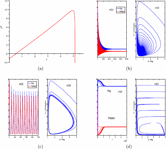

  

  Graph of function $S_{0}$ (a). The positive equilibrium $E^{*}$ of system (1.2) is stable when $\tau=0.4$ (b), $\tau=5.4$ (d), and unstable when $\tau=0.6$ (c). The other parameter values are $r=0.11$, $K=10$, $\beta=0.3$, $a=0.12$, $h_{1}=0.01$, $h_{2}=0.01$, $m=0.15$, $\theta=6$, and $\varepsilon=0.7$. The initial condition for panels (b) and (c) is $x_{0}=8$, $y_{0}=5$. Multiple initial conditions are used for panels (d)

• (1c) For $\tau=0.6\in(\tau^{*}, \tau^{**})$, the positive equilibrium of system (1.2) is unstable and there is a Hopf bifurcation when $\tau=\tau^{*}$ (see Fig. 2(c)).

• (1d) For $\tau=5.1\in(\tau^{**}, \tau_{\mathrm{max}})$, the positive equilibrium of system (1.2) is stable (see Fig. 2(d)).

For parameter set (ii), we have $\tau^{*}\approx1$ (see Fig. 3(a)).

• (2a) For $\tau=0$, the positive equilibrium of system (1.1) is stable (see Fig. 1(a)).

• (2b) For $\tau=0.9<\tau^{*}$, the positive equilibrium of system (1.2) is stable (see Fig. 3(b)).

  Figure 3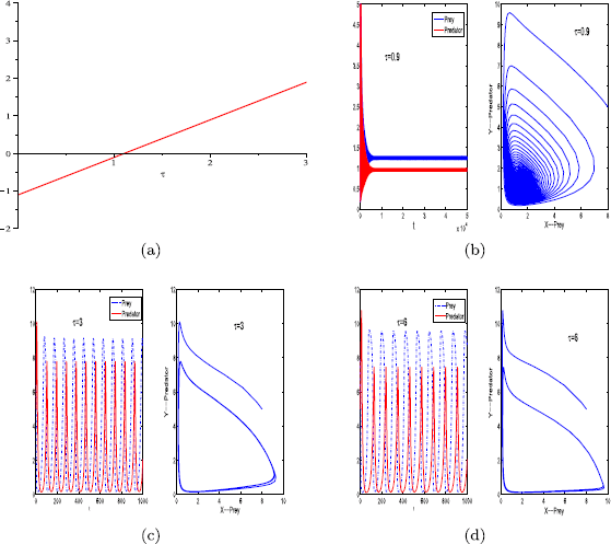

  

  Graph of function $S_{0}$ (a). The positive equilibrium $E^{*}$ of system (1.2) is stable when $\tau=0.9$ (b), and unstable when $\tau=3$ (c), $\tau=6$ (d). The other parameter values are $r=0.11$, $K=10$, $\beta=0.3$, $a=0.12$, $h_{1}=0.01$, $h_{2}=0.01$, $m=0$, $\theta=6$, and $\varepsilon=0.7$. Here the initial condition is $x_{0}=8$, $y_{0}=5$

• (2c) For $\tau=3.6>\tau^{*}$, the positive equilibrium of system (1.2) is unstable (see Fig. 3(c), (d)).

For parameter set (iii), we obtain $\tau_{\mathrm{max}}\approx3.27$ and $I=[0, 3.27)$. The graph of function $S_{0}(\tau)$ for $\tau\in I$ is displayed in Fig. 4(a). As indicated in Fig. 4(a), there is only one positive critical value of the delay τ, denoted by $\tau^{*}$. Here, $\tau^{*}\approx2.4$.

• (3a) For $\tau=0$, as indicated in Fig. 1(b), the positive equilibrium of system (1.1) is unstable.

• (3b) For $\tau=1$, $2<\tau^{*}$, the positive equilibrium of system (1.2) is unstable (see Fig. 4(b), (c)).

  Figure 4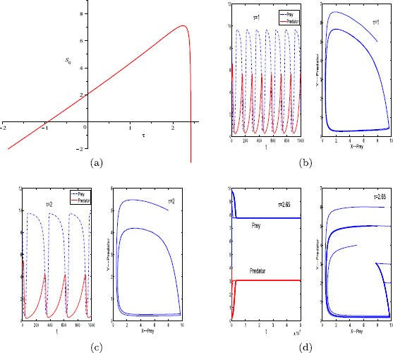

  

  Graph of function $S_{0}$ (a). The positive equilibrium $E^{*}$ of system (1.2) is unstable when $\tau=1$ (b), $\tau=2.65$ (d), and stable when $\tau=2$ (c). The other parameter values are $r=0.11$, $K=10$, $\beta=0.2$, $a=0.12$, $h_{1}=0.01$, $h_{2}=0.01$, $m=0.15$, $\theta=6$, and $\varepsilon=0.7$. The initial condition for panels (b) and (c) is $x_{0}=8$, $y_{0}=5$. Multiple initial conditions are used for panels (d)

• (3c) For $\tau=2.65\in(\tau^{*}, \tau_{\mathrm{max}})$, the positive equilibrium of system (1.2) is stable and there is a Hopf bifurcation when $\tau=\tau^{*}$ (see Fig. 4(d)).

For parameter set (iv), as shown in Fig. 5(a), there are no positive critical values of the delay τ.

• (4a) When $\tau=0$, as indicated in Fig. 1(b), the positive equilibrium of system (1.1) is unstable.

• (4b) When $\tau=1, 2.65, 10$, the positive equilibrium of system (1.2) is always unstable (see Fig. 5(b), (c), (d)).

  Figure 5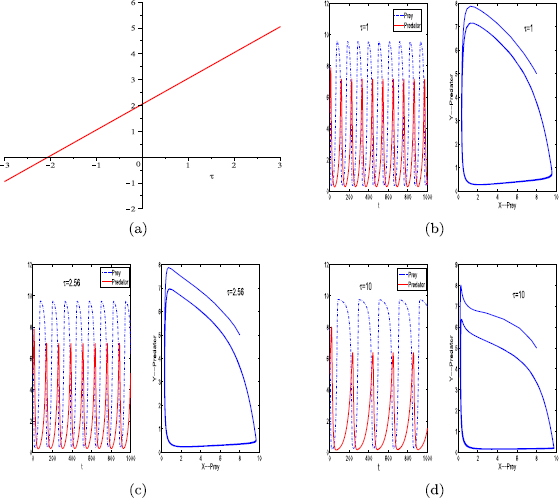

  

  Graph of function $S_{0}$ (a). The positive equilibrium $E^{*}$ of system (1.2) is always unstable when $\tau=1$ (b), $\tau=2.56$, (c) or $\tau=10$ (d). The other parameter values are $r=0.11$, $K=10$, $\beta=0.2$, $a=0.12$, $h_{1}=0.01$, $h_{2}=0.01$, $m=0$, $\theta=6$, and $\varepsilon=0.7$. Here, the initial condition is $x_{0}=8$, $y_{0}=5$

Bifurcation diagram Fig. 6 shows the evolution of the dynamics of system (1.2) for $m=0$ with the variation of time delay. For small time delay τ, the interior equilibrium of the system is stable. The stability of the interior equilibrium changes at $\tau \approx1$. As indicated in the figure, for large τ, the interior equilibrium is no longer stable and the system displays cycling behaviors.

Figure 6

Bifurcation diagram of system (1.2) with the variation of delay τ for $r=0.11$, $K=10$, $\beta=0.3$, $a=0.12$, $h_{1}=0.01$, $h_{2}=0.01$, $m=0$, $\theta=6$, and $\varepsilon=0.7$

6 Conclusions

In conclusion, the positive equilibrium of DDEs with delay-dependent coefficient displays stability switches and is ultimately stable under some conditions, indicating that a long delay stabilizes the interior equilibrium [18]. However, a DDEs model without delay-dependent coefficient usually behaves differently.

References

Holling, C.S.: Some characteristics of simple types of predation and parasitism. Can. Entomol. 91, 385–398 (1959)
Hassell, M.P., May, R.M.: Stability in insect host–parasite models. J. Anim. Ecol. 42, 693–726 (1973)
Smith, J.M.: Models in Ecology. Cambridge University Press, Cambridge (1974)
Hassell, M.P.: The Dynamics of Arthropod Predator–Prey Systems. Princeton University Press, Princeton (1978)
Ji, L.L., Wu, C.Q.: Qualitative analysis of a predator–prey model with constant-rate prey harvesting incorporating a constant prey refuge. Nonlinear Anal., Real World Appl. 11, 2285–2295 (2010)
Wang, S.L., Ge, Z.H.: The Hopf bifurcation for a predator–prey system with θ-logistic growth and prey refuge. Abstr. Appl. Anal. 2013, Article ID 168340 (2013)
Sih, A.: Prey refuges and predator–prey stability. Theor. Popul. Biol. 31, 1–12 (1987)
Taylor, R.J.: Predation. Chapman & Hall, New York (1984)
González-Olivares, E., Ramos-Jiliberto, R.: Dynamic consequences of prey refuges in a simple model system: more prey, fewer predators and enhanced stability. Ecol. Model. 166, 135–146 (2003)
Krivan, V.: Effects of optimal antipredator behavior of prey on predator–prey dynamics: the role of refuges. Theor. Popul. Biol. 53, 131–142 (1998)
Ma, Z.H., Li, W.L., Zhao, Y., Wang, W.T., Zhang, H., Li, Z.Z.: Effects of prey refuges on a predator–prey model with a class of functional responses: the role of refuges. Math. Biosci. 218(2), 73–79 (2009)
Chen, L.J., Chen, F.D., Chen, L.J.: Qualitative analysis of a predator–prey model with Holling type II functional response incorporating a constant prey refuge. Nonlinear Anal., Real World Appl. 11, 246–252 (2010)
Tao, Y.D., Wang, X., Song, X.Y.: Effect of prey refuge on a harvested predator–prey model with generalized functional response. Commun. Nonlinear Sci. Numer. Simul. 16, 1052–1059 (2010)
Tsoularis, A., Wallace, J.: Analysis of logistic growth models. Math. Biosci. 179, 21–55 (2002)
Wonlyul, K., Kimun, R.: A qualitative study on general Gause-type predator–prey models with constant diffusion rates. J. Math. Anal. Appl. 344, 217–230 (2008)
Hale, J.K.: Theory of Functional Differential Equations. Springer, Heidelberg (1977)
Wang, S.L., Wang, S.L., Song, X.Y.: Hopf bifurcation analysis in a delayed oncolytic virus dynamics with continuous control. Nonlinear Dyn. 67, 629–640 (2012)
Beretta, E., Kuang, Y.: Geometric stability switch criteria in delay differential systems with delay dependent parameters. SIAM J. Math. Anal. 33, 1144–1165 (2002)
Dieuonné, J.: Foundations of Modern Analysis. Academic Press, New York (1960)
Acknowledgements
This work is supported by NSFC (No. 11326200, No. 31470641), Foundation of He’nan Educational Committee (No. 15A110015), and the Grant of China Scholarship Council (No. 201408410018).
Author information
Authors and Affiliations
Contributions
All authors read and approved the final manuscript.
Corresponding author
Ethics declarations
Competing interests
The authors declare that they have no competing interests.
Additional information
Publisher’s Note
Springer Nature remains neutral with regard to jurisdictional claims in published maps and institutional affiliations.
Rights and permissions
Open Access This article is distributed under the terms of the Creative Commons Attribution 4.0 International License (http://creativecommons.org/licenses/by/4.0/), which permits unrestricted use, distribution, and reproduction in any medium, provided you give appropriate credit to the original author(s) and the source, provide a link to the Creative Commons license, and indicate if changes were made.
About this article
Cite this article
Xie, B., Xu, F. Stability analysis for a time-delayed nonlinear predator–prey model. Adv Differ Equ 2018, 122 (2018). https://doi.org/10.1186/s13662-018-1564-4
Received:
Accepted:
Published:
DOI: https://doi.org/10.1186/s13662-018-1564-4