
Abstract
In this paper, a novel automatic segmentation and reconstruction method is proposed for diffraction contrast tomography (DCT) technology. The pipeline of the proposed method starts from the imaging of Al−La alloy with the LabDCT technique from Carl Zeiss AG, which produces a sequence of 2D microstructure sections. Then, a segmentation algorithm based on superpixel and lifted multicut is proposed to extract the 2D microstructure in an image section. Finally, 2D segmentations are joined together to reconstruct and visualize the 3D microstructure. As a result, a novel morphology of Al−La alloy is recovered with both dendrite and lamellar morphologies. The proposed method has the advantage of the ability to losslessly recover the internal microstructure.
1 Introduction
It is important for researchers in materials domain to analyze the microstructures, which play an important role in the properties and performance of materials [1]. This analysis includes not only visualization but also quantitative evaluation of varying microstructures of materials. As a result, researchers have been always looking forward to a technique that is able to extract the complete microstructrue of grains losslessly. Actually, diffraction contrast tomography has been applied in material domain. Marrow et al. [2] used DCT to map the three-dimensional microstructure of a ceramic. McDonald et al. [3] made use of DCT to help understand how the densification of a powder body was affected by various factors, such as particle rearrangement, rotation, local deformation and diffusion, and grain growth. However, this technique has not been widely employed in material domain due to limitation of accuracy and inconvenience. Moreover, lack of automatic segmentation algorithm also hinders the development of microstructure analysis. Generally, microstructures of most grains are in a scale of micrometer, while a thousandfold microscope produces large and high-resolution images in a scale of millimeter. As a result, microscopic images often contain tens of thousands of grains, which is infeasible for manual labeling. Therefore, it increases the demand for efficient segmentation algorithms.
To alleviate this problem, many algorithms have been proposed to segment grain images with computer. Ullah et al. [4, 5] introduced a computer-aided method to accelerate the manual procedure. They designed a pipeline to segment the grain images with help of the software “imageJ”. First, all images were aligned using the a “Align3_TP”, one of the ImageJ plugins, to avoid tanslation and rotational displacements between consecutive sections. Then, pre-processing of images was conducted to select region of interest, correct uneven illuminated background, and remove the small spots. It was followed by a watershed algorithm and Geodesic transformation to obtain the 3D segmentation. Later, Waggoner et al. [6] presented an interactive propagating method to improve the segmenting quality. Their idea is to partition an image with help of the prior of the previous segmentation result, namely “information propagation”. As a result, a sequence of images can be segmented by repeatedly propagating this kind of segmentation from one slice to another. Hence, an interactive graphcut algorithm was introduced. However, human labeling was still necessary.
In this paper, the segmentation and reconstruction of 3D microstructure of the Al−La dendrite is investigated. Actually, many researchers have paid much attention to the microstructure of dendrites in Al−La alloy. The basic idea is to model the relationship between the microstructure and the properties of Al−La alloys. Zheng and Wang [7] reported a novel microstructure, periodic diphase dendrite in Al−35%La binary alloy. They found that there is a discontinuous microstructure in Al−35%La, which appears as a section plan crossed over some branches of tree-like structure. Then, Zheng et al. [8] experimentally studied the microstructure evolution of Al−La alloys with varying La contents. By ways of X-ray diffraction, field-emission scanning electron microscope, energy-dispersive spectrometer and tensile test, the variation of 2D microstructure of Al11La3 under different temperatures are discovered. Yang et al. [9] has reported that the appropriate addition of La had an advantages in refining grain size, removing harmful impurity, and improving tensile strength and elongation rate of aluminum alloys. Then, He et al. [10] looked into the progress of microstructure evolution of Al−La alloys with varying La contents. They found that the Al11La3 phase has an obvious influence on tensile strength, and La content has a greater effect on the plasticity of Al−La alloy. Therefore, the dendrites microstructure has important effect on the properties of Al−La alloys. However, all above studies focused on the 2D image rather than the 3D microstructure of the Al11La3 phase.
For the purpose of analyzing microstructures of Al11La3, the DCT technology is introduced in company with a lifted multicut segmentation algorithm. As a result, a complete 3D Al11La3 grain is, for the first time, reconstructed non-destructively. With the help of the visualization of the reconstructed grain we find that the dendrite structure, different from common dendrite of single phase, possess a novel 3D morphology. This is the reason why the chemical composition crossing the arms of the diphase dendrite changes in discontinuous and periodic oscillatory, which is consistent with the conclusion drawn by [7, 8].
The remaining of the paper is organized as following. Section 2 describes the segmentation algorithm. Subsequently, analysis of the segmentation algorithm and the resulted 3D microstructures are presented in Section 3. Conclusions are drawn in the final Section 4.
2 Methods
From the DCT image sequences of Fig. 1, we find that the 2D grains in a section appears like long strips crossing each other. Moreover, there is remarkable interval between two grains. Therefore, it is reasonable to employ segmentation algorithms in computer vision domain to separate different grains. In this paper, we formulate the segmentation of microstructure as a lifted multicut problem.

Image sections of 3d Al−La alloy
2.1 Segmentation as LMP
The minimum cost multicut problem (MP) is often used in image decomposition problem and it is equivalent to the graph decomposition problem. However, it models only pairs of neighboring nodes in the graph, which has difficulty in case of ambiguous boundaries. In order to differentiate the ambiguous boundaries, minimum cost lifted multicut problem (LMP) [11] is proposed to explicitly model relation between nodes that are not adjacent to each other. Therefore, the relationship between nodes around ambiguous boundaries can be separated with help of more information. This distinct makes feasible the segmentation of images with vague edges.
Before the introduction of LMP, we first give some parameters of LMP as follows.
-
A connected graph ζ=(V,E) with V the set of vertices, and E the set of edges associating with two neighbor vertices in V.
-
A graph ζ′=(V,E′), which is called the lifted graph of ζ, satisfies that E⊂E′, and D=E′∖E contains edges associating only with vertices that are not neighboring. It is remarkable that the graph ζ′ is an extension of ζ. In fact, when ζ′∖ζ=∅, there is no edge associating with vertices that are not neighboring. The LMP is reduced to MP problem. On the other hand, when ζ′∖ζ≠∅, LMP is not equivalent to MP. In this case, however, the solutions of MP and LMP are one-to-one corresponding.
-
A cost ce is assigned to every edge e∈E′, where e=uv connects two nodes u and v that belong to distinct components.
Subsequently, the minimum cost lifted multicut problem is defined as [11]:
where b∈B is a configuration of all the edge labeling in E′ that be∈{0,1}, and \(B \subseteq \{0, 1\}^{E^{\prime }}\) is the feasible set of the labeling configurations. In this optimization problem, the constrant (2) guarantees that the solution is feasible. It means that any solution set {e∈E|be=1} of (1) corresponds to a multicut or decomposition of G. While the constraints (3) and (4) ensure that for any edge e∈E′, be=0 if and only there is a path in ζ with all edges labeled 0; be=1 if and only if there is a cut in ζ with all edges labeled 1.
2.2 Implementation
The pipeline of the segmentation and reconstruction is shown in Fig. 2.
-
1.
Superpixel. To avoid the heavy computational cost, this paper constructs the lifted graph based on the super-pixel algorithm. The term superpixel denotes a set of neighboring image pixels that have similar visual characteristics. A number of algorithms [12] can be used to generate superpixels. As suggested by Stutz et al. [12] and Wang et al. [13], the super-pixel algorithms over-segment the image meshes into much smaller graphs, which greatly reduces the complexity of the following segmentation procedure. As images captured from DCT are always of high resolution, super-pixel algorithms improves the feasibility of the multicut problem.
Fig. 2 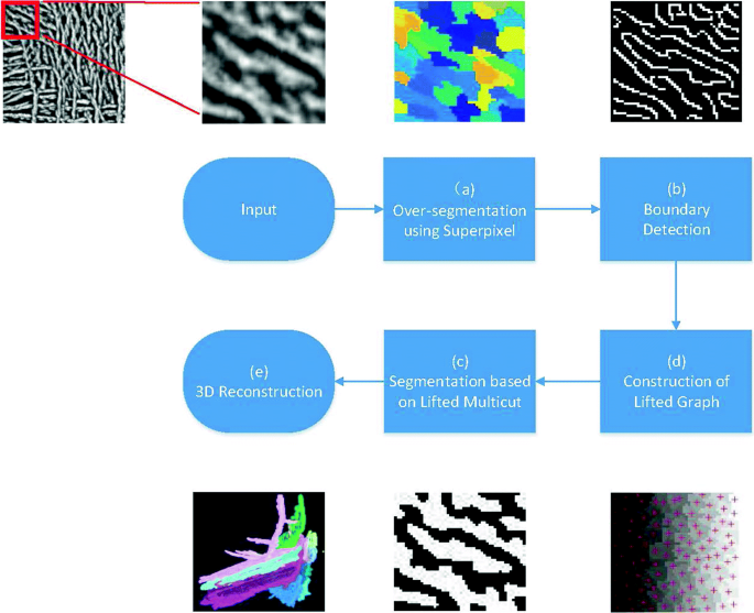
Illustration of the pipeline of the lifted multicut segmentation and reconstruction
Based on the super-pixel algorithm, an image is decomposed into a graph ζ.
-
2.
Boundary detection. It helps LMP determine the feature of an edge. Given \(\{d^{i}_{uv}\}, i=1,\ldots, n\) the set of detected boundaries between u and v, with di the strength of the i-th boundary point. The boundary feature can be determined by:
$$ f_{uv} = \frac{\sum_{i=1}^{n} d_{i}}{n} $$(5) -
3.
Construction of lifted graph. Moreover, a feature vector f is calculated for each node in ζ, which consists of the size, the gray histogram, skewness, kurtosis, maximum, minimum, sum, variance, etc.
According to the Bayesian Network, the cost ce depends on the conditional probability of \(y \in \{ 0, 1\}^{E^{\prime }} \) with respect to the feature vector x of an edge that [11]
$$ c_{e} = \text{log} \frac{1- p_{y|x}(1, x)}{p_{y|x}(1, x)}. $$(6)in which py|x can be estimated by logistic regression. However, there are two cases to consider the feature vector x. For the first case, an edge e∈E connects two neighboring nodes u and v of two different components. The feature vector of an edge is constructed by concatenating feature vectors of two nodes and the boundary feature between them.
As a result, the feature vector of an edge connecting u and v is constructed as xuv=[fu,fv,fuv].
Then, logistic regression is conducted based on xuv, which outputs the probability py|x that
$$ p_{y|x} = \frac{1}{1+\exp^{-\{\beta_{0} + \beta_{1} x \}}} $$(7)where β0 and β1 can be learnt from the training set.
For the other case, the two nodes of an edge e′ are not neighbors. It is equivalent to find a path that “best” connects these two nodes. However, it is different from and more difficult than the first case that it has to enumerate all paths connecting the two nodes. In this paper, the Dijkstra’s algorithm is used to find this path. After the path is obtained, its probability can be determined by:
$$ p_{y|x^{\prime}}(0, x^{\prime}) = \max_{P\in uv-paths(\zeta)} \prod_{e\in P} p_{y|x}(0, x). $$(8) -
4.
3D reconstruction. To construct the 3D microstructure of Al−La dendrite, it is necessary to join together all the 2D segmentation results. For this purpose, a 3D graph is introduced as following. Given two neighboring graphs ζl=(Vl,El) and ζl+1=(Vl+1,El+1) of the l-th layer and the l+1-th layer respectively, the cross-layer edge set can be defined as F={euv|u∈Vlandv∈Vl+1}. Moreover, the 3D graph can be defined as:
$$\begin{array}{@{}rcl@{}} &&\Gamma = (\Upsilon, \Xi) \\ \text{where }&& V \subset \Upsilon, \qquad \Xi = E \cup F. \end{array} $$(9)As far as the authors know, there have been many algorithms to obtain the solution of 3D graph [11, 14]. In the situation of DCT sequential images of Al−La dendrite, however, due to the tiny interval between two neighbor layers, the movement of a dendrite is always so slow that it is easy to interrelate two cross-layer dendrite according to the euclidean distance. Therefore, the cross-layer edge set is constructed as:
$$ F=\{e_{uv} | \frac{\sum_{u\cap v} 1}{\sum_{u\cup v} 1} > \epsilon, u\in V^{l}\text{and} v\in V^{l+1}\}. $$(10)where ε denotes the threshold that can be determined by experiments.

3 Discussion and experimental results
3.1 Dataset
To capture the microstructure of the alloy, this paper conducts diffraction constrast tomography experiments for Al−La alloy. The Xradia 510 Versa from Carl Zeiss AG is used in this test. As a result, a total number of 400 DCT sections are captured with interval of 2 microns between adjacent layers. The size of each section is 800×800 and each pixel has a resolution of 2×2 square microns. Example sections are shown in Fig. 1. To reduce the computational cost, each section is cropped into 4 images of 200×200. Therefore, a dataset of 6400 images is constructed for evaluation. For each image, the Al11La3 phase is manually labeled. Furthermore for all experiments in this section, the leave-one-out strategy is used and the dataset is split into 10 subsets.
3.2 Evaluation of superpixel
To evaluate the superpixel algorithms, we make use of the measurement of undersegmentation error (UE) [15] and boundary recall (Rec) [16] to evaluate. Suppose a region from the ground truth segmentation is Gi and from the superpixel algorithm is Sj. Then, the “leakage” is used here to describe the overlap of superpixels with multiple, nearby ground truth segments. It can be evaluated by:
where the normalized “leakage” of superpixel Sj with respect to Gi is denoted by \( \frac {\left (\sum _{S_{j} \cap G_{i} \neq \emptyset } |S_{j}|\right) -|G_{i}| }{|G_{i}|}\). A high value of UE means that the superpixels do not tightly fit the ground truth result. Rec evaluates the boundary with respect to the ground truth that:
where TP(G,S) means the number of true positive boundary pixels FN(G,S) denotes the number of false-negative boundary pixels. Therefore, a high Rec indicates better boundary detection.
We compare three superpixel algorithms, i.e., NC [17], Reg [18], and SLIC [15]. The evaluation results of these algorithms are shown in Fig. 3, from which we can draw three conclusions. Firstly, with the increase of number of superpixels, Rec results of the three algorithms are improved consistently. This is in tune with intuition that more superpixels lead to a less “leakage” and a better “fit”. Secondly, SLIC obtains the best results over the other two algorithms. Finally and most importantly, the cut-off number of superpixel, with satisfied performance, can be determined to be 1000. Actually, the Rec result of SLIC tends to be 1 when the number superpixels is more than 1000. NC gets a similar Rec with SLIC when the number of superpixels is more than 1300. In contrast, Reg obtains the worst result. Similarly, the UE curve of SLIC decreases nearly to the minimum, 0.72, after the number superpixels reaches 1000, while the best UE results of Reg and NC are 0.105 and 0.13 respectively.

Qualitative evaluation of superpixel algorithms on the DCT image dataset
3.3 Evaluation of boundary detection
Similar to superpixel, boundary also plays an important role in the cost of LMP (7). This section evaluates and chooses the most appropriate boundary detector for DCT images. Three boundary detectors are involved for comparison, i.e., DeepContour (DC) [19], Structure Forest (SF) [20]) and RCF [21]. The precision-recall curve is introduced to evaluate the performance of the three algorithms. Precision/recall curves are shown in Fig. 4. It indicates that the SF outperforms all the other two methods. In fact, SF obtains an F-score approximate to 0.69, while the F-scores of DC and RCF are 0.62 and 0.66 respectively.

Precision-recall curve
It should be noted that Fig. 4 does not mean disappointed performance of DeepContour and RCF. On other dataset, BSDS500 for example, we also obtain different results which support RCF. However, comprehensive evaluation of these algorithms is beyond the scope of this paper. Therefore, the objective conclusion is that the Structure Forest algorithm performs the best on our DCT dataset.
3.4 Performance of segmentation
This section evaluates the performance of LMP-based segmentation with different superpixel and boundary detection algorithms. We evaluate the influence of the two procedures, superpixel and edge detection, to the segmentation. The idea is to evaluate one procedure by fixing the other. Particularly, we choose structure forest as boundary detection method when assessing superpixel algorithms, because structure forest obtains the best performance in Section 3.3. Similarly, SLIC is employed as superpixel method when assessing boundary detection algorithms. As a result, a total of five combinations are compared: (1) NC [17] + SF [20], (2) Reg [18] + SF [20], (3) SLIC [15] + SF [20], (4) SLIC [15] + DC [19], and (5) SLIC [15] + RCF [21]. The number of superpixels is fixed to be 1000 due to the best performance in Fig. 3. All above combinations are followed by the logistic regression and the lifted multicut algorithm.
We introduce three indicators [22] in this evaluation, i.e., the segmentation covering (SC), the probabilistic Rand index (RI), and the variation of information (VI).
-
SC measures averaged matching between proposed segments with a ground truth labeling, defined as:
$$ SC(S, G) = \sum_{s_{i} \in S} \frac{|s_{i}|}{|G|} \max_{g_{j}\in G} \frac{s_{i} \cap g_{j}}{s_{i} \cup g_{j}} $$(13) -
Rand index (RI) evaluates the labeling distance between two regions, which is defined as:
$$ RI(S, G) = \sum_{i< j} \gamma_{ij} \Bigg/ \left(\begin{array}{cc} |G| \\ 2 \end{array} \right) $$(14)where:
$$ \gamma_{ij} = \left\{ \begin{array}{ll} 1 & \text{if there exist } {k} \text{ and } k^{\prime} \text{ such that both } x_{i} \text{ and }\\ & x_{j} \text{ are in both } s_{k} \text{ and } g_{k^{\prime}}\\ 1 & \text{if there exist } {k} \text{ and } k^{\prime} \text{ such that both } x_{i} \text{ is in,} \\ & \text{ both } s_{k} \text{ and } g_{k^{\prime}} \text{ and } x_{j} \text{ is in neither } s_{k} \text{ nor } g_{k^{\prime}} \\ 0 & \text{otherwise} \end{array} \right. $$(15) -
VI measures the relative entropy between two segmentation sets, S and G, and is defined as:
$$ VI(S, G) = H(S | G)+ H(G | S) $$(16)where H(S|G) and H(G|S) are conditional image entropies that can be defined as:
$$ H(S | G) = \sum_{l_{s}\in \{0,1\}} \sum_{l_{g}\in \{0,1\}} P(l_{s}, l_{g}) \log\frac{P(l_{g})}{P(l_{s},l_{g})} $$(17)where ls and lg are labels in S and G respectively. H(G|S) can be defined similarly.
The segmentation results using these three indicators are shown in Table 1. We can draw two conclusions. Firstly, the influence of superpixel is greater than that of boundary detector. The max deviation of SC is 0.18 (NC+SF) when alternating superpixel algorithms and 0.26 (SLIC+RCF) when alternating boundary detectors. Similar results can also be found in RI (0.219 vs 0.008) and VI (0.742 vs 0.043). This is reasonable because the accuracy of superpixel is the precondition of segmentation. Secondly, SLC + SF obtains the best performance in both SC and RI, and a similar performance with the best one (SLC + RCF). Therefore, this paper considers the combination SLC + SF as the best pipeline.
Subsequently, this paper analyzes the construction of the 3D graph. The only parameter in this procedure to be considered is the threshold ε in 10. For this evaluation, the cross-layer correspondences are manually labeled to construct the cross-layer edge set Fg. Given the cross-layer edge set Fs from the segmentation algorithm, the accuracy can be evaluated by:
where TP denotes the number of edges in Fg∩Fs, and GT denotes the number of edges in Fg. The results are shown in Fig. 5. It indicates that the accuracy keeps higher than 0.98 until ε>0.8. Therefore in this paper, the threshold is set to be 0.8.

Accuracy of cross-layer construction along with variation of the threshold
Finally, the 3D visualization technology allows us to investigate the microstructure of this dendrite in any view angle. This is illustrated in Fig. 6 where two observations are shown. This morphology has two features. First, the whole microstructure is well developed in the form of dendrite. For example in the left of Fig. 6, the dendrite structure appears as the base of the whole microstructure. On the other hand, the dendrite arm acts as lamellar eutectic morphology.

Different views of the dendrite of the phase Al11La3 in Al−La alloy. Different colors denote different connected components
The reconstructed three-dimentional microstructure in Fig. 6 is novel and different from the tree-structure described in [8]. Through 2D imaging methods ofX-ray diffraction and SEM, Zheng et al. [7, 8] found the diphase morphology in 2D images, which is predicted to produced by cross-sectioning the alloy vertical to dendrite arms (c.f. Fig. 4 in [8]). However, they did not verify this prediction without the complete three-dimensional microstructure. With help of the reconstructed three-dimensional microstructure in this paper, nevertheless, the 2D “diphase” dendrites named by Zheng et al. [8] are formulated by cross-sectioning the dendrites arms in lamellar eutectic microstructure.
4 Conclusion
While many researches focused on the variation of microstructure evolution [10] and properties of the alloy [9, 23] according to varying components, there has been little experimental verification of these microstructures in three dimension. For the Al−35La alloy prepared by free solidification experiment, the 3D dendritic microstructure of Al11La3 phase has been captured and analyzed based on the diffraction contrast tomography (DCT) technique and the lifted multicut algorithm.
The pipeline of the segmentation of DCT images consists of four procedures. The first one is the superpixel method, which greatly reduces the burden of segmentation. Then, the lifted graph is constructed based on the superpixels and boundary detection algorithms. It is followed by the lifted multicut algorithm which solves the image segmentation problem. After the experimental evaluation, the combination of SLIC [15] and SF [20] is selected to obtain the best segmenting accuracy. Finally, with help of the cross-layer correspondence and 3D visualization, the whole microstructure of Al11La3 is reconstructed from the DCT image sequence. As a consequence, a novel morphology of the Al11La3 phase is observed through the visualization of the 3D microstructure.
The value of this work is reflected in that, for the first time, the 3D microstructure is exhibited in the material domain. Moreover, compared to traditional mechanical cross-sectioning methods, the DCT technique as well as the LMP segmentation algorithm is able to recover the microstructure losslessly. Therefore, it is our future work to study the 3D microstructures of other kinds of alloys as well as their relationship to mechanical properties [10].
Abbreviations
- DC:
-
DeepContour
- DCT:
-
Diffraction contrast tomography
- FN:
-
False negative
- LMP:
-
Minimum cost lifted multicut problem
- MP:
-
Minimum cost multicut problem
- RCF:
-
Richer convolutional feature
- Rec:
-
Boundary recall
- RI:
-
Probabilistic rand index
- SC:
-
Segmentation covering
- SF:
-
Structure forest
- SLIC:
-
Simple linear iterative clustering
- TP:
-
True positive
- UE:
-
Undersegmentation error
- VI:
-
Variation of information
References
M.-n. Feng, Y.-c. Wang, H. Wang, G.-q. Liu, W.-h. Xue, Reconstruction of three-dimensional grain structure in polycrystalline iron via an interactive segmentation method. Int. J. Miner. Metall. Mater.24(3), 257–263 (2017).
T.J. Marrow, A. King, P. Reischig, S. Rolland Du Roscoat, W. Ludwig, Diffraction contrast tomography of polycrystalline alumina. Mater. Sci. Technol. Conf. Exhibition.1:, 489–499 (2009).
S.A. McDonald, C. Holzner, E.M. Lauridsen, P. Reischig, A.P. Merkle, P.J. Withers, Microstructural evolution during sintering of copper particles studied by laboratory diffraction contrast tomography (LabDCT). Sci. Rep.7(1) (2017).
A. Ullah, G. Liu, J. Luan, W. Li, M. ur Rahman, M. Ali, Three-dimensional visualization and quantitative characterization of grains in polycrystalline iron. Mater. Charact.91:, 65–75 (2014).
A. Ullah, G. Liu, H. Wang, M. Khan, D.F. Khan, J. Luan, Optimal approach of three-dimensional microstructure reconstructions and visualizations. Mater. Express.3(2), 109–118 (2013).
J. Waggoner, Y. Zhou, J. Simmons, M. De Graef, S. Wang, 3D materials image segmentation by 2D propagation: A graph-cut approach considering homomorphism. IEEE Trans. Image Process.22(12), 5282–5293 (2013).
Y. Zheng, Z. Wang, A novel periodic dendrite microstructure in Al-La binary alloy. J. Cryst. Growth.318(1), 1013–1015 (2011).
Y. H. Zheng, Z. D. Wang, S. M. Zhang, Microstructure of diphase dendrite in Al-35%La alloy during solidification. J. Cryst. Growth.362:, 33–37 (2013).
Q. Yang, F. Bu, F. Meng, X. Qiu, D. Zhang, T. Zheng, X. Liu, J. Meng, The improved effects by the combinative addition of lanthanum and samarium on the microstructures and the tensile properties of high-pressure die-cast Mg-4Al-based alloy. Mater. Sci. Eng. A. 628:, 319–326 (2015).
Y. He, J. Liu, S. Qiu, Z. Deng, J. Zhang, Y. Shen, Microstructure evolution and mechanical properties of Al-La alloys with varying La contents. Mater. Sci. Eng. A. 701:, 134–142 (2017).
M. Keuper, E. Levinkov, N. Bonneel, G. Lavoue, T. Brox, B. Andres, in International Conference on Computer Vision, Vol. 2015 Inter. Efficient decomposition of image and mesh graphs by lifted multicuts (IEEE, 2015), pp. 1751–1759.
D. Stutz, A. Hermans, B. Leibe, Superpixels: An evaluation of the state-of-the-art. Comp. Vision Image Underst.166:, 1–27 (2018).
M. Wang, X. Liu, Y. Gao, X. Ma, N.Q. Soomro, Superpixel segmentation: A benchmark. Signal Proc. Image Commun.56:, 28–39 (2017).
T. Liu, M. Zhang, M. Javanmardi, N. Ramesh, T. Tasdizen, in European Conference on Computer Vision. SSHMT: Semi-supervised Hierarchical Merge Tree for Electron Microscopy Image Segmentation (Springer, 2016), pp. 144–159.
R. Achanta, A. Shaji, K. Smith, A. Lucchi, P. Fua, S. Susstrunk, SLIC Superpixels Compared to State-of-the-Art Superpixel Methods. IEEE Trans. Pattern Anal. Mach. Intell.34(11), 2274–2282 (2012).
D.R. Martin, C.C. Fowlkes, J. Malik, Learning to detect natural image boundaries using local brightness, color, and texture cues. IEEE Trans. Pattern Anal. Mach. Intell.26(5), 530–549 (2004).
G. Mori, in International Conference on Computer Vision, Vol. II. Guiding model search using segmentation (IEEE, 2005), pp. 1417–1423.
H. Fu, X. Cao, D. Tang, Y. Han, D. Xu, Regularity preserved superpixels and super voxels. IEEE Trans. Multimedia. 16(4), 1165–1175 (2014).
W. Shen, X. Wang, Y. Wang, X. Bai, Z. Zhang, in Computer Vision and Pattern Recognition, Vol. 07-12-June. DeepContour: A deep convolutional feature learned by positive-sharing loss for contour detection (IEEE, 2015), pp. 3982–3991.
P. Dollar, C. L. Zitnick, in International Conference on Computer Vision. Structured forests for fast edge detection (IEEE, 2013), pp. 1841–1848.
Y. Liu, M.M. Cheng, X. Hu, K. Wang, X. Bai, in Computer Vision and Pattern Recognition. Richer convolutional features for edge detection (IEEE, 2017), pp. 5872–5881.
P. Arbeláez, M. Maire, C. Fowlkes, J. Malik, Contour detection and hierarchical image segmentation. IEEE Trans. Pattern. Anal. Mach. Intell.33(5), 898–916 (2011).
M. Murashkin, I. Sabirov, A. Medvedev, N. Enikeev, W. Lefebvre, R. Valiev, X. Sauvage, Mechanical and electrical properties of an ultrafine grained Al-8.5 wt. % RE (RE = 5.4 wt.% Ce, 3.1 wt.% La) alloy processed by severe plastic deformation. Mater. Des.90:, 433–442 (2016).
Acknowledgements
The author thanks the editor and anonymous reviewers for their helpful comments and valuable suggestions.
Funding
This work was partially supported by National Key Research and Development Program of China (No. 2016YFB0700500).
Availability of data and materials
I can provide the data.
Author information
Authors and Affiliations
Contributions
The author took part in the discussion of the work described in this paper. The author read and approved the final manuscript.
Corresponding author
Ethics declarations
Ethics approval and consent to participate
Approved.
Consent for publication
Approved.
Competing interests
There is no potential competing interests in our paper. The author has seen the manuscript and approved to submit to your journal. I confirm that the content of the manuscript has not been published or submitted for publication elsewhere.
Publisher’s Note
Springer Nature remains neutral with regard to jurisdictional claims in published maps and institutional affiliations.
Additional information
Authors’ information
Ya Su received the B.Sc., M.Sc., and Ph.D. degrees in Signal and Information Processing all from Xidian University, Xi’an, China, in 2003, 2006, and 2010 respectively. He was a Postdoc fellow at the State Key Laboratory of Intelligent Technology and Systems, Department of Electronic Engineering, Tsinghua University, Beijing, China. He is now faculty of the School of Computer and Communication Engineering, University of Science and Technology Beijing. His research interests include machine learning and computer vision.
Rights and permissions
Open Access This article is distributed under the terms of the Creative Commons Attribution 4.0 International License (http://creativecommons.org/licenses/by/4.0/), which permits unrestricted use, distribution, and reproduction in any medium, provided you give appropriate credit to the original author(s) and the source, provide a link to the Creative Commons license, and indicate if changes were made.
About this article

Cite this article
Su, Y. Segmentation and reconstruction of DCT images based on lifted multicut. J Image Video Proc. 2018, 135 (2018). https://doi.org/10.1186/s13640-018-0378-3
Received:
Accepted:
Published:
DOI: https://doi.org/10.1186/s13640-018-0378-3