Piano multipitch estimation using sparse coding embedded deep learning

Abstract

As the foundation of many applications, multipitch estimation problem has always been the focus of acoustic music processing; however, existing algorithms perform deficiently due to its complexity. In this paper, we employ deep learning to address piano multipitch estimation problem by proposing MPENet based on a novel multimodal sparse incoherent non-negative matrix factorization (NMF) layer. This layer originates from a multimodal NMF problem with Lorentzian-BlockFrobenius sparsity constraint and incoherentness regularization. Experiments show that MPENet achieves state-of-the-art performance (83.65% F-measure for polyphony level 6) on RAND subset of MAPS dataset. MPENet enables NMF to do online learning and accomplishes multi-label classification by using only monophonic samples as training data. In addition, our layer algorithms can be easily modified and redeveloped for a wide variety of problems.

1 Introduction

Multipitch estimation problem (MPE, cf. [1–4] and references therein) is the concurrent identification of multiple notes in an acoustic polyphonic music clip. For example, {C₄,D₄}, {E₀,G₂,A₅}, {F₃,A₃,C₄,E₄,G₄,B₄,D₅}¹, or other combinations. Generally, it is a prerequisite for Automatic Music Transcription (AMT, [5]), Musical Information Retrieval (MIR, [6]), and many other acoustic music processing applications. It is worth emphasizing that MPE is different from Automatic Chord Estimation (ACE, [7]) in two aspects: (1) note combinations in MPE can be totally random instead of certain relationships in ACE and (2) MPE is a multi-label classification [8] problem while ACE is a single-label one.

One challenge of MPE is overlapping partials [9, 10] (the spectra of different notes share many common frequency bins with each other). It is an inevitable result caused by temperament relationships and vibration properties. For example, Table 1 gives the frequency relationship between the first 30 overtones of a reference note and its upper octave under exact equal temperament assumption. Given a reference note n and its fundamental frequency f, denoting semitone shifts as subscripts, the fundamental frequency of n’s fifth note (seven semitones above n), for instance, is $f_{7} = f \times 2^{\frac {7}{12}}$. According to the equal temperament, the interval from f₇’s first octave to f’s third overtone is about 2 cents ($1200 * \log _{2} \left (\frac {3f}{2f_{7}}\right)\approx 2$, refer to the 9th row of Table 1). Analogically, we have the interval from f₃’s fourth octave to f’s 19th overtone is about − 2 cents ($1200 * \log _{2} \left (\frac {19f}{2^{4} f_{3}} \right) \approx -\thinspace 2$, refer to the 4th row of Table 1). One can easily testify the rest of the table.

Table 1 Frequency relationships between the overtones of a reference note n and its upper octave

Besides, the acoustical characteristics of different instruments make the problem even more difficult: on the one hand, timbre variation results in different overtone magnitude distributions; on the other hand, inharmonicity² leads to various overtone frequency distributions [11]. Pianos are especially harder to deal with than other stringed instruments due to the complicated way of strings being wired. Due to the inharmonicity and its uniqueness on different strings [11], the slight frequency mismatch between the first overtone of a note and its upper octave will cause an interference pattern (a.k.a. acoustic beat) if pianos are tuned by exact equal temperament. In order to eliminate such acoustic beats, pianos are usually tuned individually by well-trained experts (called harmonic tuning, the deviation from the exact equal temperament often forms a Railsback curve [12]).

The other challenge of MPE comes from the complexity of note combination. Strategies for solving multi-label classification can be generally categorized into two, “one vs. all” and “one vs. one,” respectively. Let the class number be n, the former needs n classifiers while the latter needs $\left (\begin {array}{cc}n\\2\end {array}\right) = \frac {n^{2} - n}{2}$ones. Although it is computationally feasible for most circumstances, classifiers are trained independently from feature extraction. The lack of supervision in feature extraction may degrade the performance since it is more meaningful for features to minimize classification error rather than reconstruction error [13]. Another existing strategy needs 2ⁿ classifiers by encoding multi-labels into single-labels. It is only feasible when n is not large; otherwise, one may suffer from dimension explosion problem. Taking the piano for example, choosing 7 notes from 88 yields $\left (\begin {array}{cc}88\\7\end {array}\right) \approx 6.3\times 10^{9}$ combinations. Even if only timbre and decay are included, it is almost impossible to construct and train such a large-scale dataset.

Moreover, as one of the most commonly used features in acoustic music processing applications, time-frequency representation is constrained by the uncertainty principle. The algorithm performance then may be degraded by such deficient feature. Meanwhile, recent results have shown that feature fusion from different sensors (namely modality, one may consider someone’s fingerprint and iris, or footages of some action from different angles) has advantages for recognition tasks (cf. [14–16] and references therein). Combined information from multiple sources is more robust and tolerant to noises and errors. Multimodal joint representation under constraints maximizes the utility of different features, which can be used more effectively in task-driven scenarios. Note that multimodal features are different from stacking multiple features into one because the latter does not take the modality relationship into account, and increasing dimensionality brings huge computation and storage costs.

Based on and inspired by the above discussion, we in this paper propose MPENet, which is a deep learning (DL, [17–21]) network enhanced by a novel multimodal sparse incoherent NMF layer (MSI-NMF layer). MPENet and MSI-NMF layer are implemented by Caffe [22]. Structures of training and test phase are given in Figs. 1 and 2, where tensors (i.e., Caffe blobs) are denoted by arrows, Caffe built-in layers are denoted by rectangles (computation) and ellipses (loss), layer collections by hexagons, our implemented layers by rounded rectangles. “Mod,” “cod,” and “pred” are abbreviations for modality, coding, and prediction, respectively. Modality indices are appended by dashes. Repeated elements (represented by dashed lines) are omitted for simplicity purpose. Network details are explained in Sections 3 and 4. MPENet incorporates the supervision from data and task to train dictionaries and classifiers adaptively and jointly. Representative and discriminative features then can be used to make multi-label inference directly from superposed inputs. Our main contributions include:

• Lorentzian-BlockFrobenius sparsity: A novel $\| \cdot \|_{\mathcal {L}-BF, \gamma }$ is imposed to a multimodal NMF model. Penalty is determined by the magnitude of class templates of all modalities so that class sparsity can be ensured.

  Fig. 1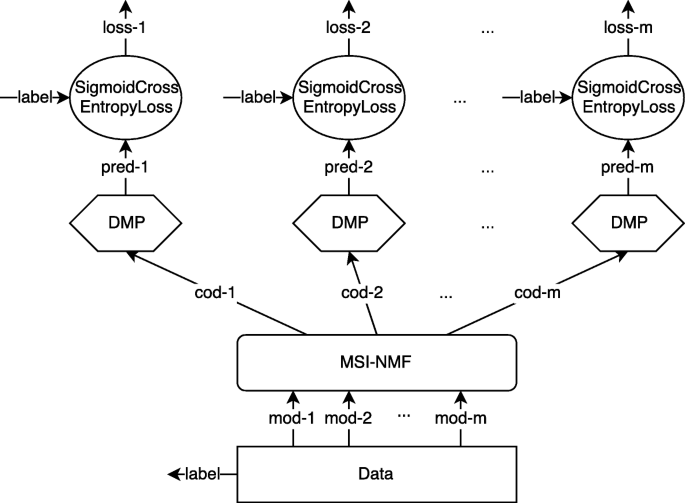

  

  Training structure of MPENet. Following Caffe terminology, this figure shows the computation graph of training phase. Arrows indicate blobs; rectangles and ellipses indicate Caffe built-in computation and loss layers. Hexagons indicate layer collections. Rounded rectangles indicate our implemented layers. All built-in layer names conform to Caffe. More details are explained in Sections 3 and 4. Repeated elements of each modality are omitted by dashed lines

  Fig. 2

  

  Test structure of MPENet. Following Caffe terminology, this figure shows the computation graph of test phase. Legends can be referred to Fig. 1. More details are explained in Sections 3 and 4

• Multimodal sparse incoherent NMF layer: A new deep learning layer based on the above constrained NMF model is presented. Sparse representations, as layer outputs, are computed by Alternating Direction Method of Multipliers (ADMM). Dictionaries, as layer parameters, are updated by Projected Stochastic Gradient Descent (PSGD). Incoherentness is added to the net loss as weight decay. Layer formulation and algorithms are given in Section 3.

• Multipitch estimation network (MPENet): Given the decomposition capability of proposed layer, we employ “one vs. all” strategy and present a unified deep learning network consisting of a training subnet and a test subnet. Experiments show that the test net achieves state-of-the-art results by using only two modalities of monophonic samples as training data. Network details are explained in Section 4.

2 Related work

Owing to the non-negativity and superposition properties of musical spectra, Non-negative Matrix Factorization (NMF, [23]) is applied widely in the latest acoustic music processing studies. Musical spectral data is decomposed into a dictionary and corresponding coefficients (also referred to as codings, activations, or activities in some references, we may use any of them according to the context). Note that NMF algorithms converge in unsupervised fashion, only rank-1 decomposition makes sense for computational stability and uniqueness purpose. Thus, most methods utilizing NMF employ a three-step procedure: (1) training note templates individually from samples of each note, (2) constructing a dictionary by concatenating all note templates, and (3) estimating multiple notes by computing the codings with the dictionary fixed. In early studies, each template has only one atom (columns of a dictionary are called atoms). Weninger et al. [24] develop this simple structure by dividing note samples into two parts: onset and decay. Then, two atoms are learned respectively from both parts, which yields a two-column note template. Such dictionary helps to capture the feature variation and distinguish note state over time. O’Hanlon and Plumbley [25] take a further step on dictionary flexibility. Note templates are constructed by using linear combinations of several pre-defined fixed narrow-band harmonic atoms. The input spectral data is then approximated under β-divergence group sparsity constraint. Other methods employing similar idea but different implementations are proposed in [2, 4, 26–29]. Such procedure uses fixed dictionary to get note activations during test, so MPE results heavily depend on the learned note templates, i.e., training samples. One has to retrain each template once new samples are added into training set. For other work using NMF with row/group sparsity and incoherent dictionaries, refer to [30–32] and references therein. Note that there are also studies that use unsupervised NMF instead of training note templates via isolated note samples. Bertin et al. [33] propose a tempering scheme favoring NMF with Itakura-Saito divergence to global minima. O’Hanlon and Sandler [34] propose an iterative hard thresholding approach for l₀ sparse NMF problem with Hellinger distance. ERBT spectrograms of polyphonic music pieces are decomposed directly and a pitch salience matrix is calculate to detect active notes. A semi-supervised NMF method can be referred to [35].

Many non-NMF based algorithms have been proposed for MPE problem. Tolonen and Karjalainen [36] divide the signal into two channels according to a fixed frequency and compute autocorrelation of the low channel and the envelope of the high channel to form summary autocorrelation function (SACF) and enhanced SACF (ESACF). The SACF and ESACF representations are used to observe the periodicities of the signal and estimate notes. Klapuri [37] calculates the salience representation through a weighted summation of overtone amplitudes. Three estimators based on direct, iterative, and joint strategies are proposed to extract notes from the salience function. Emiya et al. [1] employ a probabilistic spectral smoothness principle to iteratively estimate polyphonic content from a set of note candidates. An assumption of maximum number of concurrent notes (n_max=6) is imposed to avoid extracting overmany notes. Adalbjörnsson et al. [3] use a fixed dictionary to reconstruct input signal under block sparsity constraint. Notes are then identified through coding magnitudes. The fixed dictionary used here, however, is constructed according to equal-tempered scale so that the algorithm is unsuitable for instruments with inharmonicity.

Deep learning has been used to address AMT problem in recent papers. Sigtia et al. [38] presents a real-time model which introduces recurrent neural networks (RNN) into a convolutional neural network (CNN, with only convolution, pooling, and fully connected layers). Kelz et al. [39] compare the performances of networks with different types of inputs (spectrograms with linearly/logarithmically spaced bins, logarithmically scaled magnitude, and constant-Q transform), layers (dropout and batch normalization), and depths. Hawthorne et al. [40] propose a deep model with bidirectional long short term memory (BiLSTM) networks and two objective functions (onsets and frames), achieving state-of-the-art performance on MAPS [1] under configuration 2 described in [38]. For more acoustic music processing work using deep learning, refer to [40] and references therein. Note that the deep learning methods listed here all use music pieces as training data, which means polyphonic information can be accessed, hence music language model and classifiers are learned simultaneously.

3 Multimodal sparse incoherent NMF layer

3.1 Notation

Throughout this paper, we denote vectors and matrices by bold lowercase and uppercase letters, for example, $\mathbf {v} \in \mathbb {R}^{m}$ and $\mathbf {M} \in \mathbb {R}^{m \times n}$. Parts of vectors and matrices are denoted by subscripts: v_i is the i-th entry of v; M_i, M_i→, M_i,j, and M_i,j,p,q represent the i-th column, i-th row, (i, j)-th entry, and p×q block starting from (i, j)-th entry, respectively. 〈·,·〉 denotes the inner product of two vectors. For $p \geqslant 1$, the l_p norm of v is defined as $\| \mathbf {v} \|_{p} \triangleq \left (\sum _{i=1}^{m} | \mathbf {v}_{i} |^{p}\right)^{\frac {1}{p}}$, and the Frobenius norm of M as $\| \mathbf {M} \|_{F} \triangleq \left (\sum _{i, j} \mathbf {M}_{i,j}^{2}\right)^{\frac {1}{2}}$. Projection operator and indicator function of a set $\mathcal {C}$ with respect to a point x are respectively defined as

$$\Pi_{\mathcal{C}}(\mathbf{x}) \triangleq \underset{\mathbf{y} \in \mathcal{C}}{\text{argmin}} ~ \| \mathbf{y} - \mathbf{x} \|_{2}^{2}, \quad \delta_{\mathcal{C}}(\mathbf{x}) \triangleq \left\{\begin{array}{ll} 0, & \mathbf{x} \in \mathcal{C} \\ \infty, & \text{otherwise} \end{array}\right. $$

For notation simplicity, we also define $\mathbb {N}^{m} \triangleq \{1, 2, \ldots, m\}$, $\mathbb {R}_{\geqslant 0}\triangleq \{x|x \in \mathbb {R}, x \geqslant 0\}$.

3.2 Prototype

In comparison with other information fusion techniques, multimodal joint sparse representation provides an efficient tool and results in superior performance [41]. Redundancy is generally employed in dictionary learning algorithms [15, 42, 43] so that training data can be fit better and codings can be more discriminative and sparser. Besides, l_p,1 norm ([15]) is usually used to regularize codings for row sparsity, where

$$ \| \mathbf{M} \|_{l_{p,1}} \triangleq \sum\limits_{i = 1}^{d} \| \mathbf{M}_{i\rightarrow} \|_{p}, ~ \mathbf{M} \in \mathbb{R}^{d \times m}, ~ p \geqslant 1 $$

(1)

It enforces dictionaries of different modalities using same atom to present same event, for example, l_2,1 encourages collaboration among all modalities, and l_1,1 imposes extra sparsity within rows.

For MPE problem, dictionary incoherentness should be imposed to provide flexibility of modeling universal note representations in contrast to redundancy. As we discussed in Section 1, single-atom note templates cannot cover the diversity of music spectra whereas NMF cannot guarantee the stability and uniqueness for multi-atom ones. Because harmonic tuning aggravates overlapping partials, we can not distinguish that a spectral peak is a note overtone or a summation of several ones, i.e., it is not feasible to decompose frequency domain into orthogonal bins according to the center frequencies of harmonic series. In order to detect notes directly from factorization, a “good” dictionary should be trained under the supervision of data and task, possessing the following properties: (1) note templates are mutually discriminative and (2) for a certain note, all possible variants can be and only can be represented by its templates.

Moreover, we improve l_p,1 norm for two reasons. The first one is coding structure does not satisfy row-wise sparsity since dictionary incoherentness is imposed. Note samples are approximated by linear combination of its template atoms. The second one is l₁ norm imposes too much penalty so that every activation is either scaled down or zeroed out by soft threshold shrinkage [44]. For unknown number and loudness in MPE problem, each coding entry is crucial for detecting notes correctly, so we want to preserve as many effective activations as possible. Opposed to l₁ and l₂, the Lorentzian- l₂ norm [45]³, defined as

$$ \| \mathbf{v} \|_{\mathcal{L}-l_{2}, \gamma} \triangleq \sum\limits_{i = 1}^{d} \log \left(1 + \frac{\mathbf{v}_{i}^{2}}{\gamma^{2}} \right), ~ \mathbf{v} \in \mathbb{R}^{d}, ~ \gamma \geqslant 0 $$

(2)

penalizes large activations with small weights but the other way around so that non-zero activations keep their contributions. Besides, l₁ norm is not differentiable at 0, which makes the computation of gradient complicated ([15] tackles this by introducing “active set”). The everywhere smoothness of Lorentzian- l₂ provides good convergence property. Figure 3 shows the contours of several common regularizations.

Fig. 3

Contours of several norm regularizations are discussed here

Summing up the above discussion, the prototype of multimodal sparse incoherent NMF layer is a multimodal sparse incoherent NMF model whose cost function is, given multimodal input $\left \{\mathbf {x}^{i} \in \mathbb {R}_{\geqslant 0}^{f^{i}}, i=\mathbb {N}^{m}\right \}$,

$$\begin{array}{*{20}l} &{} l\left(\left\{\mathbf{D}^{i}\right\}, \mathbf{A}; \left\{\mathbf{x}^{i}\right\}\right) \triangleq \\ &{} \underset{\mathbf{A} \in \mathcal{A}, \mathbf{D}^{i} \in \mathcal{D}^{i}}{\text{min}} \sum\limits_{i = 1}^{m} \left(\frac{1}{2} \left\| \mathbf{D}^{i} \mathbf{A}_{i} - \mathbf{x}^{i} \right\|_{2}^{2} + \frac{\mu}{2} \sum\limits_{j = 1}^{d} \sum\limits_{k = 1, k \neq j}^{d} \left\langle \mathbf{D}^{i}_{j}, \mathbf{D}^{i}_{k} \right\rangle^{2} \right) \\ &{} + \lambda_{1} \| \mathbf{A} \|_{\mathcal{L}-BF, \gamma} + \frac{\lambda_{2}}{2} \| \mathbf{A} \|_{F}^{2}, ~ \mu > 0, \lambda_{1} > 0, \lambda_{2} > 0 \end{array} $$

(3)

where superscripts indicate modality indices, m denotes modality number, f denotes feature dimensionality, n denotes class number, a denotes atom number of each class template, d=n×a is dictionary column number, and {μ,λ₁,λ₂} are penalties. $\mathcal {A} \triangleq \left \{ \mathbf {M} | \mathbf {M} \in \mathbb {R}_{\geqslant 0}^{d \times m} \right \}$ is coding space; $\mathcal {D}^{i} \triangleq \left \{ \mathbf {N} | \mathbf {N} \in \mathbb {R}_{\geqslant 0}^{f^{i} \times d}, \| \mathbf {N}_{j} \|_{2} \leqslant 1, j = \mathbb {N}^{d}\right \}$ are dictionary spaces. Lorentzian-BlockFrobenius norm is defined as

$${} \|\! \mathbf{A} \!\|_{\mathcal{L}-BF, \gamma} \!\triangleq\! \sum\limits_{i = 1}^{n} \!\log\!\left(\!1 \!\,+\, \frac{\| \mathbf{A}_{i\Box} \|_{F}^{2}}{\gamma^{2}}\!\right)\!\!, \!\mathbf{A}_{i\Box}\! \triangleq\! \mathbf{A}_{(i-1)a +\! 1, 1, a, m}\!,\! \gamma \!>\!\! 0 $$

In (3), A_i□ contains all template coefficients of the i-th class of all modalities. Frobenius norm incorporates the contributions of different modalities. Thus, Lorentzian-BlockFrobenius norm imposes class sparsity instead of row sparsity. The inner product term enforces that the dictionary columns have the least coherentness. It ensures the discrimination among class templates as well as the linear representation within each template. Note that analytic or straight optimization cannot be done for (3) because it is not jointly convex with respect to (w.r.t) $\left \{\mathbf {D}^{i}, i = \mathbb {N}^{m}\right \}$ and A. It is convex w.r.t either one while the other fixed. Hence, many alternating schemes ([42, 44, 46, 47]) split (3) into two subproblems, sparse coding and dictionary learning, respectively.

3.3 Structure

MSI-NMF layer is constructed by re-translating the two subproblems of (3), where we treat A as layer outputs and $\left \{\mathbf {D}^{i}, i = \mathbb {N}^{m}\right \}$ as layer parameters. Using the same network notations as in Section 1, Fig. 4 shows the structure of MSI-NMF layer, where layer parameters are denoted by texts within parentheses.

Fig. 4

Structure of MSI-NMF layer. Legends can be referred to Fig. 1. Following Caffe terminology, arrows indicate tensors (Caffe blobs), and dictionaries ($\mathbf {D}^{i}, i = \mathbb {N}^{m}$) are treated as layer parameters

3.4 Forward pass

The forward pass produces the solution of a multimodal non-negative sparse coding problem whose cost function is defined as

$$\begin{array}{*{20}l} l_{f}\left(\mathbf{A}; \left\{\mathbf{x}^{i}, \mathbf{D}^{i}\right\}\right) \triangleq & \underset{\mathbf{A} \in \mathcal{A} }{\text{min}} ~ \frac{1}{2} \sum_{i = 1}^{m}\left\|\mathbf{D}^{i} \mathbf{A}_{i} - \mathbf{x}^{i}\right\|_{2}^{2} \\ & + \lambda_{1} \| \mathbf{A} \|_{\mathcal{L}-BF, \gamma} + \frac{\lambda_{2}}{2} \| \mathbf{A} \|_{F}^{2} \end{array} $$

(4)

To solve (4), let $f = \sum _{i=1}^{m} f^{i}$, define $\mathbf {D} \in \mathbb {R}_{\geqslant 0}^{f \times md}$, $\mathbf {a} \in \mathbb {R}_{\geqslant 0}^{md}$, and $\mathbf {x} \in \mathbb {R}_{\geqslant 0}^{f}$

$$\mathbf{D} \triangleq \left(\begin{array}{llll} \mathbf{D}^{1} & & & \\ & \mathbf{D}^{2} & & \\ & & \ddots & \\ & & & \mathbf{D}^{m} \end{array}\right), ~~ \mathbf{a} \triangleq \left(\begin{array}{c} \mathbf{A}_{1} \\ \mathbf{A}_{2} \\ \vdots \\ \mathbf{A}_{m} \end{array}\right), ~~ \mathbf{x} \triangleq \left(\begin{array}{c} \mathbf{x}^{1} \\ \mathbf{x}^{2} \\ \vdots \\ \mathbf{x}^{m} \end{array}\right) $$

Then, (4) can be rewritten as

$$ {}l_{f}(\mathbf{a}; \mathbf{x}, \mathbf{D}) \triangleq \underset{\mathbf{a} \in \mathbb{R}_{\geqslant 0}^{md} }{\text{min}} ~ \frac{1}{2} \| \mathbf{D} \mathbf{a} - \mathbf{x} \|_{2}^{2} + \lambda_{1} \| \mathbf{a} \|_{\mathcal{L}-bl_{2}, \gamma} + \frac{\lambda_{2}}{2} \| \mathbf{a} \|_{2}^{2} $$

(5)

where

$$ \| \mathbf{a} \|_{\mathcal{L}-bl_{2}, \gamma} \triangleq \sum_{i = 1}^{n} \log \left(1 + \frac{\tilde{\mathbf{a} }_{i} }{\gamma^{2}} \right) $$

(6)

$$ {\kern35pt}\tilde{\mathbf{a} }_{i} = \sum_{j=1}^{m} \sum_{k = 1}^{a} \mathbf{a}^{2}_{(j-1)d + (i-1)a + k} $$

(7)

(5) can be solved using Alternating Direction Method of Multipliers (ADMM, ref. [44, 46, 47]), details are given in Algorithm 1 (proofs in Appendix), where Φ is given in Algorithm 2.

3.5 Backward pass

The backward pass is to update D through gradient descent. The incoherentness constraint is treated as weight decay of layer parameters. Denoting the network cost function by l_net, the new cost function becomes

$$ l_{\text{new}} \triangleq l_{\text{net}} + \frac{\mu}{2} \sum\limits_{i = 1}^{m} \left(\sum\limits_{j = 1}^{d} \sum\limits_{k = 1, k \neq j}^{d} \left\langle \mathbf{D}^{i}_{j}, \mathbf{D}^{i}_{k} \right\rangle^{2}\right) $$

(8)

Then, we have

$$ {}\frac{\partial l_{\text{new}}}{\partial \mathbf{D}_{p, q}} = \frac{\partial l_{\text{net}}}{\partial \mathbf{D}_{p, q}} + \frac{\mu}{2} \frac{\partial {\sum\nolimits}_{i = 1}^{m} \left({\sum\nolimits}_{j = 1}^{d} {\sum\nolimits}_{k = 1, k \neq j}^{d} \left\langle \mathbf{D}^{i}_{j}, \mathbf{D}^{i}_{k} \right\rangle^{2}\right)}{\partial \mathbf{D}_{p, q}} $$

(9)

where $p = \mathbb {N}^{f}, q = \mathbb {N}^{md}$. According to the chain rule, the first term of (9) is

$$ \frac{\partial l_{\text{net}}}{\partial \mathbf{D}_{p, q}} = \left\langle \frac{\partial l_{\text{net}}}{\partial \mathbf{a}}, \frac{\partial \mathbf{a} }{\partial \mathbf{D}_{p, q}} \right\rangle $$

(10)

In order to get $\frac {\partial \mathbf {a} }{\partial \mathbf {D}_{p, q}}$, recalling that a is a minimizer of (5), taking the derivative w.r.t a, we have

$$ \mathbf{D}^{\mathsf{T}}(\mathbf{D} \mathbf{a} - \mathbf{x}) + \lambda_{1} \tilde{\mathbf{W}} \mathbf{a} + \lambda_{2} \mathbf{a} = \mathbf{0} $$

(11)

where $\tilde {\mathbf {W}} = \Psi (\mathbf {a})$ is defined as

$$\begin{array}{*{20}l} \tilde{\mathbf{W}} & = \left(\begin{array}{llll} \mathbf{W} & & & \\ & \mathbf{W} & & \\ & & \ddots & \\ & & & \mathbf{W} \end{array}\right) \end{array} $$

(13)

$$\begin{array}{*{20}l} \mathbf{W} & = \left(\begin{array}{llll} w_{1} \mathbf{I} & & & \\ & w_{2} \mathbf{I} & & \\ & & \ddots & \\ & & & w_{n} \mathbf{I} \end{array}\right) \end{array} $$

(14)

$$\begin{array}{*{20}l} w_{i} & = \frac{2}{\gamma^{2} + \tilde{\mathbf{a}}_{i} }, \quad i = \mathbb{N}^{n} \end{array} $$

(15)

$\tilde {\mathbf {a}}$ is defined in (7). Then, $\frac {\partial l_{\text {new}} }{ \partial \mathbf {D}_{p, q} }$ can be computed because $\frac {\partial \mathbf {a} }{\partial \mathbf {D}_{p, q}}$ can be obtained by taking the derivative w.r.t D_p,q on (11) and $\frac {\partial l_{\text {net}} }{ \partial \mathbf {a} }$ is given by the last layer.

The backward algorithm of proposed layer is listed in Algorithm 3 (proofs in Appendix), where $\mathbf {V}^{i} \in \mathbb {R}^{d \times n}$ is defined as

$$ \mathbf{V}^{i} \triangleq \left(\begin{array}{llll} \mathbf{A}_{1,i,a,1} & & & \\ & \mathbf{A}_{a + 1,i,a,1} & & \\ & & \ddots & \\ & & & \mathbf{A}_{(n -1)a + 1,i,a,1} \end{array}\right) $$

(16)

$i = \mathbb {N}^{m}$, diag(M) is a diagonal matrix whose diagonal entries come from M, and $\mathbf {U}^{i} \in \mathbb {R}^{d \times d}$.

4 MPENet

In this section, we detailedly explain the layer and tensor specifics of MPENet. In order to avoid misunderstandings caused by layer names in different deep learning frameworks (for example, commonly called “fully connected” is named as “inner product” in Caffe, “linear” in PyTorch, and “dense” in TensorFlow), during illustration, we will give the mathematics expression of some layers if necessary. Meanwhile, in order to give the most direct ideas of how MPENet is constructed, we switch to Caffe terminology accordingly (see Figs. 1 and 2).

In Figs. 1 and 2, training and test phases have same core modules, differences only locate in the top layers. “Data” layer produces multimodal features and their labels. Labels are binary vectors whose entries are 1 if corresponding classes are active and 0 otherwise. “SigmoidCrossEntropyLoss” layer is a stack of “sigmoid” layer and “cross-entropy” layer. Cross-entropy loss is defined as

$$-\frac{1}{n} \sum\limits_{i=1}^{n}\left(\mathbf{p}_{i} \log \hat{\mathbf{p}}_{i} + \left(1 - \mathbf{p}_{i}\right) \log \left(1 - \hat{\mathbf{p}}_{i} \right)\right), \quad \mathbf{p}, \hat{\mathbf{p}} \in \mathbb{R}^{n} $$

where p and $\hat {\mathbf {p}}$ are predictions and labels.

4.1 Deep multi-label prediction module (DMP)

The structure of “Deep Multi-label Prediction” (DMP) is shown in Fig. 5. “Slicing” layer segments an n×a vector into n parts. “Detection” is a classifier module with replaceable structure, and is supposed to output the existence magnitude according to the input. “Concat” (concatenation) layer joints n detections to form a multi-label prediction. In our experiment, five layers are used to implement “Detection” module (structure is shown in Fig. 6). “InnerProduct” represents the transform from $\mathbf {x} \in \mathbb {R}^{m}$ to $\mathbf {y} \in \mathbb {R}^{n}$

$$\mathbf{y} = \mathbf{W} \mathbf{x} + \mathbf{b}, ~\mathbf{W} \in \mathbb{R}^{n \times m}, \mathbf{b} \in \mathbb{R}^{n} $$

“ReLU” (Rectified Linear Unit) stands for the transform from $\mathbf {x} \in \mathbb {R}^{m}$ to $\mathbf {y} \in \mathbb {R}^{m}$

$$\mathbf{y}_{i} = \text{max}(\mathbf{x}_{i}, 0), ~i=\mathbf{N}^{m} $$

For other tasks, one can modify this combination accordingly.

Fig. 5

Structure of “DMP.” Legends can be referred to Fig. 1. All built-in layer names conform to Caffe. Details can be referred to Section 4.1

Fig. 6

Structure of “Detection” implemented in our experiment. Legends can be referred to Fig. 1. All built-in layer names conform to Caffe. Details can be referred to Section 4.1

The reason for such structure roots from the property of incoherent dictionaries. If samples of certain class can be and only can be represented by its template atoms, the existence of this class is only related to the coefficient magnitudes. “One vs. all” strategy can be employed natively. If dictionaries are not as good as expected, cross-entropy loss will correct each “detection” module as well as dictionaries of the proposed layer through backward pass, which completes a positive circle.

4.2 Multi-label accuracy layer

Multi-label accuracy layer is implemented to conduct training and test in a unified framework. It consists of three sequential operations: sigmoid activation, binary output, and metric computation. The second one outputs either 0 or 1 according to the comparison result between the sigmoid activation and a predefined threshold t. The third one calculates the Precision (P), Recall (R), and F-measure (F) according to the binary outputs and the ground truths, where

$$P = \frac{TP}{TP + FP}, \quad R = \frac{TP}{TP + FN}, \quad F = \frac{2 \times P \times R}{P+R} $$

TP, FP, and FN stand for true positive, false positive, and false negative, respectively.

5 Experiment results

In this section, we first briefly demonstrate the dataset and features used in our experiment, then illustrate parameter initialization and network configuration in detail. Piano MPE results, experiment results about how MPENet works, timbre robustness results, and AMT results are given in the end of this section.

5.1 Dataset and features

MAPS [1] is a commonly used piano dataset for multipitch estimation and automatic transcription. It contains nine kinds of recording conditions (referred to as “StbgTGd2,” “AkPnBsdf,” “AkPnBcht,” “AkPnCGdD,” “AkPnStgb,” “SptkBGAm,” “SptkBGCl,” “ENSTDkAm,” and “ENSTDkCl”), two of them (“ENSTDkAm” and “ENSTDkCl”) are from real pianos and seven are synthesized by softwares. Each kind has same subset hierarchies which include ISOL (monophonic recordings), RAND (random combination), and UCHO (chords).

ISOL/NO subset, which contains 264 monophonic wav files covering 88 notes (n=88) and 3 loudness levels, is used as training set. RAND subset, which contains 6 polyphony levels ranging from 2 to 7 (labeled as P2–P7), is used as test set. Each one of P2–P7 has 50 files, and the note combination of each file is generated randomly. In [1], a 93-ms frame which is 10 ms after onset of each file in P2–P6 is analyzed. As comparison, we conduct similar evaluation in our experiment. P7 is used as validation set for parameter tuning.

Each wav file in MAPS is stereo with sampling rate 44100 Hz. To extract features, we firstly generate a mono counterpart by averaging both channels. Then, the silent part of each counterpart is truncated according to the provided onsets and offsets. Finally, two kinds of features (m=2) are extracted from the remainder by Short Time Fourier Transform (STFT) and Constant-Q Transform (CQT). The reason for using STFT and CQT is mainly because the former has good resolution in high-frequency domain while the latter does well in low-frequency domain. STFT and CQT features are further transformed into non-negative dB scale using

$$ h(\cdot) \triangleq \frac{\log_{10}(\cdot / \epsilon + 1)}{\log_{10}(1 / \epsilon + 1)} $$

(17)

where · is either CQT or STFT feature and ε is the machine precision. Other extraction specifics are listed in Table 2, where flen, slen, minf, maxf, dim, ppo, and nfft are abbreviations for frame length, step length, minimal frequency, maximal frequency, dimensionality, partition per octave, and n-point Fast Fourier Transform, respectively.

Table 2 Feature specifics used in MPENet

5.2 Parameter initialization

Due to the non-convexity of problem (3), only local minimization can be guaranteed. The initial value of dictionaries is crucial for convergence and performance. Since totally random initialization makes the codings of first several epochs meaningless, it is a waste of time and computation resources. Plus, because each monophonic file in the training set lasts for over 2 s, many samples are similar to each other during decay. It is not reasonable to initialize the dictionary using random samples as most dictionary learning algorithms do [15] either. In our experiment, two procedures are employed to initialize the dictionary.

To avoid the heavy overhead caused by joint learning of dictionaries and classifiers, before really getting into MPENet, we propose a pre-learning phase called Label Consistent Incoherent Dictionary Learning (LCIDL) derived from [48, 49] to obtain a better start than random initialization and sample initialization for dictionaries in MSI-NMF layer. The cost function of LCIDL is

$$\begin{array}{*{20}l} &{} l_{\text{lc}}\left(\left\{\mathbf{D}^{i}\right\}, \mathbf{A};\left\{\mathbf{x}^{i}\right\}\right) \triangleq \\ &{} \underset{\mathbf{A} \in \mathcal{A}, \mathbf{D}^{i} \in \mathcal{D}^{i}}{\text{min}} \sum_{i = 1}^{m} \left(\frac{1}{2} \left\| \mathbf{D}^{i} \mathbf{A}_{i} - \mathbf{x}^{i} \right\|_{2}^{2} + \frac{\mu}{2} \sum_{j = 1}^{d} \sum_{k = 1, k \neq j}^{d} \left\langle \mathbf{D}^{i}_{j}, \mathbf{D}^{i}_{k} \right\rangle^{2}\right) \\ &{}+ \lambda_{1} \| \mathbf{A} \|_{\mathcal{L}-BF, \gamma} + \frac{\lambda_{2}}{2} \| \mathbf{L} - \mathbf{A} \|_{F}^{2} \end{array} $$

(18)

where $\mathbf {L} \in \mathbb {R}^{d \times m}$ (referred to as discriminative coding) is, if $\left \{\mathbf {x}^{i}, i = \mathbb {N}^{m}\right \}$ belongs to the j-th note,

$$\mathbf{L} = \left(\begin{array}{c} \mathbf{L}_{1} \\ \vdots \\ \mathbf{L}_{n} \end{array}\right), \quad \mathbf{L}_{k} = \left\{\begin{array}{ll} \mathbf{1}^{a \times m}, & k = j \\ \mathbf{0}^{a \times m}, & \text{otherwise} \end{array}\right., \quad k = \mathbb{R}^{n} $$

It is worth emphasizing that (18) is a plain data-driven problem, and neither MPENet nor classifiers are involved at the time. It has nothing to do with deep learning and can be implemented by any language. The form of L is the extension of binary labels to impose classification information, because there are no note probabilities but only codings on our hands.

Likewise, LCIDL also needs a good dictionary to start for acceleration. In order to find it and determine the atom number, a fast clustering algorithm based on density peaks [50] is employed to filtrate samples hierarchically. Specifically speaking, we first extract 30 cluster centers from each modality of each file in the training set. Then, we stack them according to their note indices. This gives us two matrices with 810 columns for each note (810=30×3 (loudness) ×9 (recording)). Finally, through computing density peaks on these two matrices and considering the overhead and efficiency of computation and storage, we empirically set the atom number of each note template to be 15 (i.e., a=15 in (3)) and obtain a 576×1320 matrix and 648×1320 matrix for starting LCIDL.

After LCIDL is done, we obtain a “roughly good” dictionary, it has low reconstruction loss, incoherentness, and coding shape like L as (18) governs. When the real training of MPENet begins, this “roughly good” dictionary is copied into MSI-NMF layer, and classifiers are initialized randomly. During the first several epochs of training, the learning rate of classifiers is relatively larger than that of MSI-NMF since we want to hold codings a little bit to fit classifiers first. As the classification error decreases, the learning rates of all layers become equal to do joint learning.

5.3 Network configuration

Choices of parameters used in MPENet are all empirical. The output numbers of three “InnerProduct” layers in Fig. 6 are set to be 60, 30, and 1 from left to right. All three layers use bias term. For MSI-NMF layer, we use λ₁=0.15, λ₂=0.1, μ=1.32, ρ=0.2, γ=1.09, and t=0.5 for training. Considering that only one note is active at a time during training whereas at least two are active concurrently during test, test constraints should be weaker than those of training. Limited by the computation overhead, a fully greedy search cannot be done to get the best result. Therefore, we initialize several groups of parameters, and the one with λ₁=0.03, λ₂=0.1, μ=1.32, ρ=0.2, and γ=0.55 gets the best result through evaluating the test net on P7. To tune binary threshold t of multi-label accuracy layer, we plot a Precision-Recall Curve in Fig. 7 according to the evaluation result on P7, where t ranges from 0 to 1 with step 0.001. Through the figure, we find that “detection” modules produce very polarized outputs. The best result (91.37% Precision and 70.92% Recall, see the gray square in Fig. 7) and similar ones can be achieved when t is within a relatively large interval around 0.5. Therefore, we keep t=0.5 unchanged for test.

Fig. 7

Precision-Recall Curve of P7. “Detection” module produces similar results when t varies in a relatively large interval around 0.5, the best result is shown by a gray square

5.4 MPE results

Evaluation metrics are listed in Tables 3, 4, and 5 when the polyphony level is unknown. Our network outperforms all other algorithms on Recall and F-measure. Precisions of P2, P3, and P6 get the second best results with slight gaps compared to Emiya’s. The decrease of sparsity constraint is the reason for this result shortage. During evaluation, we can achieve over 99.9% F-measure for P2 and P3 if we use training parameters. Such configuration can also maintain high Precision results for P4–P6; however, Recall will drop dramatically due to strong sparsity. It is a trade off and contradiction between sparsity and concurrent notes.

Table 3 Precision (%) result with unknown polyphony level

Table 4 Recall (%) result with unknown polyphony level

Table 5 F-measure (%) result with unknown polyphony level

We also report the evaluation results in Table 6 when polyphony level is known as prior. For polyphony level k, we choose the indices of first k largest outputs in sigmoid layer as active notes. Results show that F-measure increases for P2 and P3 while things are different for P4–P6. It states a fact that when concurrent number is small, the ground truths have higher probabilities than others in our algorithm; as concurrent number grows, undetected ground truths become undetectable.

Table 6 F-measure (%) result with known polyphony level

5.5 How MPENet works

In order to show how each key part of MPENet contributes to the performance, we conduct four groups and seven in total experiments. Considering the combination complexity, each experiment only changes single part to show its impact on the system. Group indices, names, and settings are listed in Table 7, where √ and × indicate presence and absence, respectively; the setting described in Sections 5.3 and 5.4 is called MPENet-default (MPENet-d for short). Unless otherwise specified, all experiments in this subsection share same parameters with MPENet-d except the modified part. Implementation details and results are explained in the following subsections.

Table 7 Experiment settings for part comparison, where group 1 corresponds to modality variation only, group 2 to atom number, group 3 to joint learning, and group 4 to dictionary incoherentness

5.5.1 Modality

Config.1 and Config.2 use single modal features listed in Table 7 as training inputs to show our multimodal efficacy. Results are plotted in Fig. 8. We find that STFT’s Precision outperforms CQT’s on all test sets, while the STFT’s Recall decreases substantially from P3. MPENet-d, as expected, incorporates the advantages of both modalities and amend their drawbacks.

Fig. 8

Modality comparison results. Precision, Recall, and F-measure are shown in three subplots from top to bottom, respectively, where yaxis indicates percentage value and xaxis indicates polyphony level. Three subplots share same legends

5.5.2 Atom number

Group 2 (Config.3–Config.5), in conjunction with MPENet-d, shows the influence of atom number on our system. We only change a described in Section 5.2 to initialize dictionaries with different sizes. Results are plotted in Fig. 9. Interestingly, the Precision of each one in group 2 gets improvement except P2 of Config.4. Especially, the Precision increase of Config.5 (a=20) for all test sets and that of Config.3 (a=5) for P5–P6 are substantial. While the Recall for P2 are all close to each other, and Config.5’s Recall remains approximately equal to MPENet-d’s for P2–P5, Config.3’s Recall and Config.4’s (a=10) decrease a little. As a result, the F-measures of Config.3 for P2 and Config.5 for P2–P4 are slightly higher than that of MPENet-d. Such result implies that MPENet becomes robust to polyphony level under same parameters as atom number increases. We think the reason for oscillated metrics is parameters still have strong influences on the outputs in this situation. Although Config.5 performs better than MPENet-d for P2–P5, considering time complexity ($\propto \mathcal {O} \left (p m n^{2} \sqrt {\kappa _{\mathbf {D}^{\mathsf {T}} \mathbf {D} + \left (\rho + \lambda _{2}\right) \mathbf {I}}}\right)$ for conjugate gradient method or $\propto \mathcal {O} \left (p m n^{3} \right)$ for Cholesky decomposition method, where p is ADMM iteration number, κ is condition number, m,n,D are defined in (5)) and the F-measure of P6, we consider MPENet-d sufficient enough. For those with unlimited computation resources, one can modify a and re-validate corresponding parameters for better performances.

Fig. 9

Atom number comparison results. Precision, Recall, and F-measure are shown in three subplots from top to bottom, respectively, where y axis indicates percentage value andx axis indicates polyphony level. Three subplots share same legends

5.5.3 Joint learning

Config.6 (without joint learning) is implemented by dividing dictionary and classifier learning as separate operations. During training, we first learn dictionaries by using (18) in Section 5.2 since it is the only way to impose supervision. Then, we compute the codings of monophonic training data by using (4) with learned dictionaries. Finally, monophonic codings are directly fed into “dmp” modules plotted in Fig. 1 to train classifiers. During test, we first compute the codings of polyphonic test data in P2–P6, then use the test phase in Fig. 2 to get metrics. Note that dictionaries are only learned once and do not change any more during coding computation and classifier training. Comparison results are shown in Fig. 10, where we find that although Config.6 beats MPENet-d by 2% constantly on Precision, the Recall of Config.6 has increasing gap compared with MPENet-d’s as polyphony level grows. As a result, MPENet-d outperforms Config.6 greatly on F-measure for P4–P6.

Fig. 10

Joint learning comparison results. Precision, Recall, and F-measure are shown in three subplots from top to bottom, respectively, where y axis indicates percentage value and x axis indicates polyphony level. Three subplots share same legends

5.5.4 Dictionary incoherentness

For Config.7 (without dictionary incoherentness), we remove the incoherentness regularization in (3). Due to the absence of incoherentness, block sparsity makes no sense then. The cost function used in Config.7 becomes

$$\begin{array}{*{20}l} &{} l\left(\left\{\mathbf{D}^{i}\right\}, \mathbf{A}; \left\{\mathbf{x}^{i}\right\}\right) \triangleq \\ &{} \underset{\mathbf{A} \in \mathcal{A}, \mathbf{D}^{i} \in \mathcal{D}^{i}}{\text{min}} \sum\limits_{i = 1}^{m} \left(\! \frac{1}{2} \left\| \mathbf{D}^{i} \mathbf{A}_{i} - \mathbf{x}^{i} \right\|_{2}^{2} \right) \,+\, \lambda_{1} \| \mathbf{A} \|_{\mathcal{L}-rl_{2}, \gamma} \,+\, \frac{\lambda_{2}}{2} \| \mathbf{A} \|_{F}^{2} \end{array} $$

(19)

where Lorentzian-Row_ l₂ is defined as

$$\| \mathbf{A} \|_{\mathcal{L}-rl_{2}, \gamma} \triangleq \sum\limits_{i = 1}^{d} \log \left(1 + \frac{\| \mathbf{A}_{i\rightarrow} \|_{2}^{2}}{\gamma^{2}}\right) $$

The corresponding form of (18) then becomes

$$ \begin{aligned} l_{\text{lc}}\left(\left\{\mathbf{D}^{i} \right\}, \mathbf{A};\left\{\mathbf{x}^{i}\right\}\right) \triangleq & \underset{\mathbf{A} \in \mathcal{A}, \mathbf{D}^{i} \in \mathcal{D}^{i} }{\text{min}} \sum\limits_{i = 1}^{m} \left(\frac{1}{2} \left\| \mathbf{D}^{i} \mathbf{A}_{i} - \mathbf{x}^{i} \right\|_{2}^{2} \right) \\ & + \lambda_{1} \| \mathbf{A} \|_{\mathcal{L}-rl_{2}, \gamma} + \frac{\lambda_{2}}{2} \| \mathbf{L} - \mathbf{A} \|_{F}^{2} \end{aligned} $$

(20)

Forward and backward algorithm for (19) can be derived according to Algorithms 1 and 3. During training, we find the loss of training phase stays to a relatively high value (about two order higher than that of MPENet-d). Things do not change even if we reinitialize the parameters or train for extra several epochs. Moreover, during test, the sigmoid outputs of multi-label accuracy layer for P2–P6 are all less than the detection threshold t, so the metrics of Config.7 are all zero, test fails.

Summing up the results, we find that incoherentness regularization is crucial for MPENet while modality, atom number and joint learning only affect performance. If sorting them by importance, we have

$$\text{\footnotesize incoherentness} \gg \text{\footnotesize modality} \geqslant \text{\footnotesize joint learning} \geqslant \text{\footnotesize atom number} $$

5.6 Timbre robustness

In order to explore the generalization error of MPENet, another experiment is conducted by evaluating timbre robustness. In this experiment, we only choose “ENSTDkCl” as training set and test on other eight kinds. Parameter settings are all kept the same as in the last subsection. The reason for choosing “ENSTDkCl” is that it is recorded from a real piano with “close” recording condition. Inharmonicity, tuning, timbre, decay, background noise and all other factors that can influence spectra may be very different from the other eight. The results in Figs. 11, 12, and 13 show that MPENet becomes overfitting since all metrics of test sets drop fairly except “ENSTDkAm” (only recording condition is different from training set).

Fig. 11

Precision results of timbre robustness experiment

Fig. 12

Recall results of timbre robustness experiment

Fig. 13

F-measure results of timbre robustness experiment

5.7 AMT results

Due to the underlying strong relationship between MPE and AMT, and in order to further explore the capacity of MPENet, we also conduct AMT experiments following configuration 2 described in [38]. Specifically speaking, we use total 60 full-length music pieces contained in the “MUS” subsets of “ENSTDkCl” and “ENSTDkAm” as input and run MPENet frame by frame. Parameters and hyper-parameters are all kept the same as “MPENet-d” (c.f Sections 5.3 and 5.4). In line with the training phase of MPENet, the ground truths of music pieces are generated by discretizing note durations provided in corresponding txt files. Table 8 gives the frame-level average AMT results of MPENet, with comparison to state-of-the-art performance reported in [40]. MPENet maintains the Precision as in Section 5.4, but performs poorly on Recall. Figures 14 and 15 reveal some occasions where false positives and false negatives take place, in which green indicates true positives, red indicates false negatives and blue indicates false positives. In brief, false positives consist of a few wrong chord detections and many scattered unrelated notes; while false negatives come from massive so-called super-combinations (number of simultaneously active notes is over 7) and plenty of notes with long duration. The former circumstance of false negatives, as discussed in Section 5.4, is an inevitable result caused by sparsity constraints. For the latter circumstance of false negatives, however, we think the reasons behind such behaviors are mainly caused by two aspects: (1) the training set of MPENet lacks negative samples. Since training loss is not zero and recall the decay properties of piano notes, classification errors of monophonic samples in training set include wrong detections and missing detections. The lack of negative samples makes MPENet tend to distinguish the beginning from the end of same note, which leads to insufficient durations; (2) MPENet knows nothing about music language, which prevents MPENet from rejecting scattered, unreasonable detections.

Fig. 14

AMT results of the first 30 s of “MAPS_MUS-bk_xmas5_ENSTDkCl” produced by plain MPENet, where green indicates true positives, red indicates false negatives and blue indicates false positives. A typical case of false positives is extra note detection in some chords. A typical case of false negatives is where more than 7 notes are active simultaneously (MPENet can detect the attacks, but not the decays)

Fig. 15

AMT results of the first 30 s of “MAPS_MUS-deb_clai_ENSTDkCl” produced by plain MPENet, where legends can be referred to Fig. 14. A typical case of false negatives is where notes have long duration (still, MPENet can detect the attack of each note, but decays are discontinuous since the note probabilities are polarized caused by non-linear classifiers, c.f Fig. 7)

Table 8 Frame-level AMT results using 60 full-length music pieces in “ENSTDkCl/MUS” and “ENSTDkAm/MUS”

In order to compensate the second aspect discussed above and incorporate music prior with MPENet, we also train a simple recurrent network whose structure is given in Fig. 16. The training set follows the configuration 2 in [38], which consists of all music pieces in MAPS except the ones in “ENSTDkCl” and “ENSTDkAm”. The music context is constructed as follows: for a certain time step t, the recurrent network takes current binary label l_t as ground truth, and 16-time steps (about 100 ms) before and after it ({l_t−16,…,l_t−1,l_t+1,…,l_t+16}) as input. The number of hidden state in Gated Recurrent Units (GRU) is 200. The output number of all InnerProduct layers is 200 as well except the last one is 88 for label consistency. Before concatenation, we only keep the last step’s output of each GRU because they accumulate all the information through time. After the training is done, we use this recurrent network to perform Gibbs sampling on the sigmoid output of MPENet. If letting the total frame number of test dataset be N and running Gibbs sampling N times as one full step, we find that one full step gives the best performance improvement (1.81% on Precision and 0.11% on Recall). As expected (see Fig. 17 for example), the recurrent network smooths out some scattered detections. With more than one full step, however, the recurrent network breaks down the initial MPENet output and tends to “recompose” it into a new piece of music, which results in a major metrics decreasing. Note that indices of Gibbs sampling are selected randomly, so not all frames have been updated during one full step. Also note that our recurrent network has way shorter memory than those in [38, 40], so it learns little music language and only has effects on scatted detections. Because AMT is not the concern of this paper, we do not experiment more here but maybe focus on possible AMT-related refinements in the future work.

Fig. 16

Structure of the recurrent network used in AMT experiments. The inputs are 16 time steps before and after current label. The number of hidden state of GRUs is 200, the output numbers of InnerProducts are all 200 except the last one is 88. Before concatenation, we only keep the last step’s output of each GRU because they accumulate all the information through time. Legends can be referred to Fig. 1

Fig. 17

AMT results of the first 30 s of “MAPS_MUS-deb_clai_ENSTDkCl” after the regularization of recurrent network. Some false positives are smoothed out. Note that since Gibbs sampling indices are selected randomly, not all frames have been updated by the recurrent network

6 Conclusions

In this paper, we propose a new deep learning layer based on a NMF model with multimodal inputs under sparsity and incoherentness constraints. Such “layerization” of optimization problem provides the possibility to learn dictionaries and other features jointly under a unified deep learning framework. It enables modularization, online learning, and parameter fine-tuning for dictionary learning problem, which can be used to simplify the model refactoring and extension. In comparison with the “high level” features produced by other deep learning layers, the proposed layer learns discriminative and representative dictionaries so that the outputs are more realistically meaningful. Experiment results demonstrate that our test net improves the MPE performance substantially on MAPS dataset.

Restricted by hardwares, we pay more attention to layer algorithm and the network structure than model training. Unlike those fully explored and well-tuned deep learning models, MPENet with empirical parameters, simple layer combinations and shallow structures have plenty room for improvements. For future work, there are several directions that can be considered: (1) from the layer point of view, performance grows with the increasing modality number. According to our experiment results, automatic parameter adaptation will also improve the estimation greatly; (2) from the network point of view, regularization, depth, and structure are new focuses for extracting more representative and robust features.

7 Appendix

Proposition 1

a obtained by Algorithm 1 is a minimizer of (5).

Proof

Algorithm 1 is a straightforward application of ADMM. Introducing t, b and using the notation in 3.4, the unconstrained form of (5) is

$$ {}\frac{1}{2}\!\| \mathbf{D} \mathbf{t} - \mathbf{x} \|_{2}^{2} + \lambda_{1} \| \mathbf{a} \|_{\mathcal{L}-bl_{2}, \gamma} + \frac{\lambda_{2}}{2} \| \mathbf{t} \|_{2}^{2} + \frac{\rho}{2} \| \mathbf{t} - \mathbf{a} + \mathbf{b}\|_{2}^{2} + \delta_{\mathbb{R}^{md}_{\geqslant 0}}\!(\mathbf{a}) $$

(21)

Applying ADMM, the update scheme of (21) is

Solving (27) yields

$$\mathbf{t} = \left(\mathbf{D}^{\mathsf{T}}\mathbf{D} + (\rho + \lambda_{2})\mathbf{I}\right)^{-1}\left(\mathbf{D}^{\mathsf{T}} \mathbf{x} + \rho (\mathbf{a} - \mathbf{b})\right) $$

which is the update of t in Algorithm 1. To solve (28), we first change its form into

$$ \mathbf{a} = \underset{\mathbf{a}}{\text{min}}~ \frac{\lambda_{1}}{\rho} \| \mathbf{a} \|_{\mathcal{L}-bl_{2}, \gamma} + \frac{1}{2} \| \mathbf{t} - \mathbf{a} + \mathbf{b}\|_{2}^{2} +\delta_{\mathbb{R}^{md}_{\geqslant 0}}(\mathbf{a}) $$

(30)

Denoting $\lambda = \frac {\lambda _{1}}{\rho }$ and using Karush-Kuhn-Tucker conditions, we introduce $\mathbf {v} \in \mathbb {R}_{\geqslant 0}^{md}$. The Lagrange function of (30) is

$$ \mathcal{L}(\mathbf{a}, \mathbf{v}) \triangleq \lambda \| \mathbf{a} \|_{\mathcal{L}-bl_{2}, \gamma} + \frac{1}{2} \| \mathbf{t} - \mathbf{a} + \mathbf{b}\|_{2}^{2} - \langle \mathbf{v}, \mathbf{a} \rangle $$

(31)

and KKT conditions are

where $i = \mathbb {N}^{md}$ and $\tilde {\mathbf {W}}$ is defined in (13). It is easy to find (32) can be split into n independent groups

$$ (\lambda \mathbf{W} + \mathbf{I}) \mathbf{a}_{i\curvearrowright} = \mathbf{t}_{i\curvearrowright} + \mathbf{b}_{i\curvearrowright} + \mathbf{v}_{i\curvearrowright}, ~ i = \mathbb{N}^{n} $$

(36)

where

$$ {}\mathbf{a}_{i\curvearrowright} \triangleq \left(\begin{array}{c} \mathbf{a}_{(i, 1)\downarrow} \\ \vdots \\ \mathbf{a}_{(i, m)\downarrow} \end{array}\right), ~ \mathbf{a}_{(i, k)\downarrow} \triangleq \left(\begin{array}{c} \mathbf{a}_{(k - 1)d + (i-1)a + 1} \\ \vdots \\ \mathbf{a}_{(k - 1)d + ia} \end{array}\right)\!,\! ~ k = \mathbb{N}^{m} $$

(37)

and $\mathbf {t}_{i\curvearrowright }$, $\mathbf {b}_{i\curvearrowright }$, $\mathbf {v}_{i\curvearrowright }$ are defined accordingly. For any $i = \mathbb {N}^{n}$, we omit the subscript and let $\mathbf {a}' = \mathbf {a}_{i\curvearrowright }$ and $\mathbf {u}' = \mathbf {t}_{i\curvearrowright } + \mathbf {b}_{i\curvearrowright } + \mathbf {v}_{i\curvearrowright }$, we have equations

$$ \left\{\begin{array}{lc} \vdots \\ \frac{2\lambda}{\gamma^{2} + \| \mathbf{a}' \|_{2}^{2}} \mathbf{a}'_{j} + \mathbf{a}'_{j} = \mathbf{u}'_{j} \\ \vdots \\ \frac{2\lambda}{\gamma^{2} + \| \mathbf{a}' \|_{2}^{2}} \mathbf{a}'_{k} + \mathbf{a}'_{k} = \mathbf{u}'_{k} \\ \vdots \end{array}\right., \quad j,k = \mathbb{N}^{ma} $$

(38)

Through (38), we have a^′ and u^′ are collinear. Or one can get this conclusion more intuitively from a geometrical point of view through (31). In Fig. 18, for any a3∈{a | ∥a∥>∥u^′∥}, we have $\mathcal {L}(\mathbf {u}') < \mathcal {L}(\mathbf {a3})$; for any a2∈{a | 〈a,u^′〉≤0} we have $\mathcal {L}(\mathbf {0}) < \mathcal {L}(\mathbf {a2})$; for any a1∈{a | ∥a∥≤∥u^′∥,〈a,u^′〉>0}, a1 can be written as a1=a1_∥+a1_⊥ where a1_∥=hu^′,h>0 and 〈a1_⊥,u^′〉=0, one can testify that $\mathcal {L}(\mathbf {\mathbf {a1}_{\|}}) \leqslant \mathcal {L}(\mathbf {a1})$.

Fig. 18

Colinearity explanation of a^′ and u^′. Dashed lines indicate projections and dotted lines indicate the distance between two points

Setting a^′=βu^′,β∈[0,1], (30) can be rewritten as

$$ \beta = \underset{\beta \in [0, 1]}{\text{argmin}}~ \lambda \| \beta \mathbf{u}' \|_{\mathcal{L}-bl_{2}, \gamma} + \frac{\| \mathbf{u}' \|_{2}^{2}}{2} \left(\beta - 1 \right)^{2} $$

(39)

Using the notation $u = \| \mathbf {u'} \|_{2}^{2}$ in Algorithm 2, (39) becomes

$$ \beta = \underset{\beta\in [0, 1]}{\text{argmin}}~ \lambda \log \left(1 + \frac{u}{\gamma^{2}} \beta^{2} \right) + \frac{u}{2} \left(\beta - 1 \right)^{2} $$

(40)

the necessary conditions of minimizing (40) w.r.t β is

$$ u \left(\frac{2\lambda \beta}{\gamma^{2} + u \beta^{2}} + \beta - 1 \right) = 0 $$

(41)

if u=0, i.e., u^′=0, it is easy to testify a^′=0 through (30), we set β=0 in this case; otherwise, we have

$$ u\beta^{3} - u\beta^{2} + \left(2\lambda + \gamma^{2} \right)\beta - \gamma^{2} = 0 $$

(42)

Since u>0, let $\lambda ' = \frac {\lambda }{u}$, $\gamma ' = \frac {\gamma ^{2}}{u}$, (42) becomes

$$ \beta^{3} - \beta^{2} + \left(2\lambda' + \gamma' \right) \beta - \gamma' = 0 $$

(43)

According to Cardano’s method, the discriminant of (43) is

$$ \left(2\lambda' + \gamma' \right)^{3} + 2\gamma'^{2} - 10\gamma' \lambda' - \lambda'^{2} + \gamma' $$

(44)

Due to λ>0 and γ>0, let λ=ξγ², ξ>0, then λ^′=ξγ^′, (44) becomes

$$ \gamma' \left(\left(2\xi + 1 \right)^{3} \gamma'^{2} + \left(2 - 10\xi -\xi^{2}\right) \gamma' + 1 \right) $$

(45)

The discriminant of (2ξ + 1)³γ^′2 + (2 − 10ξ−ξ²)γ^′ +1 is

$$ \xi \left(\xi - 4 \right)^{3} $$

(46)

If ξ<4, i.e., λ<4γ², (45) is greater than 0 constantly, then (43) has only one real root. One can calculate it directly through Cardano’s method; if ξ=4, when $\gamma ' = \frac {1}{27}$, (45) equals to 0, then we have $\beta = \frac {1}{3}$, otherwise (43) still has only one real root.

For ξ>4, we only discuss the case when (44) <0, then (43) has three different real roots. Let the roots be β₁, β₂, β₃ and β₁<β₂<β₃. First, according to the shape of (43), one can conclude that $\lambda \log \left (1 + \frac {u}{\gamma ^{2}} \beta ^{2}\right) + \frac {u}{2} \left (\beta - 1 \right)^{2}$ is monotonically decreasing on [−∞,β₁], monotonically increasing on [β₁,β₂], monotonically decreasing on [β₂,β₃] and monotonically increasing on [β₃,∞]. β₂ is a local maximum and can be excluded. For calculating β₁ and β₃, recalling Cardano’s method again, for a cubic equation ax³+bx²+cx+d=0,a>0 (hereafter there are some abuse of notation for conventional compliance), we have

$$ \left\{\begin{array}{ll} x_{1} = -\frac{b}{3a} + \sqrt[3]{\rho_{1}} + \sqrt[3]{\rho_{2}} \\ x_{2} = -\frac{b}{3a} + \omega\sqrt[3]{\rho_{1}} + \bar{\omega}\sqrt[3]{\rho_{2}} \\ x_{3} = -\frac{b}{3a} + \bar{\omega} \sqrt[3]{\rho_{1}} + \omega \sqrt[3]{\rho_{2}} \end{array}\right. $$

(47)

where

$${}\rho_{1} \,=\, -\!\frac{q}{2}\! +\! \sqrt{\Delta}\!,\!~ \rho_{2}\! =\! -\frac{q}{2} - \sqrt{\Delta},\!~ \omega \,=\, -\frac{1}{2} \,+\, \frac{\sqrt{3}}{2}\mathrm{i},\! ~ \bar{\omega} \!= -\frac{1}{2} - \frac{\sqrt{3}}{2}\mathrm{i} $$

and

$${}\Delta = \left(\frac{q}{2} \right)^{2} + \left(\frac{p}{3} \right)^{3}\!,\!~ p \,=\, \frac{3ac - b^{2}}{3a^{2}},~ \!q\! =\! \frac{2b^{3} - 9abc + 27a^{2}d}{27a^{3}} $$

In order to avoid calculating cubic roots, we rewrite ρ₁ and ρ₂ in polar form as

$$\rho_{1} = r \left(\cos \theta + \mathrm{i} \sin \theta \right),~ \rho_{2} = r \left(\cos \theta - \mathrm{i} \sin \theta \right) $$

where

$$r = \sqrt{-\left(\frac{p}{3} \right)^{3} }, ~ \theta = \arccos \frac{-q}{2r} $$

According to De Moivre’s formula, one group of $\sqrt [3]{\rho _{1}}$ and $\sqrt [3]{\rho _{2}}$ is

$${}y_{1} = \sqrt[3]{r} \left(\cos \frac{\theta}{3} + \mathrm{i} \sin \frac{\theta}{3} \right),~ y_{2} = \sqrt[3]{r} \left(\cos \frac{\theta}{3} - \mathrm{i} \sin \frac{\theta}{3} \right),~ $$

Substituting y₁ and y₂ into (47), we have

$$ \left\{\begin{array}{ll} x_{1} = \frac{-b + 2A\cos\frac{\theta}{3}}{3a} \\ x_{2} = \frac{-b - A\left(\cos\frac{\theta}{3} + \sin\frac{\theta}{3} \right) }{3a} \\ x_{3} = \frac{-b - A\left(\cos\frac{\theta}{3} - \sin\frac{\theta}{3} \right) }{3a} \end{array}\right. $$

(48)

where

$$A = b^{2} - 3ac, ~\theta = \arccos \frac{-2b^{3} + 9abc - 27a^{2}d}{A\sqrt{A}} $$

Note that ax³+bx²+cx+d=0 having three different real roots, so its derivative 3a²+2bx+c has two different real roots, i.e., 4b²−12ac=4A>0 constantly. Finally, for θ∈[0,π], it is easy to find that x₂<x₃<x₁, we have β₁=x₂, β₃=x₁. Substituting the coefficients of (42) into x₂ and x₁, one can get the equivalent expression described in Algorithm 2.

Back to v, according to (38), we have

$$ \mathbf{u}_{i} \mathbf{v}_{i} = 0 \Rightarrow \mathbf{v}_{i} \left(\mathbf{t}_{i} + \mathbf{b}_{i} + \mathbf{v}_{i} \right) = 0, \quad i = \mathbb{N}^{md} $$

(49)

Combining the constraints of (34) and (33), we have

$$ \mathbf{v}_{i} = \left\{\begin{array}{ll} 0, & \mathbf{t}_{i} + \mathbf{b}_{i} > 0 \\ - (\mathbf{t}_{i} + \mathbf{b}_{i}), & \text{otherwise} \end{array}\right. $$

(50)

Summing all the above discussion up completes Algorithm 1. □

Proposition 2

$\left \{ \frac {\partial l_{\text {new}}} {\partial \mathbf {D}^{i}}, i = \mathbb {N}^{m} \right \}$ described in Algorithm 3 is the gradient of l_new w.r.t Dⁱ.

Proof

This proposition exploits the fact that the coding and dictionary of any two different modals are independent. First of all, (11) can be rewritten as equations

$$ \mathbf{D}^{k\mathsf{T}}\left(\mathbf{D}^{k} \mathbf{A}_{k} - \mathbf{x}^{k}\right) + \lambda_{1} \mathbf{W} \mathbf{A}_{k} + \lambda_{2} \mathbf{A}_{k} = \mathbf{0}, k = \mathbb{N}^{m} $$

(51)

Taking the derivative w.r.t $\mathbf {D}^{k}_{i,j}$, we have

$$ {\selectfont{\begin{aligned} {}\mathbf{0} \,=\, \mathbf{E}_{ij}^{k\mathsf{T}}\!\left(\mathbf{D}^{k} \mathbf{A}_{k} \,-\, \mathbf{x}^{k}\right) \,+\, \mathbf{D}^{k\mathsf{T}}\!\left(\!\mathbf{E}^{k}_{ij}\mathbf{A}_{k} \,+\, \mathbf{D}^{k} \frac{\partial \mathbf{A}_{k}}{\partial \mathbf{D}^{k}_{i, j}}\!\right) \!\,+\, \lambda_{1} \!\frac{\partial (\mathbf{W} \mathbf{A}_{k})}{\partial \mathbf{D}^{k}_{i, j}} \,+\, \lambda_{2} \frac{\partial \mathbf{A}_{k}}{\mathbf{D}^{k}_{i, j}} \end{aligned}}} $$

(52)

where $i = \mathbb {N}^{f^{k}}$, $j = \mathbb {N}^{d}$ and $\mathbf {E}^{k}_{ij} \in \mathbb {R}^{f^{k} \times d}$ denotes an all-zero matrix except the (i,j)-th element is 1.

Recalling the definition of $\tilde {\mathbf {a}}$ in (7), then the q-th value of $\frac {\partial (\mathbf {W} \mathbf {A}_{k})}{\partial \mathbf {D}^{k}_{i, j}}$ is

$$ \begin{aligned} \left[\frac{\partial (\mathbf{W} \mathbf{A}_{k})}{\partial \mathbf{D}^{k}_{i, j}} \right]_{q} &= \zeta_{q} \frac{\partial \mathbf{A}_{q, k} }{\partial \mathbf{D}^{k}_{i, j}} \\ & = \zeta_{q} \left(\frac{\partial \mathbf{A}_{q, k}}{\partial \mathbf{D}^{k}_{i, j}} - \zeta_{q} \mathbf{A}_{q, k} \sum_{l = (\lceil q / a \rceil - 1)a + 1}^{\lceil q / a \rceil a} \left(\mathbf{A}_{l, k} \frac{\partial \mathbf{A}_{l, k}}{\partial \mathbf{D}^{k}_{i, j}}\right) \right) \end{aligned} $$

(53)

where

$$\zeta_{q} = \frac{2}{\gamma^{2} + \tilde{\mathbf{a}}_{\lceil q / a \rceil} }, \quad q = \mathbb{N}^{d} $$

Combing (52) and (53) and omitting some reduction and rearrangement, we have

$$\begin{array}{*{20}l} & \left(\mathbf{D}^{k\mathsf{T}}\mathbf{D}^{k} + \lambda_{1}\mathbf{W}\left(\mathbf{I} - \mathbf{W}\mathbf{V}^{k}\mathbf{V}^{k\mathsf{T}}\right) + \lambda_{2} \mathbf{I} \right) \frac{\partial \mathbf{A}_{k} }{\partial \mathbf{D}^{k}_{i,j}} \\ & = \mathbf{E}_{ij}^{k\mathsf{T}}\left(\mathbf{x}^{k} - \mathbf{D}^{k} \mathbf{A}_{k}\right) - \mathbf{D}^{k\mathsf{T}}\mathbf{E}^{k}_{ij}\mathbf{A}_{k} \end{array} $$

(54)

where V^k is defined in (16). Let

$${}\mathbf{P}^{k} \!\triangleq\! \mathbf{D}^{k\mathsf{T}}\mathbf{D}^{k} + \lambda_{1}\mathbf{W}\left(\mathbf{I} \,-\, \mathbf{W}\mathbf{V}^{k}\mathbf{V}^{k\mathsf{T}}\right) + \lambda_{2} \mathbf{I},\! ~\mathbf{Q}^{k} \!\triangleq\! \left(\mathbf{P}^{k}\right)^{-\mathsf{T}} \frac{\partial l_{\text{net}}}{\partial \mathbf{A}_{k} } $$

According to (10),

$$ {}\frac{\partial l_{\text{new}}}{\partial \mathbf{D}^{k}_{i,j}} = \left\langle \frac{\partial l_{\text{net}}}{\partial \mathbf{A}_{k} }, \frac{\partial \mathbf{A}_{k} }{\partial \mathbf{D}^{k}_{i,j}} \right\rangle + \frac{\mu}{2} \frac{\partial \sum_{i_{1} = 1}^{d} \sum_{i_{2} = 1, i_{2} \neq i_{1}}^{d} \left\langle \mathbf{D}^{k}_{i_{1}}, \mathbf{D}^{k}_{i2} \right\rangle^{2}}{\partial \mathbf{D}^{k}_{i, j}} $$

(55)

The first term of (55) is

$$ {\selectfont{\begin{aligned} {}\left\langle \frac{\partial l_{\text{net}}}{\partial \mathbf{A}_{k} }, \frac{\partial \mathbf{A}_{k} }{\partial \mathbf{D}^{k}_{i,j}} \right\rangle & = \left\langle \frac{\partial l_{\text{net}}}{\partial \mathbf{A}_{k} }, \mathbf{P}^{-1}\left(\mathbf{E}_{ij}^{k\mathsf{T}}\left(\mathbf{x}^{k} \,-\, \mathbf{D}^{k} \mathbf{A}_{k}\right) \,-\, \mathbf{D}^{k\mathsf{T}}\mathbf{E}^{k}_{ij}\mathbf{A}_{k}\right) \right\rangle \\ & = \left\langle \mathbf{Q}^{k}, \mathbf{E}_{ij}^{k\mathsf{T}}\left(\mathbf{x}^{k} - \mathbf{D}^{k} \mathbf{A}_{k}\right) - \mathbf{D}^{k\mathsf{T}}\mathbf{E}^{k}_{ij}\mathbf{A}_{k} \right\rangle \\ & = \left\langle \mathbf{x}^{k} - \mathbf{D}^{k}\mathbf{A}_{k}, \mathbf{E}^{k}_{ij} \mathbf{Q} \right\rangle - \left\langle \mathbf{D} \mathbf{Q}^{k}, \mathbf{E}^{k}_{ij}\mathbf{A}_{k} \right\rangle \end{aligned}}} $$

(56)

The second term is

$$ {}\frac{\mu}{2} \frac{\partial \sum_{i_{1} = 1}^{d} \sum_{i_{2} = 1, i_{2} \neq i_{1}}^{d} \left\langle \mathbf{D}^{k}_{i_{1}}, \mathbf{D}^{k}_{i_{2}} \right\rangle^{2}}{\partial \mathbf{D}^{k}_{i, j}} = \mu \sum_{i = 1, i \neq j}^{d} \left\langle \mathbf{D}^{k}_{i}, \mathbf{D}^{k}_{j} \right\rangle \mathbf{D}^{k}_{i, j} $$

(57)

Substituting (56) and (57) into (55), we have

$$ \frac{\partial l_{\text{new}}}{\partial \mathbf{D}^{k}} = \left(\mathbf{x}^{k} - \mathbf{D}^{k} \mathbf{A}_{k}\right) \mathbf{Q}^{k\mathsf{T}} - \mathbf{D}\mathbf{Q}^{k} \mathbf{A}_{k}^{\mathsf{T}} + \mu \mathbf{D}^{k} \mathbf{U}^{k} $$

(58)

where U^k is defined in (17). □

References

V Emiya, R Badeau, B David, Multipitch estimation of piano sounds using a new probabilistic spectral smoothness principle. IEEE Trans. Audio, Speech, Lang. Process.18(6), 1643–1654 (2010). https://doi.org/10.1109/TASL.2009.2038819.
D Akaue, T Otsuka, K Itoyama, HG Okuno, in Proceedings of the 13th International Society for Music Information Retrieval Conference. Bayesian nonnegative harmonic-temporal factorization and its application to multipitch analysis (Porto, Portugal, 2012).
SI Adalbjörnsson, A Jakobsson, MG Christensen, Multi-pitch estimation exploiting block sparsity. Sig. Process. 109:, 236–247 (2015). https://doi.org/10.1016/j.sigpro.2014.10.014.
K Yoshii, M Goto, A nonparametric Bayesian multipitch analyzer based on infinite latent harmonic allocation. IEEE Trans. Audio, Speech, Lang. Process.20(3), 717–730 (2012). https://doi.org/10.1109/TASL.2011.2164530.
E Benetos, S Dixon, D Giannoulis, H Kirchhoff, A Klapuri, Automatic music transcription: challenges and future directions. J Intell. Inf. Syst.41(3), 407–434 (2013). https://doi.org/10.1007/s10844-013-0258-3.
JS Downie, Music information retrieval. Annu. Rev. Inf. Sci. Technol.37(1), 295–340 (2005). https://doi.org/10.1002/aris.1440370108.
M McVicar, R Santos-Rodriguez, Y Ni, TD Bie, Automatic chord estimation from audio: a review of the state of the art. IEEE/ACM Trans. Audio, Speech, Lang. Process.22(2), 556–575 (2014). https://doi.org/10.1109/taslp.2013.2294580.
G Tsoumakas, I Katakis, Multi-label classification: an overview. Int. J. Data Warehous. Min.3(3), 1–13 (2007). https://doi.org/10.4018/jdwm.2007070101.
R Liu, S Li, in 2009 IEEE Youth Conference on Information, Computing and Telecommunication. A review on music source separation, (2009), pp. 343–346. https://doi.org/10.1109/YCICT.2009.5382353.
R Badeau, V Emiya, B David, in 2009 IEEE International Conference on Acoustics, Speech and Signal Processing. Expectation-maximization algorithm for multi-pitch estimation and separation of overlapping harmonic spectra, (2009), pp. 3073–3076. https://doi.org/10.1109/ICASSP.2009.4960273.
RW Young, Inharmonicity of plain wire piano strings. J. Acoust. Soc. Am.24(3), 267–273 (1952). https://doi.org/10.1121/1.1906888.
OL Railsback, Scale temperament as applied to piano tuning. J. Acoust. Soc. Am.9(3), 274–274 (1938). https://doi.org/10.1121/1.1902056.
S Kong, D Wang, A brief summary of dictionary learning based approach for classification (revised) (2012). http://arxiv.org/abs/1205.6544.
S Shekhar, VM Patel, NM Nasrabadi, R Chellappa, Joint sparse representation for robust multimodal biometrics recognition. IEEE Trans. Pattern Anal. Mach. Intell.36(1), 113–126 (2014). https://doi.org/10.1109/TPAMI.2013.109.
S Bahrampour, NM Nasrabadi, A Ray, WK Jenkins, Multimodal task-driven dictionary learning for image classification. IEEE Trans. Image Process.25(1), 24–38 (2016). https://doi.org/10.1109/TIP.2015.2496275.
G Monaci, P Jost, P Vandergheynst, B Mailhe, S Lesage, R Gribonval, Learning multimodal dictionaries. IEEE Trans. Image Process.16(9), 2272–2283 (2007). https://doi.org/10.1109/TIP.2007.901813.
D Yu, L Deng, Deep learning and its applications to signal and information processing [exploratory dsp]. IEEE Sign. Process. Mag.28(1), 145–154 (2011). https://doi.org/10.1109/MSP.2010.939038.
Y Bengio, Learning deep architectures for ai. Found. TrendsⓇMach. Learn.2(1), 1–127 (2009). https://doi.org/10.1561/2200000006.
Y LeCun, Y Bengio, G Hinton, Deep learning. Nature. 521(7553), 436–444 (2015). https://doi.org/10.1038/nature14539.
O Abdel-Hamid, A r. Mohamed, H Jiang, L Deng, G Penn, D Yu, Convolutional neural networks for speech recognition. IEEE Trans. Audio, Speech, Lang. Process.22(10), 1533–1545 (2014). https://doi.org/10.1109/TASLP.2014.2339736.
SA Raczyński, E Vincent, S Sagayama, Dynamic Bayesian networks for symbolic polyphonic pitch modeling. IEEE Trans. Audio, Speech, Lang. Process.21(9), 1830–1840 (2013). https://doi.org/10.1109/TASL.2013.2258012.
Y Jia, E Shelhamer, J Donahue, S Karayev, J Long, R Girshick, S Guadarrama, T Darrell, in Proceedings of the 22Nd ACM International Conference on Multimedia. MM ’14. Caffe: Convolutional architecture for fast feature embedding (ACMNew York, 2014), pp. 675–678. https://doi.org/10.1145/2647868.2654889. http://doi.acm.org/10.1145/2647868.2654889.
DD Lee, HS Seung, Learning the parts of objects by non-negative matrix factorization. Nature. 401:, 788 (1999).
F Weninger, C Kirst, B Schuller, HJ Bungartz, in 2013 IEEE International Conference on Acoustics, Speech and Signal Processing. A discriminative approach to polyphonic piano note transcription using supervised non-negative matrix factorization, (2013), pp. 6–10. https://doi.org/10.1109/ICASSP.2013.6637598.
K O’Hanlon, MD Plumbley, in 2014 IEEE International Conference on Acoustics, Speech and Signal Processing (ICASSP). Polyphonic piano transcription using non-negative matrix factorisation with group sparsity, (2014), pp. 3112–3116. https://doi.org/10.1109/ICASSP.2014.6854173.
T Nilsson, SI Adalbjörnsson, NR Butt, A Jakobsson, in 21st European Signal Processing Conference (EUSIPCO 2013). Multi-pitch estimation of inharmonic signals, (2013), pp. 1–5.
B Fuentes, R Badeau, G Richard, Harmonic adaptive latent component analysis of audio and application to music transcription. IEEE Trans. Audio, Speech, Lang. Process.21(9), 1854–1866 (2013). https://doi.org/10.1109/TASL.2013.2260741.
N Boulanger-Lewandowski, Y Bengio, P Vincent, in Proceedings of the 13th International Society for Music Information Retrieval Conference. Discriminative non-negative matrix factorization for multiple pitch estimation (Porto, Portugal, 2012).
M Genussov, I Cohen, Multiple fundamental frequency estimation based on sparse representations in a structured dictionary. Digit. Signal Proc.23(1), 390–400 (2013). https://doi.org/10.1016/j.dsp.2012.08.012.
TST Chan, YH Yang, Informed group-sparse representation for singing voice separation. IEEE Signal Proc. Lett.24(2), 156–160 (2017). https://doi.org/10.1109/LSP.2017.2647810.
K O’Hanlon, MD Plumbley, in 2013 IEEE International Conference on Acoustics, Speech and Signal Processing. Automatic music transcription using row weighted decompositions, (2013), pp. 16–20. https://doi.org/10.1109/ICASSP.2013.6637600.
A Lefèvre, F Bach, C Févotte, in 2011 IEEE International Conference on Acoustics, Speech and Signal Processing (ICASSP). Itakura-saito nonnegative matrix factorization with group sparsity, (2011), pp. 21–24. https://doi.org/10.1109/ICASSP.2011.5946318.
N Bertin, C Fevotte, R Badeau, in 2009 IEEE International Conference on Acoustics, Speech and Signal Processing. A tempering approach for itakura-saito non-negative matrix factorization. with application to music transcription, (2009), pp. 1545–1548. https://doi.org/10.1109/ICASSP.2009.4959891.
K O’Hanlon, MB Sandler, in 2016 IEEE International Conference on Acoustics, Speech and Signal Processing (ICASSP). An iterative hard thresholding approach to l 0 sparse hellinger nmf, (2016), pp. 4737–4741. https://doi.org/10.1109/ICASSP.2016.7472576.
E Vincent, N Bertin, R Badeau, Adaptive harmonic spectral decomposition for multiple pitch estimation. IEEE Trans. Audio, Speech, Lang. Process.18(3), 528–537 (2010). https://doi.org/10.1109/TASL.2009.2034186.
T Tolonen, M Karjalainen, A computationally efficient multipitch analysis model. IEEE Trans. Audio, Speech, Lang. Process.8(6), 708–716 (2000). https://doi.org/10.1109/89.876309.
A Klapuri, in Proceedings of the 7th International Conference on Music Information Retrieval. Multiple fundamental frequency estimation by summing harmonic amplitudes (Victoria (BC), Canada, 2006).
S Sigtia, E Benetos, S Dixon, An end-to-end neural network for polyphonic piano music transcription. IEEE Trans. Audio, Speech, Lang. Process.24(5), 927–939 (2016). https://doi.org/10.1109/taslp.2016.2533858.
R Kelz, M Dorfer, F Korzeniowski, S Böck, A Arzt, G Widmer, On the potential of simple framewise approaches to piano transcription (2016). http://arxiv.org/abs/1612.05153.
C Hawthorne, E Elsen, J Song, A Roberts, I Simon, C Raffel, J Engel, S Oore, D Eck, Onsets and frames: Dual-objective piano transcription (2017). http://arxiv.org/abs/1710.11153.
S Bahrampour, A Ray, NM Nasrabadi, KW Jenkins, Quality-based multimodal classification using tree-structured sparsity. 2014 IEEE Conf. Comput. Vision and Pattern Recognition (2014). https://doi.org/10.1109/cvpr.2014.524.
C Bao, H Ji, Y Quan, Z Shen, Dictionary learning for sparse coding: Algorithms and convergence analysis. IEEE Trans. Pattern Anal. Mach. Intell.38(7), 1356–1369 (2016). https://doi.org/10.1109/TPAMI.2015.2487966.
J Mairal, F Bach, J Ponce, Task-driven dictionary learning. IEEE Trans. Pattern Anal.Mach. Intell.34(4), 791–804 (2012). https://doi.org/10.1109/TPAMI.2011.156.
T Goldstein, S Osher, The split bregman method for l1-regularized problems. Siam J Imaging Sci.2(2), 323–343 (2009). https://doi.org/10.1137/080725891.
RE Carrillo, KE Barner, Lorentzian iterative hard thresholding: Robust compressed sensing with prior information. IEEE Trans. Sig. Process.61(19), 4822–4833 (2013). https://doi.org/10.1109/TSP.2013.2274275.
D Han, X Yuan, A note on the alternating direction method of multipliers. J. Optim. Nutr.155(1), 227–238 (2012). https://doi.org/10.1007/s10957-012-0003-z.
J Bolte, S Sabach, M Teboulle, Proximal alternating linearized minimization for nonconvex and nonsmooth problems. Math. Program.146(1), 459–494 (2014). https://doi.org/10.1007/s10107-013-0701-9.
Z Jiang, Z Lin, LS Davis, Label consistent k-svd: learning a discriminative dictionary for recognition. IEEE Trans. Pattern Anal. Mach. Intell.35(11), 2651–2664 (2013). https://doi.org/10.1109/TPAMI.2013.88.
J Mairal, F Bach, J Ponce, G Sapiro, Online learning for matrix factorization and sparse coding. J. Mach. Learn. Res.11:, 19–60 (2010).
A Rodriguez, A Laio, Clustering by fast search and find of density peaks. Science. 344(6191), 1492–1496 (2014). https://doi.org/10.1126/science.1242072. http://arxiv.org/abs/http://science.sciencemag.org/content/344/6191/1492.full.pdf.
Acknowledgements
The authors would like to thank the supports from High Performance Computing Center of Changchun Normal University and Computing Center of Jilin Province. This work is supported by the Project Music Intelligent Analysis of the Education Department of Jilin Province (No.1105061).
Author information
Authors and Affiliations
Contributions
XL initiated the MSI-NMF algorithm under YG’s supervision, proposed MPENet, implemented MSI-NMF layer and MPENet by using Caffe, carried out all experiments, and drafted the manuscript. YG and YW participated in algorithm refinement and helped to draft the manuscript. ZZ helped to improve the running time of algorithm and parameter tuning. All authors read and approved the final manuscript.
Corresponding author
Ethics declarations
Competing interests
The authors declare that they have no competing interests.
Publisher’s Note
Springer Nature remains neutral with regard to jurisdictional claims in published maps and institutional affiliations.
Rights and permissions
Open Access This article is distributed under the terms of the Creative Commons Attribution 4.0 International License (http://creativecommons.org/licenses/by/4.0/), which permits unrestricted use, distribution, and reproduction in any medium, provided you give appropriate credit to the original author(s) and the source, provide a link to the Creative Commons license, and indicate if changes were made.
About this article
Cite this article
Li, X., Guan, Y., Wu, Y. et al. Piano multipitch estimation using sparse coding embedded deep learning. J AUDIO SPEECH MUSIC PROC. 2018, 11 (2018). https://doi.org/10.1186/s13636-018-0132-x
Received:
Accepted:
Published:
DOI: https://doi.org/10.1186/s13636-018-0132-x