
Abstract
Backscatter communication is widely adopted for radio-frequency identification (RFID). Recently, the possibility of localizing passive tags or readers, exploiting phase measurements from backscatter signals, received large attention. In particular, several applications with standard ultra-high frequency (UHF) RFID were proposed, thanks to the availability of the phase information in many commercial readers, without requiring any hardware modification. In this paper, the problem of localizing a tag or a reader using phase measurements is addressed from the estimation theory point of view. The derived structure for the maximum likelihood estimator is compared with other approaches proposed in the literature, showing its enhanced performance in a typical application context.
1 Introduction
In the last years, the capability of communicating with a passive transponder, thanks to the modulation of the signal backscattered by its antenna, has been exploited to detect and identify cheap and small devices, namely tags [1]. This technique, which is the foundation of passive radio-frequency identification (RFID) systems, became more and more pervasive from the introduction of the second-generation standard, working in the ultra-high frequency (UHF) band [2].
More recently, the possibility of localizing RFID tags has attracted the research attention [3–5]. In fact, offering positioning capabilities to RFID tags would enable a myriad of new applications, thanks to the very low cost and size of such devices, and the absence of a battery. Unfortunately, due to the low complexity of RFID tags, only measurements from a set of the reference nodes (i.e., readers) can be exploited, without considering cooperative techniques [6, 7]. Classical non-cooperative localization techniques are usually based on reader-tag distance estimation, where distance is computed from received signal strength (RSS) or time-of-arrival (TOA) measurements [8]. RSS-based techniques, generally considered for their low complexity, offer poor performance, since RSS is not a deterministic monotone function of the distance [8]. Differently, precise TOA estimation is challenging in the RFID context, since the achievable accuracy is related to the signal-to-noise ratio (SNR) and to the signal bandwidth, if classical non-coherent estimation techniques are considered [9, 10], and the bandwidth is extremely narrow in this kind of systems [1]. For this reason, ultra-wideband (UWB) RFID was also proposed in order to merge the high temporal resolution of wideband signals, beneficial for high-accuracy TOA estimation, with the benefit of backscatter communication in terms of extremely low power [11, 12].
In order to enable precise localization also with narrowband RFID, the exploitation of phase measurements from the backscatter signal has been proposed [13]. In particular, due to the backscattering mechanism, the phase difference between the transmitted signal and the received tag response is the object of the measure taken for localization. Due to the intrinsic periodicity of the phase of a narrowband signal, leading to ambiguities in distance (and hence location) estimation, multiple phase measurements are always considered for positioning [13]. Different approaches differ on the method in which this set of phase measures is collected. More specifically, there is a class of problems dealing with localization of a reader or a tag using multiple phase measurements. In particular, we can consider the localization of the following:
-
A moving reader (e.g., carried by a robot) using reference tags [23],
-
An array of tags [24],
-
Tags using a reader equipped with multiple antennas [25, 26],
-
Tags using multiple interrogations on difference radio channels [20, 27],
and, of course, combination of the previous ones (e.g., localization of a tag using multiple antennas and multiple radio channels).
Among the aforementioned localization systems and techniques, we can distinguish between the case of moving tag and fixed reader and the case of moving reader and fixed tag. As application for the first case, we can consider the localization of tags carried by items moving on conveyor belts. In this case, the classical problem that can be tackled is the determination of their order-of-arrival, then enabling sortation of the goods for automatic dispatch (e.g., luggage in airports or packages in warehouses) [28–31]. In such a scenario, the tags move on a known trajectory (i.e., that defined by the conveyor belt) and one or more readers collect several measurements to determine the relative tags’ locations and, then, the tags’ order. A different application, dual if compared to the previous one from the system setup point of view, is the localization of goods in smart shelves (e.g., books in a library or pallets in industrial racks). In this case, a reader moving along a known trajectory (e.g., on a rail or carried by a robot) can perform several measurements from different locations to determine the position of tags attached to the items placed on the shelves [20, 32, 33].
To the best of the author’s knowledge, no approaches resorting to classical estimation theory were considered, among the contributions available in the literature, to identify the suitable signal processing scheme for inferring the position of the tag (or of the reader), adopting phase measurements. In this paper, the problem of localizing a tag using phase measurements, taken by a reader moving along a known trajectory, is addressed exploiting estimation theory. The structure of the maximum likelihood (ML) estimator is derived, and it is showed that it has a different form with respect to the estimators previously proposed. The same signal processing scheme applies unchanged to the other problems detailed before, such as localization of readers using reference tags or localization of tags’ array. The ML estimator performance is simulated and compared with that of other approaches proposed in the literature showing its enhanced accuracy. Moreover, it is analytically proved that different approaches previously considered resort to the same estimation structure, then presenting equivalent performance.
The main contributions of this paper are as follows:
-
The analysis of the phase-based localization technique for narrowband RFID, by presenting several examples, insights and practical configurations;
-
The derivation of the ML estimator structure for the considered problem;
-
The comparison of the proposed signal processing scheme with others proposed in the literature, showing their performance for the localization of a tag with a moving reader, and the discussion of the different approaches.
The remainder of the paper is organized as follows. Section 2 introduces the system and signal model. Section 3 derives the structure of the ML estimator for localization using phase measurements from narrowband backscatter signals. Section 4 revises other techniques proposed in the literature. Section 5 shows the simulated estimation performance using different techniques, such as the one derived in this paper and others analyzed in Section 4. Finally, Section 6 concludes the paper.
2 System model
2.1 Signal model
Consider a narrowband RFID reader, with an antenna transmitting a continuous wave (CW) signal of frequency f, that is
After traveling to the tag at distance dT from the transmitting antenna, the signal is backscattered and reaches the antenna of the receiver, placed at distance dR from the tag (see Fig. 1). According to this configuration, the transmitting antenna, the tag and the receiving antenna forms a bi-static pairFootnote 1. Then, the received signal is
where κ is the attenuation coefficient, accounting for the propagation loss, τ=(dT+dR)/c is the traveling delay, c is the speed of light, and n(t) is the additive white Gaussian noise (AWGN). Then, we have
whereFootnote 2 aR=κ·aT and ϕ=−2πfτ.
Considering a receiver synchronized in-phase with the transmitter (e.g., a receiver co-located with the transmitter, as in commercial RFID readers, exploiting the same transmitted signal as reference for demodulation), the received signal can be projected into the in-phase and in-quadrature directions. Then, the reader measures the in-phase and in-quadrature amplitudes or, equivalently the magnitude and the phase, by returning a complex sample \(\tilde {a} e^{\varphi }\), with the phase represented in the [0÷2π] range (Fig. 1).
2.2 Geometric aspects
Due to the periodicity of the phase measured by the reader, the sum of the distance dT+dR cannot be directly inferred by observing φ because this would lead to an infinite number of possible distances. Specifically, if we consider a mono-static configuration (a reader with transmitter and receiver co-located), the phase φ describes an infinite set of circles, with center corresponding to the reader’s position and radius equal to \(-\frac {\varphi c}{4\pi f} + k \frac {\lambda }{2}\), for k=1,2,…,∞ and λ=c/f indicating the wavelength. Differently, considering a bi-static configuration, the phase φ describes an ellipse, with foci corresponding to the transmitter’s and receiver’s positions, respectively, and semi major axis equal to \(-\frac {\varphi c}{4\pi f} + k \frac {\lambda }{2}\). The infinite number of circles/ellipses corresponding to a specific measured phase value makes positioning more challenging with respect to classical distance-based approaches resorting to trilateration, where three measurements are sufficient for unambiguous 2D localization [8]. Figure 2 presents an example of this geometric interpretation of the phase-based localization for a passive tag. Two readers (with transmitter and receiver co-located) are considered in coordinates [−1, 0] (blue) and [1, 0] (red); a tag is considered in [0, 2] (green). Intersection of circles denotes the possible locations of the tag considering one phase measurement per reader (only the first 20 are reported for each reader). In this case, adopting such a couple of measurements, ambiguity cannot be resolved due to the large number of intersections, and localization results unreliable. For these reasons, a (possibly rich) set of phase measurements is exploited in order to minimize ambiguities and making feasible the position estimationFootnote 3.
Consider now that this set of phase measurements is collected. As detailed in Section 1, measurements can be taken by using different frequencies, multiple antennas, or readers/tags moving along known trajectories. For simplicity of notation, we assume here the case of tag localization, by using multiple measurements taken by a reader, eventually equipped with multiple antennas and/or using different radio channels. The same results apply to the other problems listed in Section 1.
Consider a tag in unknown position p= [x,y], and the reader’s TX/RX antennas moving along known trajectories, performing N tag interrogations. These measurements are taken with the reader’s transmitting antenna in positions pT1,pT2,…,pTN, where pTi= [xTi,yTi], and the reader’s receiving antenna in positions pR1,pR2,…,pRN, where pRi= [xRi,yRi], according to Fig. 3. Moreover, each interrogation can be performed at a given radio channel of frequency fi. Define the ith distance between the transmitting antenna and the tag, and between the tag and the receiving antenna, respectively, as

The considered model for tag localization with reader moving along a known trajectory
The collection of the N measurements leads to the observation vector
where n is the AWGN andFootnote 4
and the ith phase value is given by
The amplitude \(\tilde {a}_{i}\) and the phase φi are samples reported by the reader for the ith measurement. Differently, ai and ϕi are the corresponding noise-free values. Notice that we considered an explicit dependence of the phase ϕi with p since our goal is to obtain a phase-dependent position estimator; differently, the amplitude ai is treated as an unknown deterministic parameter (i.e., a nuisance parameter [34]), not related to the tag position p for the estimation purposes. Such an assumption is reasonable since the measured signal amplitude, that is, the RSS, is known to be a poor position-related parameter [8].
The noise vector n= [n1 n2 … nN]T has independent elements \(n_{i}\sim \mathcal {CN}\left (0,\sigma ^{2}\right)\), which is a circularly symmetric Gaussian random variable [35]. According to this model, each I-Q component is Gaussian distributed with variance σ2/2.
2.3 Example of application
A practical example is reported in Fig. 4. The reader, with co-located transmitter and receiver, is moving along a linear trajectory on the x axis, with the purpose of localizing a tag placed in p= [4,1]. Such a movement describes the so-called aperture, in relation with the synthetic aperture radar (SAR) techniques. In Fig. 5 the continuous-like phase received by the reader is reported in blue. During the movement, N phase measures (i.e., samples of the blue curve) are collected in N different positions of the reader. In the figures, N = 10 phase samples were considered, equally spaced between x = 2 m and x = 6 m (red) or between x = 3 m and x = 5 m (green). Starting from these phase samples, the position of the tag is estimated, with a proper signal processing scheme. It is then evident how the number of samples (i.e., N) and their location in space/time (i.e., the position of the readers where such samples are taken) play a role on the tag’s localization capability. In fact, the position of reader where samples are taken impacts in two different ways the localization results:
-
1.
It affects the capability of localizing the tag by solving the phase ambiguities, as described in Section 2.2;
Fig. 4 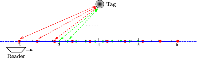
Example of a reader moving along a linear trajectory on the x axis to localize a tag in p = [4,1]; N = 10 phase samples between x = 2 m and x = 6 m (red) or between x = 3 m and x = 5 m (green)
Fig. 5 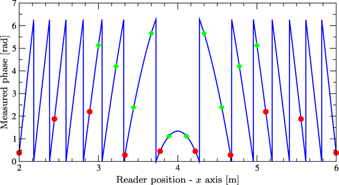
Measured phase for the scenario of Fig. 4 (f = 868 MHz, λ = 35 cm)
-
2.
It affects the localization accuracy due to the relative position between the reader and the tag. This effect is usually known as geometric dilution of precision (GDOP), and it is intrinsic of every localization system [8].


Moreover, it can be noticed how the phase behavior changes with the readers’ position. In fact, when the reader is far from the tag we have (x−xTi)2≫(y−yTi)2, and the relation between the measured phase and the reader’s position on the x axis is almost linear (without considering the [0÷2π] representation), that is \({\phi _{i}({\textbf {p}})\approx -\frac {4\pi f_{i}}{c} \left (x-{x_{\mathrm {T}i}}\right)}\). In this region, we observe a 2π jump of the measured phase approximately every λ/2. Differently, when the reader approaches the tag, by moving along a different direction, the non-linear relation between the measured phase and the reader’s position along the x axis can be seen in Fig. 5.
The next section will derive the ML estimator for determining the tag position, that is, the scheme to process the collected phase data.
3 Phase-based localization
Now, the ML estimator for the position of the tag, adopting phase measurements taken by the reader, is derived.
The likelihood function of the ith observation given p and ai is [35]
where ℜ(·) stands for the real part of a complex number and (·)∗ indicates the conjugate. The likelihood function independent of ai can be obtained by plugging an estimate \(\widehat {a}_{i}\) of ai into (9) [9], that is
By adopting the ML criterion, it is
This can be explicitly computed according to
so that it is obtained \(\widehat {a}_{i}=\tilde {a}_{i}\cos {(\varphi _{i}-\phi _{i}({\textbf {p}}))}\), and the likelihood function of the ith observation, now free of nuisance parameters, becomes
Considering multiple observations, thanks to their independence, we have
Then, the maximum likelihood estimate \({\widehat {\textbf {p}}}\) of the tag position p is
As usually assumed, the position can be determined with the discretization of the search space in a grid approach [19], then testing all the possible hypotheses for p, and taking the most probable. In practice, the sequence of measured phase values (6) is properly correlated using (14) with a hypothetical sequence (7) according to the position p under testFootnote 5.
Notice that, according to (14), each phase measurement is weighted by the received power \(\tilde {a}_{i}^{2}\) returned by the reader. In this manner, the phase values related to higher SNR have a greater impact on the overall likelihood function and contribute heavily to the position estimation.
3.1 Special case: constant amplitudes
The estimator previously derived exploits the measurements of both phase and amplitude taken on the received signal. If an estimator structure resorting to phase measurements only wants to be obtained, as often considered in the literature, a simplified model assuming constant amplitude of the received signal can be considered. In this case, we can neglect the presence of the ai from (7) assuming
Then, we have
and the maximum likelihood estimate \({\widehat {\textbf {p}}}\) of the tag position p is
where the approximation holds at high SNR.
Notice that, using the ML approach with different signal models, we have obtained a sort of maximal ratio combining (MRC) estimators (through (14) and (16)) or equal gain combining (EGC) estimator (through (17)). The corresponding performance will be presented in Section 5.
4 Other approaches
For comparison purposes, in this paragraph, the obtained ML estimator structure is compared with other approaches already proposed in the literature.
In [19], the position is obtained as
In Section 5 the performance of this estimator will be compared with (14) and (16), since it resorts to both amplitude and phase. Moreover, in order to obtain an estimator exploiting phase-only measurements, (18) was also proposed by posing \(\tilde {a}_{i}=1, \forall i\). Such estimator, not accounting for the amplitude of the signal, will be compared with (17).
Differently, [14] proposed to consider phase-difference values. In particular, the following expression is adopted
where (·)H denotes the Hermitian operator (conjugate transpose) and a(p), y are phase-difference vectors obtained as difference between the generic phase value and the first measure. Specifically, they are defined as [14]
Since ∥a(p)∥2=∥y∥2=N, by making explicit the vector product, (19) corresponds to
Equivalently, (22) can be written as
Then, it has been proved that the approach (19), resorting to phase differences reported in (20) and (21), is formally equivalent to (18) with constant amplitudes, then presenting the same performance. In fact, phase is relative because of its periodic behavior, so considering phase differences with respect to a fixed reference (i.e., the first measurement) shall not improve or degrade the performance.
5 Results and discussion
In this section, the performance of the derived ML estimators is compared with that of the approaches already proposed in the literature.
5.1 Numerical setup
We consider a single-antenna reader moving along a rectilinear trajectory on the x axis and taking N = 10 equally spaced measurements between x = 3 m and x = 5 m, with y = 0 m. The tag to be localized is located in p =[5,1].
A single-channel CW signal is considered for all the interrogations, with frequency fi = 868 MHz, ∀i. Signal amplitude of each sample is simulated according to the two-way path loss in free space. The SNR is defined as average among the different samples constituting the observation vector.
For what concerns the implementation of the algorithms for position estimation, a 1D search along the x axis is considered, by assuming known the tag coordinate y = 1. The search for the tag position along the x axis is performed between x = 2 m and x = 8 m, with step 1 mm.
Results are presented in terms of root-mean-square error (RMSE) of the tag position estimation obtained among all the Monte-Carlo trials. Specifically, 105 trials were considered in the simulations.
5.2 Variable amplitude
Figure 6 reports the RMSE of the tag position estimation as a function of the SNR, for different estimators. In particular, the results obtained with the ML estimators are reported, together with the results for approach (18), for both amplitude and phase or phase-only (i.e., (19)/(23)). In order to easy the reading of the figures, the legends report the equation related to a specific approach together with indication MRC for estimators (14), (16), and (18), which use the received signal amplitude to weight the phase terms, or with indication EGC for estimators (17) and (23) exploiting only the phase information.

Localization RMSE as a function of the SNR for various estimator structures; variable amplitude. Continuous lines refer to the ML estimators here proposed. Dashed lines refer to other approaches from the literature
As it is possible to notice, at high SNR all the ML estimators outperform the approaches proposed in the literature, regardless the adoption of phase-only (i.e., (18)) or both amplitude and phase (i.e., (23)). Figure 6 shows that (14) ensures the best performance in the asymptotic region. Similar performance is given by (16); in this case, the small degradation is due to the model mismatch, since the latter was derived from the assumption of constant amplitude signal, which does not correspond to the simulated scenario. A small performance degradation is offered by estimator (17), which does not require the availability of the signal amplitude then leading to a simpler implementation. At high SNR, 3 dB of performance gap is present between (14) (i.e., the MRC approach) and (17) (i.e., the EGC approach).
Comparison between ML estimators and other approaches presented in [14, 19] shows the enhanced performance of the first group. In particular, if we consider the asymptotic region, an error of 10−3 m can be obtained with 20 dB SNR for (14), and 35 dB SNR for (18) (not displayed for space constraints), resulting in a 15 dB gap. Similarly, at 20 dB SNR, the difference between the two approaches is of about 5 times on the achievable RMSE.
In general, it is possible to notice the classical behavior of non-linear estimators, with different operating regions at different SNR [34, 35]. At low SNR, the performance becomes quickly quite poor for all the estimators. In this region, approach (18) has a performance slightly improved with respect to the ML estimators. The explanation of such a phenomenon can be found in the structure of the functions that are maximized. Figure 7a shows the likelihood function (14), in the absence of measurement noise. Differently, the function (18) is depicted in Fig. 7b. It is possible to notice the sharpness of the main lobe of (14), for which the ML is expected to work very well in the high SNR region, where the probability of selecting the correct lobe is high.Footnote 6 Differently, the performance of (18) in this region is intrinsically poorer, due to the larger main lobe. The situation swaps at low SNR, where the noise could lead to ambiguities in the selection of the main lobe of (14); in this case a smoother behavior, as reported in Fig. 7b, could be beneficial.
5.3 Constant amplitude
With Fig. 6, it has been shown that the performance of the estimator exploiting phase-only (i.e., EGC) is poorer due to the mismatch with the signal model. For comparison purposes, in Fig. 8 the RMSE of the tag position estimation as a function of the SNR is reported in the case of constant amplitude for the received signal, that is, without accounting of the path loss in the simulation. Again, it is possible to appreciate the increased accuracy offered by the ML (16) with respect to approach (18) and (23). Moreover, approximation (17) is showed to hold, especially in the asymptotic region, thanks to the supposed constant amplitude in the model adopted. In this case, estimators accounting for variable amplitude show a degraded performance due to the model mismatch, so that the use of the phase information only is beneficial, especially at medium SNR, due to the absence of any variation in the amplitude of the received signal (ideal case). It is interesting to see that the presence of a signal with constant amplitude for all the samples does not improve significantly the estimation accuracy which can be obtained in the asymptotic region, but moves significantly the SNR value where such a region starts. In fact, for the ML estimator (16), the asymptotic region starts at 9 dB SNR in case of signal with constant amplitude, while 16 dB SNR are necessary in case the signal path-loss for every phase sample is considered in the simulation.

Localization RMSE as a function of the SNR for various estimator structures; constant amplitude. Dashed lines refer to other approaches from the literature
5.4 Effects of the tag position
Previous results presented the performance of the different estimators for a tag placed in a specific position. However, it is well known that, in localization problems, the performance changes depending on the relative positions of readers and tags, since both measurements’ quality and the geometric configuration (i.e., GDOP) play a crucial role [8, 36], as briefly discussed in Section 2.3. In order to show how the tag position impacts its position estimation capability with phase-based techniques, Fig. 9 presents the RMSE in this setting. In particular, the ML (16) and (18) are considered.

Localization RMSE as a function of the tag position along the x axis, for various estimator structures
It is possible to notice that the derived ML outperforms the other approach for every tag position at the selected SNR of 15 dB. Depending on the tag position, up to one order of magnitude of difference in the localization accuracy is experienced (e.g., for x = 2 m or x = 6 m). Differently, when the tag is located along the direction orthogonal to the middle point of the synthetic aperture described by the reader, the two approaches presents the same performance. Notice that uniform spatial samples along the synthetic aperture where considered in the simulation.
6 Conclusion
This paper presented the structure of the ML estimator for the position of a RFID tag, using phase measurements. The derivation was conducted under different models of the received signal, in order to obtain estimators exploiting only the phase information, or both amplitude and phase. The derived estimators were compared with the approaches already proposed in the literature, showing the performance improvement that can be obtained using the proposed signal processing scheme. Moreover, it has been proved that other approaches presented in the literature lead to the same estimation structure, then presenting equivalent performance.
It has been shown how approaches that properly weights the phase information with the received signal amplitude ensure the best performance. In the high SNR regime, the use of the ML estimator corresponds to an improvement of up to one order of magnitude in the estimation error for certain tag positions. Differently, at low SNR the performance of all the estimators is similar and ambiguities limit severely the effectiveness of these positioning schemes.
Future research attention should be devoted in determining the design criteria of these positioning schemes, since many aspects affect the feasibility of the localization and the performance, as the number of measurements and their position (i.e., the spatial sampling), frequency, tag position, and number of antennas. Finally, the characterization of the effects of multipath propagation, which can severely affect the phase information, should be investigated, also considering experimental studies in real scenarios.
Notes
Additional phase shifts due to the circuits at reader and tag side [13] are supposed calibrated out.
Notice that, according to the approaches proposed in the following, ambiguity is not resolved explicitly as in other approaches [39], but every new measurement poses additional constraints to the problem, then making feasible the position estimation.
Fig. 2 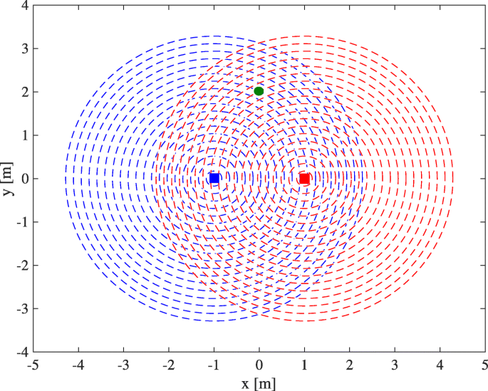
Example of geometric configuration for the phase-based localization of a passive tag (f = 868 MHz, λ = 35 cm): two readers are considered in coordinates [−1, 0] (blue) and [1, 0] (red); a tag is considered in [0, 2] (green). Intersections of circles denote the possible locations of the tag considering the two phase measurements (first 20 displayed)
Notation si(p,ai) denotes that the sample si is a function of the tag position p, to be estimated, and of the unknown parameter ai.


References
K. Finkenzeller, RFID Handbook: Fundamentals and Applications in Contactless Smart Cards and Identification, 3rd ed. (Wiley, 2010).
EPCGlobal, Class 1 generation 2 UHF air interface protocol standard v.1.0.9. (2005).
A. Costanzo, D. Masotti, T. Ussmueller, R. Weigel, Tag, you’re it: ranging and finding via RFID technology. IEEE Microw. Mag. 14(5), 36–46 (2013).
R. Miesen, R. Ebelt, F. Kirsch, T. Schafer, G. Li, H. Wang, M. Vossiek, Where is the tag?. IEEE Microw. Mag. 12(7), 49–63 (2011).
L. M. Ni, D. Zhang, M. R. Souryal, RFID-based localization and tracking technologies. IEEE Wirel. Commun. 18(2), 45–51 (2011).
H. Wymeersch, J. Lien, M. Z. Win, Cooperative localization in wireless networks. Proc. IEEE. 97(2), 427–450 (2009).
B. Etzlinger, F. Meyer, F. Hlawatsch, A. Springer, H. Wymeersch, Cooperative simultaneous localization and synchronization in mobile agent networks. IEEE Trans. Signal Process. 65(14), 3587–3602 (2017).
D. Dardari, E. Falletti, M. Luise, Satellite and terrestrial radio positioning techniques - a signal processing perspective (Elsevier Ltd, London, 2011).
C. W. Helstrom, Statistical theory of signal detection, 2nd ed. (Oxford: Pergamon Press, Headington Hill Hall, 1968).
D. Dardari, A. Conti, U. Ferner, A. Giorgetti, M. Win, Ranging with ultrawide bandwidth signals in multipath environments. Proc. IEEE. 97(2), 404–426 (2009).
N. Decarli, F. Guidi, D. Dardari, Passive UWB RFID for tag localization: architectures and design. IEEE Sensors J. 16(5), 1385–1397 (2016).
D. Dardari, N. Decarli, A. Guerra, F. Guidi, in IEEE Int. Conf. on RFID. The future of ultra-wideband localization in RFID, (2016), pp. 1–7.
P. V. Nikitin, R. Martinez, S. Ramamurthy, H. Leland, G. Spiess, K. V. S. Rao, in IEEE Int. Conf. RFID. Phase based spatial identification of UHF RFID tags, (2010), pp. 102–109.
A. Buffi, P. Nepa, F. Lombardini, A phase-based technique for localization of UHF-RFID tags moving on a conveyor belt: performance analysis and test-case measurements. IEEE Sensors J. 15(1), 387–396 (2015).
A. Buffi, M. R. Pino, P. Nepa, Experimental validation of a SAR-based RFID localization technique exploiting an automated handling system. IEEE Antennas Wirel. Propag. Lett. PP(99), 11–1 (2017). early access online.
M. Wegener, D. Fro, M. Rler, C. Drechsler, C. Ptz, U. Heinkel, in Int. Multi-conference on systems, signals devices. Relative localisation of passive UHF-tags by phase tracking, (2016), pp. 503–506.
M. Vossiek, A. Urban, S. Max, P. Gulden, Inverse synthetic aperture secondary radar concept for precise wireless positioning. IEEE Trans. Microw. Theory Tech. 55(11), 2447–2453 (2007).
R. Miesen, F. Kirsch, M. Vossiek, in IEEE Int. Conf. RFID. Holographic localization of passive UHF RFID transponders, (2011), pp. 32–37.
R. Miesen, F. Kirsch, M. Vossiek, UHF RFID localization based on synthetic apertures. IEEE Trans. Autom. Sci. Eng. 10(3), 807–815 (2013).
R. Zhao, Q. Zhang, D. Li, H. Chen, D. Wang, in Int. symp. world of wireless, mobile and multimedia networks. A novel accurate synthetic aperture RFID localization method with high radial accuracy, (2017), pp. 1–9.
L. Shangguan, Z. Yang, A. X. Liu, Z. Zhou, Y. Liu, STPP: Spatial-temporal phase profiling-based method for relative RFID tag localization. IEEE/ACM Trans. Networking. 25(1), 596–609 (2017).
X. Fu, A. Pedross-Engel, D. Arnitz, M. S. Reynolds, in IEEE SENSORS. Simultaneous sensor localization via synthetic aperture radar (SAR) imaging, (2016), pp. 1–3.
E. DiGiampaolo, F. Martinelli, Mobile robot localization using the phase of passive UHF RFID signals. IEEE Trans. Ind. Electron. 61(1), 365–376 (2014).
M. Scherhufl, M. Pichler, A. Stelzer, UHF RFID localization based on phase evaluation of passive tag arrays. IEEE Trans. Instrum. Meas. 64(4), 913–922 (2015).
M. Scherhufl, M. Pichler, A. Stelzer, UHF RFID localization based on evaluation of backscattered tag signals. IEEE Trans. Instrum. Meas. 64(11), 2889–2899 (2015).
S. Sarkka, V. V. Viikari, M. Huusko, K. Jaakkola, Phase-based UHF RFID tracking with nonlinear kalman filtering and smoothing. IEEE Sensors J. 12(5), 904–910 (2012).
C. Zhou, J. D. Griffin, Accurate phase-based ranging measurements for backscatter RFID tags. IEEE Antennas Wirel. Propag. Lett. 11:, 152–155 (2012).
L. Shangguan, Z. Yang, A. X. Liu, Z. Zhou, Y. Liu, in 12th USENIX Symposium on networked systems design and implementation (NSDI 15). Relative localization of RFID tags using spatial-temporal phase profiling (USENIX AssociationOakland, CA, 2015), pp. 251–263.
L. Shangguan, Z. Li, Z. Yang, M. Li, Y. Liu, J. Han, OTrack: Towards order tracking for tags in mobile RFID system. IEEE Trans. Parallel Distrib. Syst. 25(8), 2114–2125 (2013).
S. Bartoletti, N. Decarli, A. Guerra, F. Guidi, D. Dardari, A. Conti, Order of arrival estimation via UHF-UWB RFID (IEEE International Conference on Communications Workshops (ICC), Sydney, 2014).
A. Buffi, P. Nepa, The SARFID technique for discriminating tagged items moving through a UHF-RFID gate. IEEE Sensors J. 17(9), 2863–2870 (2017).
J. Wang, D. Katabi, in Proceedings of the ACM SIGCOMM 2013 conference. Dude, where’s my card?: RFID positioning that works with multipath and non-line of sight (ACMNew York, 2013), pp. 51–62.
J. Liu, F. Zhu, Y. Wang, X. Wang, Q. Pan, L. Chen, in Proc. of the IEEE conf. on computer communications. RF-scanner: Shelf scanning with robot-assisted RFID systems, (2017), pp. 1–9.
H. L. V. Trees, Detection, Estimation, and Modulation Theory: Part I, 2nd ed. (Wiley, New York, 2001).
S. M. Kay, Fundamentals of statistical processing: estimation theory (Prentice-Hall Signal Processing Series, 1993). vol. 1.
Y. Shen, M. Z. Win, Fundamental limits of wideband localization – Part I: a general framework. IEEE Trans. Inf. Theory. 56(10), 4956–4980 (2010).
J. Kimionis, A. Bletsas, J. N. Sahalos, Increased range bistatic scatter radio. IEEE Trans. Commun. 62(3), 1091–1104 (2014).
N. Decarli, F. Guidi, D. Dardari, A novel joint RFID and radar sensor network for passive localization: design and performance bounds. IEEE Sel. J. Topics Signal Process. 8(1), 80–95 (2014).
S. Schwarzer, M. Vossiek, M. Pichler, A. Stelzer, in IEEE Radio and Wireless Symposium. Precise distance measurement with IEEE 802.15.4 (zigbee) devices, (2008), pp. 779–782.
Acknowledgements
The author would like to thank F. Guidi for the fruitful discussions and carefully reading the manuscript, and the anonymous reviewers for the constructive comments provided.
Funding
This research has been supported, in part, by the European Space Agency project LOST and by the EU Horizon 2020 research and innovation programme under the project XCycle (grant no. 635975).
Availability of data and materials
Not applicable.
Author information
Authors and Affiliations
Contributions
The author read and approved the final manuscript.
Corresponding author
Ethics declarations
Competing interests
The author declares that he has no competing interests.
Publisher’s Note
Springer Nature remains neutral with regard to jurisdictional claims in published maps and institutional affiliations.
Rights and permissions
Open Access This article is distributed under the terms of the Creative Commons Attribution 4.0 International License (http://creativecommons.org/licenses/by/4.0/), which permits unrestricted use, distribution, and reproduction in any medium, provided you give appropriate credit to the original author(s) and the source, provide a link to the Creative Commons license, and indicate if changes were made.
About this article

Cite this article
Decarli, N. On phase-based localization with narrowband backscatter signals. EURASIP J. Adv. Signal Process. 2018, 70 (2018). https://doi.org/10.1186/s13634-018-0590-4
Received:
Accepted:
Published:
DOI: https://doi.org/10.1186/s13634-018-0590-4