
Abstract
The complexity of agent localization increases significantly when unique identification of the agents is not possible. Corresponding application cases include multiple-source localization, in which the agents do not have identification sequences at all, and scenarios in which it is infeasible to send sufficiently long identification sequences, e.g., for highly resource-limited agents. The complexity increase is due to the need to solve an additional optimization problem to resolve the indifferentiability of the agents and thus to enable their localization. In this work, we present a thorough analysis of this problem and propose a maximum a posteriori (MAP)-optimal algorithm based on graph decompositions and expression trees. The proposed algorithm efficiently exploits the fixed-parameter tractability of the underlying graph-theoretical problem and employs dynamic programming and backtracking. We show that the proposed algorithm is able to reduce the run time by up to 88.3% compared with a corresponding MAP-optimal integer linear programming formulation.
1 Introduction
The unique identification of wireless sensors or agents is generally regarded as an axiomatic design criterion for wireless systems. However, in certain application cases, unique identification is either inherently impossible, such as in multiple-source localization, or infeasible because of application-specific constraints. In many scenarios, agent localization relies on pairwise inter-sensor distance measurements, for which precise information about the identification of the agents and the obtained measurements is required when using classical localization algorithms. In cases in which unique identification is not possible, the localization of wireless agents requires solving an additional optimization problem to overcome the non-unique identification of the agents. In this work, the corresponding problem is thoroughly analyzed and an efficient and optimal algorithm is presented. Subsequently, a relevant use case for these algorithms is presented.
An upcoming application case for wireless sensors in which non-unique identification will play a key role is the exploration of environments that are accessible only by miniature sensorsFootnote 1. Such environments include groundwater systems and, as considered in [1], hardly permeable cold heavy oil production with sand (CHOPS) mining areas. In both cases, the idea is to utilize wireless sensors to explore the environment and gather information regarding, e.g., the structure of the underground system, the physical properties of the sensor-carrying fluid, and the general resource richness. For these scenarios, the sensor motes need to satisfy the following requirements, which are mainly derived from or mentioned in [1]:
-
An outer diameter of less than 5 mm to ensure that a significant number of the sensors remain intact after passing through the injection pumps.
-
A robust shell able to withstand pressures of up to 6 MPa [2].
-
Several tens of thousands of sensor motes to survey a significant portion of the environment while accounting for the fact that many sensors will be destroyed and remain unrecovered in the environment. In this regard, [1] report an extraction ratio of approximately 8%. The large required number of agents is also motivated by the limited sensing range of each agent.
-
Energy supply for an operating time of approximately 48 h.
To facilitate the localization of the agents, they are equipped with ultrasonic transceivers and perform ranging by measuring the round-trip times to other agents. These measurements are only stored locally and are not forwarded to nearby agents. The positioning, i.e., localization, of the sensor motes is performed offline after the extraction of the agents by a central unit, which can utilize significant computational resources for this purpose. This unit has access to all measurements recorded by the recovered agents.
In this scenario, the following conditions lead to the conclusion that unique identification of the agents is not feasible:
-
1.
The small sensor size and the long operation time significantly constrain the consumable energy, particularly because the majority of the available space inside the agents is already occupied by hardware such as transceivers and environmental sensors.
-
2.
Because of the small sensor mote size and its implications, Direct-Sequence (Spread Spectrum) Code-Division Multiple Access (DS-CDMA) approaches are needed because, e.g., frequency-division multiple access (FDMA) and TDMA require both a wide bandwidth and sharp filtersFootnote 2 and accurate synchronization, respectively, and thus cannot be used. For DS-CDMA, it is known that the code length is equal to the number of users in the networkFootnote 3. Thus, the use of unique codes would result in excessive power consumption for the transmission of each ranging pulse.
Consequently, only shorter—meaning non-unique—DS-CDMA codes can provide a reduction in the energy requirements that is sufficient to enable this application scenarioFootnote 4. Therefore, the central unit (fusion center) needs to resolve the resulting ambiguities in the pairwise distance measurements, before positioning using classical localization algorithms will be possible.
It is believed that a computationally intensive tracking of the agents can be replaced by several quasi-static localizations whenever the swarm is distributed entirely within the environment. This is because on the one hand many agents are needed for the exploration and because on the other hand it may take long for the agents to pass through the environment. Consequently, a further important task is to estimate—based on the agent measurements—when these localizations should take place.
Note that the underlying problem of insufficient time or frequency resources to uniquely address all agents can likewise occur in other multiple-access schemes. Additionally, note that there is no negative impact regarding, e.g., the signal processing, hardware resources, or energy consumptions of the agents as a result of the non-unique identification. This is because the increased localization complexity that results from non-unique identification and the resolution of the resulting ambiguities are borne by the fusion center.
In this work, the implications of non-unique identification for the localization of sensor motes are investigated. In this regard, we show that non-unique identification results in an additional optimization problem beyond the actual localization itself. We refer to this additional problem as the transmit-ambiguity resolution problem (TARP). To address this problem, we propose an algorithm that is able to resolve the ambiguities optimally in the sense of the maximum a posteriori (MAP) probability and that is up to 8.55 times faster than an equivalent integer linear programming (ILP) formulation, which is \(\mathcal {NP}\)-hard in general and which serves as a baseline in this work. This corresponds to a run-time reduction of 88.5%. The algorithms presented in this work are designed to be used in conjunction with classical localization algorithms, such as those based on semidefinite programming [3–9], second-order cone programming (SOCP) [10], or least-squares methods [11, 12], for the described scenarios. Consequently, it is said that the presented algorithms re-enable the localization with existing localization algorithms.
1.1 Related work
Motivated by an initial feasibility study regarding the exploration of inaccessible environments [1] and related experiments in which the need for shared transmission identifiers has been foreseen, the authors of [13] presented the first procedure aimed at resolving the transmit ambiguities caused by non-unique identification for FDMA-based scenarios. The presented method was heuristic and was not derived from an optimality measure such as minimum mean-squared error (MMSE) or maximum-likelihood (ML). Moreover, its complexity was not analyzed, and measurement noise was not explicitly considered. The proposed method relied on a neighbor-matching procedure in which the ambiguities were resolved by comparing the distance measurements of neighboring sensors.
In [14], we extended this approach to purely additive noise scenarios using adjacency and neighborhood estimation. In [15], we considered a joint localization and transmit-ambiguity resolution approach in which a heuristic was used to resolve the ambiguities.
Moreover, in our conference work [16], we introduced the concept of dynamic programming on k-ambiguity trees by exploiting fixed-parameter tractability to efficiently solve the TARP. The run time of this method was compared with that of the integer programming implementation of the MMSE-optimal algorithm.
1.2 Contributions
The contribution of this work is fourfold: First, we present a detailed and comprehensive mathematical formulation of the TARP, which arises in the case of the non-unique identification of sensor motes, including the governing equations and its optimal ILP-based optimization problem. Second, we propose to use dynamic programming instead of solving the \(\mathcal {NP}\)-hard ILP problem to re-enable the localization of the agents. Third, we describe a new representation of the problem using k-ambiguity trees, which are derived from k-expression trees and are used in a dynamic programming manner to solve the problem optimally. This tree representation is based on a fixed-parameter tractability analysis, which is the basis for the efficient solution of the TARP. Fourth, we improve the dynamic programming approach by employing backtracking, which yields a further reduction in the computational complexity by incrementally evaluating partial solution candidates.
Consequently, we propose a methodology that compensates for the inability of these classical methods to address non-relatable distance measurements while maintaining their general applicability for positioning, cf. Fig. 1.

Illustration of the exploration procedure. In step I, agents (visualized in red) are introduced into an unknown environment and perform environmental and distance measurements for mapping and localization, respectively. The agents are carried by the fluid in the environment. Then, the agents are extracted from the environment, and their data are used by a fusion center (step II) to compute the agents’ trajectories (illustrated for two agents). The steps executed by the fusion center for this purpose are as follows: (a) resolve the transmit ambiguities, e.g., with the presented algorithms, and (b) perform positioning using classical localization algorithms. In step III, the environmental measurements and estimated trajectories are used to compute, e.g., the temperature profile of the environment
This work is partly based on our previous conference work [16], which is extended in this work in terms of the following: (1) detailed derivations of the presented algorithms, (2) an extensive evaluation and analysis of the algorithms, and (3) an algorithmic extension via backtracking, resulting in a new dynamic programming methodology.
Moreover, the framework developed in this work can also be extended, for example, to the multiple-source localization problem, which can be regarded as a special case of the problem at hand in which all sources have the same transmit ID.
1.3 Solution overview
This section is dedicated to a less formal description of the problem at hand and the solution steps described in this work. The sensory-agent-based approach for the exploration of unknown environments is depicted in Fig. 1. This figure shows the general procedure, from the introduction of the agents up through their (partial) extraction and the utilization of the agents’ measurements for environmental data reconstruction.
The fusion center, which plays a key role in achieving the goal of obtaining precise information about the underground environment, must address the non-unique identification of the agents and their consequently non-relatable distance measurements. In this regard, the fusion center follows a two-step approach, where the transmit ambiguities are first resolved and then localization is conducted:
-
1.
The resolution of the transmit ambiguities: Conceptually, the purpose of this step is to estimate the proper mapping between the measurements and the agents. In this work, however, a mapping between pairs of measurements and pairs of agents is sought. Such a pair of measurements is called an assignment or solution candidate for the two bidirectional measurements between the corresponding pair of agents. Because of the combinatorial nature of this problem, it is \(\mathcal {NP}\)-hard in general. As shown in Section 3, this problem is related to the independent set problem and can be described as an ILP problem. However, Section 4 motivates the use of dynamic programming to solve this problem more efficiently based on the fact that the problem is fixed-parameter tractable. In this context, it is shown that the clique-width of the graph that describes the resolution problem from a graph-theoretical perspective exerts a significant influence on the solution complexity. For this reason, the following procedure is used in this work to solve the problem:
-
(a)
Based on a thorough analysis of the graph-theoretical problem presented in Section 4, the constraints that govern the combinatorial problem are derived. These constraints are described by vertex sets specifying mutual exclusivity, called constraint cliques in the following.
-
(b)
These constraint cliques, which are the basic entities of the graph-theoretical problem, are used to obtain a tree structure that serves as the basis for computing the complexity-determining clique-width parameter. This computation is performed such that, with a reasonable computational complexity, a complexity parameter k close to the actual clique-width—which is the lowest possible k—is achieved. The corresponding theory and algorithm are introduced in Sections 4 and 5.
-
(c)
Utilizing the previously computed tree structure, dynamic programming methods are used to obtain a solution. The solutions correspond to selected vertices of the vertex sets that specify the mutual exclusivity of the constraint cliques. Consequently, a solution to the combinatorial problem is found, and a mapping between the measurements and the agents is obtained. Two different dynamic programming algorithms are presented in Sections 6 and 7, of which the latter uses a backtracking procedure.
-
(a)
-
2.
The localization of the agents: Based on the mapping between the measurements and the agents, classical localization algorithms can be used for positioning. See, e.g., the last paragraph of Section 1 for an overview of possible solution methods.
1.4 Organization
Based on the steps outlined in Fig. 1, the remainder of this work is structured as follows. In Section 2, the system model and problem formulation are presented. Section 3 introduces the constraints that govern the class of input problems and their graph-theoretical description (Fig. 1, II.a first step). This special graph structure will be exploited in the proposed algorithm to efficiently solve the TARP. Finally, this section presents an overview of the ILP-based problem formulation. Section 4 summarizes the theoretical foundations of the proposed algorithms and introduces the concepts of, e.g., fixed-parameter tractability and expression trees, which are needed for the subsequent discussion of the algorithm design. The proposed algorithms consist of two steps, which are described in Section 5 (Fig. 1, II.a second step) and Section 6 (Fig. 1, II.a third step). Section 5 shows how the graph-theoretical problem can be described using a special variant of the clique-width k-expression tree. In Section 6, this expression tree is used in a dynamic programming algorithm to resolve the transmit ambiguities. An improved backtracking version of this dynamic programming algorithm is described in Section 7 (Fig. 1, II.a third step). A numerical evaluation of the presented methods is presented in Section 8, and Section 9 gives a summary and an outlook regarding future work. To illustrate how the presented algorithms operate, Appendix 1 provides corresponding examples.
2 Problem introduction and system model
In this section, the system model and notation are introduced. Then, a summary of the implications of non-unique identification for agent localization is presented. It is assumed that each sensor has—in addition to its DS-CDMA code, which is henceforth called its ID—a unique serial number (SN) that is only accessible through physical access to the sensors. Such access is possible once the sensors have been extracted from the target environment and centralized localization is being performed. A sensor’s ID, henceforth denoted as \(I_{\mathcal {J}}\) for the Jth ID, is inherently encoded into its ranging pulse, as it serves as the DS-CDMA spreading sequence. The centralized localization unit also knows which IDs are used by which sensors. Hence, the mapping from the SNs to the IDs is known and fixed. The following steps are performed to enable the localization of the sensor motes:
-
1.
The agents, equipped with ultrasonic transducers, are introduced into the environment.
-
2.
The agents record measurements of physical properties such as pressure and temperature. In addition, the agents perform round-trip time (RTT) measurements to facilitate distance estimates to neighboring agents. Because of the strict energy limitations, there is no forwarding or transmission of any data aside from the RTT measurements.
-
3.
The agents are recovered from the environment, and their RTT measurements are jointly processed by the transmit-ambiguity solver to overcome the ambiguities in the distance measurements.
-
4.
Classical localization algorithms are used to estimate the positions of the agents for each time instance when an RTT measurement was made.
The inaccuracy of the RTT ranging procedure is modeled as multiplicative noise. In this model, which has also been adopted by, for example, [7], it is assumed that distance estimates to farther sensors are less accurate. Consequently, the random variable (RV) dj→i, which denotes the distance measured by sensor i based on a ranging pulse sent by sensor j, is given by
where all \(n_{i,j} \sim \mathcal {N}\left (0,\sigma _{i,j}^{2}\right)\) are independently and identically distributed (iid) Gaussian variables with variance \(\sigma _{i,j}^{2}\). Moreover, it is assumed that bidirectional measurements are made. Note that bidirectional communication is also a requirement for RTT measurements. Hence, it is assumed that if sensor i measured a distance to sensor j, then sensor j also measured a similar distance with respect to sensor i. An illustration of the notation is given in Fig. 2. The set of RVs referring to the range measurements received by sensor mote i, which uses ID \(I_{\mathcal {L}}\), from nodes sending with ID \(I_{\mathcal {K}}\) is denoted by \(\mathcal {D}_{i} = \{ d_{j\rightarrow i} \vert j\in \mathcal {K} \}\). The set of distances that sensor i has measured with respect to sensors using \(\mathcal {I}_{K}\) is denoted by \(\mathcal {M}_{i} = \left \{m_{i}^{1},\,m_{i}^{2},\ldots \right \}\), where \({m}_{i}^{l}\) denotes the corresponding lth range measurement of sensor iFootnote 5. As full connectivity is not necessarily given, the following holds: \(\vert \mathcal {M}_{i} \vert \leq \vert \mathcal {D}_{i}\vert \). Consequently, \(\mathcal {M}_{i}\) is an unordered or permuted subset of the random variates, i.e., realizations, of the RVs \(\mathcal {D}_{i}\).
The following definition of the derived problem is used.
Definition 1
[transmit-ambiguity resolution problem (TARP)] The TARP is the problem of overcoming the inability to differentiate among agents that use the same transmit code during communication. In the context of RTT ranging, e.g., for the sake of agent localization, the TARP is the problem of finding the correct mapping between the distance or RTT measurements \(m_{i}^{l}\) and the RVs dj→i and, thus, the agents. Thereby, a decision is made regarding the source of a ranging pulse and its resulting distance or RTT measurement.
An important aspect of the algorithm derivation and the henceforth used notation is that the TARP can be decomposed into independent subproblems, which are given by all pairs of—not necessarily distinct—IDs. In this regard, notice that the ambiguities occurring between two (distinct) groups of agents, each with possibly individual IDs, are not affected by measurements or ambiguities with any other groups of agents. This fact is also illustrated in Fig. 3a. Because of the independence of the subproblems and without loss of generality, only the measurements between sensor motes using, as an example, the IDs \(I_{\mathcal {K}}\) and \(I_{\mathcal {L}}\) are considered in the following.

a Illustration of a network with non-unique identification sequences \(I_{\mathcal {K}}\) and \(I_{\mathcal {L}}\) and their respective distance measurements as seen by the receiving node [14]. The gray arrows and their corresponding measurements are not considered in the subproblem between \(I_{\mathcal {K}}\) and \(I_{\mathcal {L}}\). b Ambiguity corresponding to a, where v5 is given by the pair of measurements indicated in gray between agents “5” and “6.” For clarity, the edges are annotated with the measurements that give rise to them (cf. items 1(a) and 1(b) in the listing in Section 3). Independent of the previous example, c provides a general illustration of how vertices vi,j(l,r) are formed based on the measurement sets \(\mathcal {M}_{i}\) and \(\mathcal {M}_{j}\) of agents i and j, respectively
Example 1
An example of the consequences of the reuse of DS-CDMA codes with respect to localization is illustrated in Fig. 3a. This figure shows two sensor motes, “5” and “6,” that are both using ID \(I_{\mathcal {L}}\). A third sensor mote (“7”) is using ID \(I_{\mathcal {K}}\). Because the sensor motes can differentiate only between different DS-CDMA codes and not between different sensor motes that are using the same code, sensor mote “7” measures two distances that cannot be related to sensor motes “5” and “6.” More precisely, sensor mote “7” measures \(\mathcal {M}_{7} = \left \lbrace m^{1}_{7} m^{2}_{7} \right \rbrace \) (realizations of the RVs contained in \(\mathcal {D}_{7} = \{ d_{5\rightarrow 7}d_{6\rightarrow 7} \}\)), and before offline localization can be performed, the mapping between these measurements and sensors “5” and “6” needs to be estimated.
Consequently, classical localization methods, which do not consider application scenarios with transmit ambiguities—such as [3, 6, 7], which use semidefinite programming, or [11], which uses a linearized least-squares approach—cannot be used without first applying algorithms to resolve the TARP such as those presented in this work.
3 Graph representation and graph problem formulation
In this section, a graph-theoretical formulation of the problem resulting from DS-CDMA code reuse is given. Moreover, a detailed analysis of the problem’s properties, which will be exploited in Section 4, is presented.
The following description utilizes the particular properties of a type of graph whose instances are henceforth called ambiguity graphs. Such a graph is denoted by \(\mathcal {G} = (\mathcal {V},\mathcal {E},\mathcal {W})\), and its components, i.e., the vertex set, edge set and weight function, are defined in the following.
Every vertex of the ambiguity graph is uniquely identified by the notation vi,j(l,r), where i and j refer to agents i and j and l and r refer to their respective lth and rth measurements. Therefore, the vertex vi,j(l,r) refers to the RVs (dj→i,di→j) and their potential realization given by the measurements \(\left (m_{i}^{l},m_{j}^{r} \right)\). In the following, this relation is denoted by \(v_{i,j}(l,r) \overset {\text {ref.}}{\sim } \left (m_{i}^{l},m_{j}^{r} \right)\). Moreover, this vertex has a weight, which corresponds to the likelihood that the measurements \(m_{i}^{l}\) and \(m_{j}^{r}\) were both measured between agents i and j. This section describes how this weight is calculated and presents the definition of the edges of this graph.
Example 2
A simple example of an ambiguity graph for a network is shown in Fig. 3a. For simplicity, a linear index v k is used to denote the vertices of the ambiguity graph. The relationship between this linear notation and the vi,j(l,r) notation is as follows: v1=v5,7(1,1), which relates to \(\left (m_{5}^{1}, m_{7}^{1} \right)\); v2=v5,7(1,2), which relates to \(\left (m_{5}^{1}, m_{7}^{2} \right)\); v3=v6,7(1,1), which relates to \(\left (m_{7}^{1}, m_{6}^{1} \right)\); and v4=v6,7(1,2), which relates to \(\left (m_{6}^{1}, m_{7}^{2} \right)\). With this short-hand notation, the edge and vertex sets for this example are given as follows: \(\mathcal {E}_{1,a}(5,1) = \{(v_{1},v_{2})\}\), \(\mathcal {E}_{1,a}(6,1) = \{(v_{3},v_{4})\}\), \(\mathcal {E}_{1,b}(7,1) = \{(v_{1},v_{3})\}\), \(\mathcal {E}_{1,b}(7,2) = \{(v_{2},v_{4})\}\), \(\mathcal {E}_{2}(5,7) = \{(v_{1},v_{2})\}\), \(\mathcal {E}_{2}(6,7) = \{(v_{3},v_{4})\}\), \(\mathcal {V}_{1,a}(5,1) = \{v_{1},v_{2}\}\), \(\mathcal {V}_{1,a}(6,1) = \{v_{2},v_{4}\}\), \(\mathcal {V}_{1,b}(7,1) = \{v_{1},v_{3}\}\), \(\mathcal {V}_{1,b}(7,2) = \{v_{2},v_{4}\}\), \(\mathcal {V}_{2}(5,7) = \{v_{1},v_{2}\}\), and \(\mathcal {V}_{2}(6,7) = \{v_{3},v_{4}\}\).
The set of edges \(\mathcal {E}\) of the ambiguity graph is the union of three edge sets that satisfy the criteria given below.
-
1.
In the following problem descriptions, edges are used to denote complementary constraints, and any distance measurement \(m_{i}^{l}\) can be assigned to only one RV d∙→i; therefore, edges are introduced as follows:
-
Between \(v_{i,j}(l,r)\overset {\text {ref.}}{\sim } \left (m_{i}^{l},m_{j}^{r} \right)\) and any other vertex \(v_{i,j^{\prime }}(l,r^{\prime }) \overset {\text {ref.}}{\sim } \left (m_{i}^{l},m_{j^{\prime }}^{r^{\prime }} \right)\) that relates to \(m_{i}^{l}\). The set of all edges created based on this condition is denoted by \(\mathcal {E}_{1,a}(i,l)\).
$$ {\selectfont{\begin{aligned} \mathcal{E}_{1,a}(i,l) = \left\{(v_{x},v_{y}) \in \mathcal{V} \times \mathcal{V} \big\vert~ v_{x} \overset{\text{ref.}}{\sim} \left(m_{i}^{l}, m_{j}^{r} \right) \wedge v_{y} \overset{\text{ref.}}{\sim} \left(m_{i}^{l}, m_{j^{\prime}}^{r^{\prime}} \right)\right\} \end{aligned}}} $$(2) -
Between \(v_{i,j}(l,r)\overset {\text {ref.}}{\sim } \left (m_{i}^{l},m_{j}^{r} \right)\) and any other vertex \(v_{i^{\prime },j}(l^{\prime },r) \overset {\text {ref.}}{\sim } \left (m_{i^{\prime }}^{l^{\prime }},m_{j}^{r} \right)\) that relates to \(m_{j}^{r}\). The set of all edges created based on this condition is denoted by \(\mathcal {E}_{1,b}(j,r)\).
$$ {\selectfont{\begin{aligned} \mathcal{E}_{1,b}(j,r) = \left\{(v_{x},v_{y}) \in \mathcal{V} \times \mathcal{V} ~\big\vert~ v_{x} \overset{\text{ref.}}{\sim} \left(m_{i}^{l}, m_{j}^{r} \right) \wedge v_{y} \overset{\text{ref.}}{\sim} \left(m_{i^{\prime}}^{l^{\prime}}, m_{j}^{r} \right) \right\} \end{aligned}}} $$(3)
-
-
2.
Similarly, a pair (tuple) of RVs (dj→i,di→j) can only be matched to at most one tuple of measurements, i.e., one vertex of the ambiguity graph. Therefore, edges are introduced between any vertex vi,j(l,r) and vi,j(l′,r′), i.e., any other vertex that corresponds to the same bidirectional link between sensors i and j. The set of all edges created based on this condition is denoted by \(\mathcal {E}_{2}(i,j)\).
$$ {\selectfont{\begin{aligned} \mathcal{E}_{2}(i,j) = \left\{ (v_{x},v_{y}) \in \mathcal{V} \times \mathcal{V} ~\big\vert~ v_{x} \overset{\text{ref.}}{\sim} \left(m_{i}^{l}, m_{j}^{r} \right) \wedge v_{y} \overset{\text{ref.}}{\sim} \left(m_{i}^{l^{\prime}}, m_{j}^{r^{\prime}} \right) \right\} \end{aligned}}} $$(4)
Consequently, the edge set \(\mathcal {E}\) is given by \(\mathcal {E}~=~\mathcal {E}_{1,a} \cup \mathcal {E}_{1,b} \cup \mathcal {E}_{2} \), where
Note that the index of each edge set, such as 1,a or 2, refers to the corresponding (sub)item and its constraints as given in the listing above.
The objective is to maximize the probability \(\mathbb {P}\) of correctly matching the RVs to the distance measurements given all measurements \(\mathcal {M}_{i}\) from all sensors i, i.e.,
by choosing the weights \(\mathcal {W}(v_{i,j}(l,r))\) of the vertices according to
where \(f_{d_{j\rightarrow i},d_{i\rightarrow j}} (x,y)\) denotes the joint probability density function (PDF) of the RVs dj→i and di→j and, hence, of the noisy distance measurements. A derivation of the PDF used in the numerical evaluation of this work is given in Appendix 2.
Thus, the construction of the ambiguity graph \(\mathcal {G}~=~(\mathcal {V},\mathcal {E},\mathcal {W})\) can be summarized as follows:
-
Every vertex vi,j(l,r) is uniquely identified by a pair of measurements \(\left (m_{i}^{l}, m_{j}^{r} \right)\). This vertex describes a possible solution candidate for the measurement assignment problem. More precisely, it reflects the probability that \(m_{i}^{l}\) and \(m_{j}^{r}\) are the realizations of di→j and dj→i, respectively. In the subsequently described optimization problem, the goal will therefore be to select a subset of these solution candidates.
-
The likelihood that the mapping denoted by vi,j(l,r) is correct is given by the corresponding weight \(\mathcal {W}(v_{i,j}(l,r))\).
-
The edges (cf. Eq. (5)) govern the criteria under which a solution candidate vi,j(l,r) may be selected. Note that the vertices that are subject to particular constraints, such as \(\mathcal {E}_{1,a}(i,l), \mathcal {E}_{1,b}(j,r)\), or \(\mathcal {E}_{2}(i,j)\), are the vertices that are the endpoints of the edges in these sets. The corresponding sets of vertices and their subgraphs are denoted by \(\mathcal {V}_{1,a}(i,l)\), \(\mathcal {V}_{1,b}(j,r)\), and \(\mathcal {V}_{2}(i,j)\) and by \(\mathcal {G}_{1,a}(\cdot,\cdot)~=~\left (\mathcal {V}_{1,a}(\cdot,\cdot), \mathcal {E}_{1,a}(\cdot,\cdot) \right)\), \(\mathcal {G}_{1,b}(\cdot,\cdot)~=~\left (\mathcal {V}_{1,b}(\cdot,\cdot),\mathcal {E}_{1,b}(\cdot,\cdot) \right)\), and \(\mathcal {G}_{2}(\cdot,\cdot)~=~\left (\mathcal {V}_{2}(\cdot,\cdot), \mathcal {E}_{2}(\cdot,\cdot) \right)\).
-
Every vertex \(v_{i,j}(l,r) \overset {\text {ref.}}{\sim } \left (m_{i}^{l}, m_{j}^{r} \right)\) is part of the three subgraphs \(\mathcal {G}_{1,a}(i,l)\), \(\mathcal {G}_{1,b}(j,r)\), and \(\mathcal {G}_{2}(i,j)\). This is because by the definition of item 1(a) in the listing above, vi,j(l,r) is adjacent to any other vertex that relates to the measurement \(m_{i}^{l}\), and by the definition of item 1(b), vi,j(l,r) is also adjacent to any other vertex that relates to the measurement \(m_{j}^{r}\). Moreover, vi,j(l,r) is a solution candidate for the measurements between agents i and j and hence is also an endpoint of the edges in \(\mathcal {E}_{2}(i,j)\) and is therefore adjacent to the vertices in \(\mathcal {V}_{2}(i,j)\).
For brevity and simplicity, in the following, we may refer to the vertices vi,j(l,r) as v k , \(k\in \{1,\ldots,\vert \mathcal {V}\vert \}\), if the additional information provided by the indices i, j, l, and r of vi,j(l,r) is not relevant.
Based on the definition of the ambiguity graph given above, it is easy to verify that the optimal resolution of the transmitter ambiguities, in the sense of maximizing (6) for all assignments \(\left (m_{i}^{l}, m_{j}^{r}\right)\), is equivalent to solving the following minimum-weight independent set problem with size constraints (MW-ISP-SC):
where x k is either one or zero and indicates whether vertex k of the ambiguity graph is in the solution set or not, respectively. This means that any measurements \( \left (m_{i}^{l}, m_{j}^{r} \right)\) that are in the solution set, i.e., whose corresponding vertices vi,j(l,r) are in the independent set, are chosen as the realizations of the RVs (dj→i,di→j). Furthermore, w k denotes the weight of vertex \(v_{k} \in \mathcal {V}\), i.e., \(w_{k}~=~\mathcal {W}(v_{k})\). Constraint (8e) ensures the independence of the set by allowing at most one of two adjacent vertices to be included in the solution set. Constraints (8b) to (8d) refer to the conditions described in items 1(a), 1(b), and 2 of the listing above and constitute additional constraints compared with the classical independent set problem; they are called size constraints because they enforce independent sets of a particular size.
Note that because of the choice of the vertex weights (cf. Eq. (7)), the solution to Problem (8) corresponds to the feasible solution with the highest probability in the MAP sense (cf. Eq. (6)). In addition, note that Problem (8) is \(\mathcal {NP}\)-hard in general [17, 18].
4 Exploiting the graph structure
Because of the \(\mathcal {NP}\)-hardness of Problem (8), new algorithms are needed that can solve the TARP optimally but more efficiently than regular ILP solvers. Less computationally complex algorithms are particularly necessary to accommodate the large number of agents needed for the considered application case. The idea that serves as the basis for the following sections is to employ dynamic programming to obtain a highly tailored algorithm to facilitate efficient solution generation. This is enabled by exploiting the special graph structure described in Section 3. The underlying principle of this exploitation is the fixed-parameter tractability (FPT) of the problem.
In this regard, Section 4.1 introduces the concept of FPT and a theorem that renders it applicable to the TARP and thereby forms the basis of our chosen dynamic programming approach. Section 4.2 presents an overview of the fundamental graph-theoretical concepts, including graph decomposition, that enable the application of the FPT theorem to the TARP. Based on these concepts, Section 5 introduces a novel variant of this decomposition that is tailored to ambiguity graphs.
4.1 Fixed-parameter tractability
The concept of FPT is generally used to analyze problems and, in particular, to find which parameters significantly influence the computational complexity. This analysis can then be used to design efficient algorithms for solving \(\mathcal {NP}\)-hard problems such as the TARP.
The idea of FPT is to describe the complexity of an \(\mathcal {NP}\)-hard problem as a combination of two aspects: the first depending only on the input, such as the number of vertices of a graph, and the second being given by some fixed parameter of the problem. Generally, a problem is said to be fixed-parameter tractable if some algorithm capable of solving this problem has a complexity of \( \mathcal {O}(\text {poly}(\vert x\vert) f(k)) \), where |x| denotes the size of the input, poly(·) denotes some polynomial function, and f(k) is some arbitrary function of the fixed parameter k [19].
The algorithm proposed in this work is based on a theorem presented by [20], which states that finding the independence number, i.e., the size of the largest independent set, is a fixed-parameter tractable problem in which the complexity parameter k refers to a graph property or parameter known as the clique-width. The clique-width is introduced in detail in Section 4.2 below. Regarding the applicability of this theorem to the TARP, note that in Problem (8), the goal is to find an independent set with a particular independence number that is given by the number of distinct sets of types \(\mathcal {E}_{1,a}(\cdot {},\cdot {})\) and \(\mathcal {E}_{1,b}(\cdot {},\cdot {})\)Footnote 6. Because the decision variant of finding the independence number can be interpreted as answering the question “is there an independent set with a size of at least n?”, the following theorem is applicable to Eq. (8).
Theorem 1
[The problem of finding the independence number is fixed-parameter tractable [20]] The problem of determining the independence number of a graph \(\mathcal {G} = (\mathcal {V},\mathcal {E})\) with a clique-width of at most k has a complexity of \( \mathcal {O}(\vert \mathcal {V} \vert f(k)) \) if \(\mathcal {G}\) is given by a clique-width k-expression.
Consequently, Theorem 1 states that the clique-width k of graph \(\mathcal {G}\) is an important parameter when the desire is to find the independence number of \(\mathcal {G}\). This is highlighted by the fact that for the problem of finding the independence number, [21] specifies the particular function f(k)=2k to concretize the complexity in the FPT theorem above [22]. Consequently, the objective in the following is to find a clique-width k-expression for instances of the ambiguity graph with the minimum possible clique-width k. However, computing the clique-width k of a graph is an \(\mathcal {NP}\)-hard problem in general [23]. Therefore, sub-optimal methods for finding some approximation k′≥k of the clique-width are presented in this work.
To this end, Section 4.2 reviews the concept of the clique-width and shows how graphs can be described by certain operations that yield expressions that can then be modeled using a tree. In this way, a graph is said to be decomposed, e.g., into a tree structure.
Remark 1
The motivation for using tree-structure decompositions of graphs, such as tree-decompositions or clique-width k-expression trees, stems mainly from the fact that the independent set problem, for example, can be efficiently solved by applying dynamic programming on such a representation (tree structure) [20,24]. Our particular interest in decomposing graphs into clique-width k-expression trees is mainly driven by the FPT theorem introduced above and by the fact that the clique-width is upper bounded by the tree-width [25]. Furthermore, note that in our case, in which the decomposition of ambiguity graph instances is desired, the edge set \(\mathcal {E}\) is given by a union of cliquesFootnote 7 (cf. Eq. (5)), which turns out to simplify the formulation of an expression for the clique-width.
4.2 Graph theory definitions and notations: clique-width
Recall that, motivated by Theorem 1, the goal is to find clique-width k-expressions that correspond to ambiguity graph instances to enable efficient algorithms for solving the TARP. To this end, this section reviews the definitions of the clique-width and clique-width k-expression trees; this discussion is mainly based on [20,21].
The clique-width is calculated based on recursive operations on vertex-labeled graphs [20]. These operations construct a new clique-width k-expression tree. In the following, \(\mathcal {G} = (\mathcal {V}_{\mathcal {G}},\mathcal {E}_{\mathcal {G}},{lab}_{\mathcal {G}})\) denotes a k-labeled graph where each vertex label is given by the mapping \({lab}_{\mathcal {G}}: \mathcal {V}_{\mathcal {G}}\rightarrow [\!k]\), with [ k] being the set of natural numbers [ k]:={1,…,k} [21].
Definition 2
[Clique-width [20,21] The clique-width of a graph \(\mathcal {G} = (\mathcal {V},\mathcal {E})\) is the minimum number of vertex labels \({lab}: \mathcal {V} \rightarrow [\!k]\) such that \(\mathcal {G}\) can be constructed by the following operations:
-
Disjoint union of vertex-labeled graphs: Let \(\mathcal {G} = (\mathcal {V}_{\mathcal {G}},\mathcal {E}_{\mathcal {G}},{lab}_{\mathcal {G}})\in {CW}_{k}\) and \(\mathcal {J} = (\mathcal {V}_{\mathcal {J}},\mathcal {E}_{\mathcal {J}},{lab}_{\mathcal {J}})\in {CW}_{k}\) be two vertex-disjoint labeled graphs; then, \(\mathcal {G} \oplus \mathcal {J} := (\mathcal {V}^{\prime },\mathcal {E}^{\prime },lab^{\prime })\) is also in CW k , with \(\mathcal {V}^{\prime } := \mathcal {V}_{\mathcal {G}} \cup \mathcal {V}_{\mathcal {J}}\), \(\mathcal {E}^{\prime } := \mathcal {E}_{\mathcal {G}} \cup \mathcal {E}_{\mathcal {J}}\), and
$$\begin{array}{*{20}l} {lab}^{\prime}(u) := \left\{\begin{array}{ll} {lab}_{\mathcal{G}}(u) & \text{if}\ u \in \mathcal{V}_{\mathcal{G}} \\ {lab}_{\mathcal{J}}(u) & \text{if}\ u \in \mathcal{V}_{\mathcal{J}} \end{array}\right. \end{array} $$ -
Edge introductions \({\eta _{i,j}}: {\eta _{i,j}\left (\mathcal {G} \right)} := (\mathcal {V}_{\mathcal {G}},\mathcal {E^{\prime }}_{\mathcal {G}},{lab}_{\mathcal {G}})\), where
$$\begin{aligned} \mathcal{E}_{\mathcal{G}}^{\prime} :=& \mathcal{E}_{\mathcal{G}} \!\cup\! \big\lbrace\big\lbrace {u,v}\big\rbrace \big| u,v \in \mathcal{V}_{\mathcal{G}}, u \!\neq\! v,\\ {lab}_{\mathcal{G}}(u)\!= &i, {lab}_{\mathcal{G}}(v)\,=\,j \big\rbrace \end{aligned} $$ -
Vertex relabeling \({\rho _{i \rightarrow j}}: {\rho _{i \rightarrow j}\big (\mathcal {G} \big)} := (\mathcal {V}_{\mathcal {G}}, \mathcal {E}_{\mathcal {G}}, {lab^{\prime }}_{\mathcal {G}})\), where
$$\begin{array}{*{20}l} {lab^{\prime}}_{\mathcal{G}}(u) := \left\{\begin{array}{ll} {lab}_{\mathcal{G}}(u) & \text{if}\ {lab}_{\mathcal{G}}\ (u) \neq i\\[-2pt] j & \text{if}\ {lab}_{\mathcal{G}}\ (u) =i \end{array}\right.,\forall u {\in} \mathcal{V}_{\mathcal{G}} \end{array} $$
The resulting expression is called a clique-width k-expression or a CW k -expression.
Using Definition 2, a CW k -tree can also be defined, where the root of the tree corresponds to the original unlabeled ambiguity graph \(\mathcal {G}\). Consequently, at the root r of the expression tree, which corresponds to the complete expression, all vertices must have the same label such that the root of the tree is equal to the unlabeled graph \(\mathcal {G}\).
Table 1 presents examples of CW2-expressions and the corresponding graphs. Note that only k = 2 labels are required to represent \(\mathcal {G}_{6}\), which has four vertices.
Example 3
Figure 4 shows the CW2-tree for the labeled graph \(\mathcal {G}_{6}\) given in Table 1. The vertices of the tree are annotated with the induced subgraphs of the tree nodesFootnote 8. Note that in this example, the original graph, \(\mathcal {G}_{6}\), was already labeled, and hence, the root of the CW k -tree is identical to the original graph, with the same labels.
Generally, the decompositions into CW k -expressions and CW k -trees are not unique, i.e., multiple possible CW k -trees exist for a given graph. The main benefit of representing a graph according to Definition 2 is that the CW k -expression is directly related to the complexity of the MW-ISP-SC, which is of \(\mathcal {O}(\vert \mathcal {V}\vert 2^{k})\).
Moreover, the attempt to solve such a problem using the CW k -tree \(\mathcal {T}\) is motivated by the property that the vertex set of subgraph \(\mathcal {G}_{s}\), which corresponds to tree node s, is partitioned into \(k~\leq ~|\mathcal {V}_{s}|\) sets, as given by the k labels [20]. The reason for this is that during the decomposition of a graph into a CW k -expression tree, the labeling will be performed such that, in the dynamic programming phase, it is sufficient to differentiate between groups of vertices that have different labels.
Example 4
Considering the independent set problem as an example, the independence criterion does not need to be checked for every vertex because all vertices that have the same properties in this regard will have the same label. This is ensured by the design of the labeling function, which is described in the following section. Consequently, for a group of vertices with the same label, a check for independence requires only a single check rather than one check for each vertex in that group.
5 The k-ambiguity tree
To enable the exploitation of the property mentioned in the FPT theorem, i.e., that the clique-width of the input graph is a critical parameter in determining the complexity of the TARP, an algorithm for obtaining the tree description—often called a graph decomposition in the literature, as it disassembles parts of the graph into a tree structure—and related operations are presented in this section. To this end, Section 5.1 introduces a short-hand, tailored version of the operations used in the CW k -expressions. The main difference compared with the CW k operations is from a special design criterion that is subsequently introduced, which leads to the introduction of additional predefined edges. The tree corresponding to this tailored description is called the k-ambiguity tree in the following. Contrary to the notation of the CW k -tree, the leaves of the k-ambiguity tree are chosen to be the subgraphs that correspond to the edge constraint sets \(\mathcal {E}_{1,a}(\cdot,\cdot)\), \(\mathcal {E}_{1,b}(\cdot,\cdot)\), and \(\mathcal {E}_{2}(\cdot,\cdot)\), cf. Eqs. (5a), (5b), and (5c). These subgraphs are denoted by \(\mathcal {G}_{1,a}(\cdot,\cdot) = \left (\mathcal {V}_{1,a}(\cdot,\cdot), \mathcal {E}_{1,a}(\cdot,\cdot) \right)\), \(\mathcal {G}_{1,b}(\cdot,\cdot) = \left (\mathcal {V}_{1,b}(\cdot,\cdot),\mathcal {E}_{1,b}(\cdot,\cdot) \right)\), and \(\mathcal {G}_{2}(\cdot,\cdot) = \left (\mathcal {V}_{2}(\cdot,\cdot), \mathcal {E}_{2}(\cdot,\cdot) \right)\), respectively. Note that according to the definition of the edge constraint sets, they are complete inducedFootnote 9 subgraphs, i.e., cliquesFootnote 10.
Recall, from the definition of CW k -expressions, that any expression with the operators ⊕, ηi,j, or ρi →j, e.g., in the form of \(\mathcal {X}_{1} \oplus \mathcal {X}_{2}\), in the CW k -tree corresponds to the merging of two trees \(\mathcal {T}_{\mathcal {X}_{1}}\) and \(\mathcal {T}_{\mathcal {X}_{2}}\) that, in turn, correspond to the expressions \(\mathcal {X}_{1}\) and \(\mathcal {X}_{2}\), respectively. Consequently, we use \(\mu ({\mathcal {T}_{1}},{\mathcal {T}_{2}})\) to denote a joint operator that applies a sequence of ⊕, ηi,j, or ρi → j operations to serve as a merging operator. This joint operator is motivated by the canonical form of the clique-width expression [26], in which after each disjoint union ⊕, first, several edge introductions ηi,j and then several relabeling operations ρi→j must occur [20].
During this merging process, the key idea is to choose an operation such that its output is an induced subgraph of \(\mathcal {G}\). This is because the number of labels required for induced subgraphs is lower than that for non-induced subgraphsFootnote 11. This merging operation is described in more detail below.

Illustration of a tree node s and its vertex set \(\mathcal {V}_{s}\), which is used to visualize R s (v) for the two vertices vi,j(l,r) and v i ′,j(l′,r). The corresponding vertex sets for vi,j(l,r) are \(\mathcal {V}_{1,a}(i,l)\), \(\mathcal {V}_{1,b}(j,r)\), and \(\mathcal {V}_{2}(i,j)\) and are indicated by dashed contours. The sets \(\mathcal {V}_{1,a}(i',l')\), \(\mathcal {V}_{1,b}(j,r)\), and \(\mathcal {V}_{2}(i',j)\) for v i ′,j(l′,r) are shown with dotted contours. The set \(\mathcal {V}_{1,b}(j,r)\), which is considered for both vertices, therefore has a dash-dotted contour. The purpose of visualizing R s (v) for the two vertices is to check whether all vertices of the abovementioned sets \(\mathcal {V}_{\bullet }(\bullet,\bullet)\) are already included in the vertex set \(\mathcal {V}_{s}\) at the current tree node s. For the two vertices in the example above, we have R s (vi,j(l,r)) = ((0,0),(j,r),(0,0))=R s (v i ′,j(l′,r)) because for both vertices, the corresponding set \(\mathcal {V}_{1,b}(\bullet,\bullet)\) is not fully included in \(\mathcal {V}_{s}\). Consequently, both vertices share the same property, which is captured by R s (vi,j(l,r))=R s (v i ′,j(l′,r)). Therefore, they also have the same label (color)
5.1 The merging operator
The merging operator performs the steps listed below, thereby merging the labeled subgraphs \(\mathcal {G}_{c_{1}(s)}\) and \(\mathcal {G}_{c_{2}(s)}\) to yield the output \(\mathcal {G}_{s}\ =\ (\mathcal {V}_{s},\mathcal {E}_{s},{lab}_{s})\). In the following, we use the index c i (s), i = 1,2, to represent the edge or vertex set of the first or second child of tree node s (see also Fig. 6a).
-
1.
Union of the children’s vertex sets: \(\mathcal {V}_{s}\ =\ \mathcal {V}_{c_{1}(s)} \cup \mathcal {V}_{c_{2}(s)}\).
-
2.
Union of the children’s edge sets and a further edge set \(\mathcal {E}_{c_{1}(s),c_{2}(s)}\): \(\mathcal {E}_{s}\ =\ \mathcal {E}_{c_{1}(s)} \cup \mathcal {E}_{c_{2}(s)} \cup \mathcal {E}_{c_{1}(s),c_{2}(s)}\). The additional edge set \(\mathcal {E}_{c_{1}(s),c_{2}(s)}\) is chosen such that \(\mathcal {G}_{s}\) is an induced subgraph, which—as mentioned above—is the desired criterion for the merging operator. Note that \(\mathcal {G}_{c_{1}(s)}\) and \(\mathcal {G}_{c_{2}(s)}\) are both also induced subgraphs, as they are also the results of merging or are cliques corresponding to leaves of the tree. Therefore, the set \(\mathcal {E}_{c_{1}(s),c_{2}(s)}\) contains only edges of the form \((v_{i},v_{j}), v_{i} \in \mathcal {V}_{c_{1}(s)}, v_{j} \in \mathcal {V}_{c_{2}(s)}\).
-
3.
Vertex relabeling resulting in the fewest possible labels, \(\min _{{lab}_{s}} \vert \big \lbrace {lab}_{s}(v) | v \in \mathcal {V}_{s} \big \rbrace \vert \).
The labeling function required to perform steps 2 and 3 is defined in the following. Recall from Section 3 that every vertex vi,j(l,r) is an element of exactly three cliques, namely, \(\mathcal {G}_{1,a}(i,l)\), \(\mathcal {G}_{1,b}(j,r)\), and \(\mathcal {G}_{2}(i,j)\). Because of this property, all vertices that are adjacent to vi,j(l,r) are in the sets \(\mathcal {V}_{1,a}(i,l)\), \(\mathcal {V}_{1,b}(j,r)\), and \(\mathcal {V}_{2}(i,j)\).
Because the k-ambiguity tree corresponding to the ambiguity graph needs to reflect an increasing number of the properties of the original graph as the considered tree node becomes closer to the root of the tree, and in particular because the root of the tree represents the original graph, a tool is needed for describing which properties of a vertex of the original graph are not currently considered at a given tree node. To this end, a function R s (vi,j(l,r)) is defined that describes the properties of a vertex vi,j(l,r) with respect to its originally adjacent vertices. More precisely, R s (vi,j(l,r)) indicates the membership of the three cliques corresponding to vi,j(l,r) with respect to the subgraph \(\mathcal {G}_{s}\) at tree node s and is defined as follows:

where  is related to the inverted indicator function and is defined as
  if \(\mathcal {V} \subseteq \mathcal {V}_{s}\) and 1 otherwise. Thus, a missing edge to a vertex to which vi,j(l,r) was originally connected is indicated by a non-zero tuple entry. An illustration of this function is provided in Fig. 5.

Examples of k-ambiguity trees. a shows a part of a tree in which the tree nodes consist of the merging operator μ. This visualization is analogous to the general description of clique-width k-expression trees, in which the annotated ambiguity subgraphs \(\mathcal {G}\) are often referred to as bags. b shows the same tree, with the tree nodes—for clarity—replaced by the corresponding labeled ambiguity subgraphs
Considering the labeling of the vertices, every occurring three-tuple value of R s is chosen to correspond to a distinct label in the subgraph of tree node s. Thus, the tuple elements of two vertices, \(R_{c_{1}(s)}(v_{1})\) and \(R_{c_{2}(s)}(v_{2})\), are sufficient to determine whether an edge must be inserted between v1 and v2 by the operator μ (or ηi,j): iff the values and positions of at least one tuple entry in each of \(R_{c_{1}(s)}(v_{1})\) and \(R_{c_{2}(s)}(v_{2})\) are equal and non-zero, then an edge is inserted between v1 and v2. This is because these vertices are part of the same clique in the ambiguity graph, cf. Section 3. Recall that a tuple entry of zero indicates that all edges for the corresponding clique have already been inserted.
Moreover, the function R s determines the relabeling according to the operator μ (or ρi→j). Iff R s (v1)=R s (v2), i.e., if the complete tuples are equal, then v1 and v2 are assigned the same label at s, as illustrated in the following example.
Example 5
We consider two vertices v1 and v2 at tree node s and assume that R s (v1)=((0,0),(1,1), (0,0))=R s (v2). Then, v1 and v2 are both lacking edges to all vertices in clique \(\mathcal {V}_{1,b}(1,1)\) that are not in \(\mathcal {V}_{s}\), i.e., to all \(v\in \mathcal {V}_{1,b}(1,1)\backslash \mathcal {V}_{s}\). Consider the merging of tree node s with another tree node s′ by operator μ: if an edge is inserted between v1 and \(v_{3} \in \mathcal {V}_{s^{\prime }}\), then an edge must also be inserted between v2 and v3 because v1 and v2 have the same properties with respect to their current clique memberships. Therefore, no distinction is needed between vertices v1 and v2 with respect to the edge insertion operation, and consequently, the same label is assigned to both vertices. This label is uniquely determined by R s (v1) = R s (v2).
Note that no two vertices are part of the same three cliques (cf. Section 3), and hence, two vertices can have the same label only if at least one tuple entry of R s is zero for both vertices. At the root r of the ambiguity tree, which corresponds to the entire ambiguity graph \(\mathcal {G}\), all edges are already inserted and \(R_{r}(v_{i}) = ((0,0),\ (0,0),\ (0,0)) \forall v_{i}\in \mathcal {V}\); therefore, only a single label is needed.
5.2 Building the k-ambiguity tree
Using the methods and, in particular, the merging operator defined previously, this section introduces an algorithm that is able to generate k-ambiguity trees based solely on the subgraphs \(\mathcal {G}_{1,a}(\cdot,\cdot)\), \(\mathcal {G}_{1,b}(\cdot,\cdot)\), and \(\mathcal {G}_{2}(\cdot,\cdot)\).
Because finding the clique-width decomposition of a graph \(\mathcal {G}\) is an \(\mathcal {NP}\)-hard problem in general, the decomposition of an ambiguity graph into a k-ambiguity tree can also be efficiently done only in a sub-optimal way. Consequently, only decompositions that require a number of labels greater than the clique-width are of computational interest. However, note that for such a decomposition, there is no need to build the actual ambiguity graph because the equivalent information is also provided by all subgraphs of types \(\mathcal {G}_{1,a}(\cdot,\cdot)\), \(\mathcal {G}_{1,b}(\cdot,\cdot)\), and \(\mathcal {G}_{2}(\cdot,\cdot)\). A subset of these basic entities is therefore chosen as the leaves of the k-ambiguity tree. Note that choosing these cliques as the leaves results in an entry of zero in R s (v) for each vertex \(v\in \mathcal {V}_{s}\). The purpose of this heuristic is to reduce the number of distinct three-tuples at tree nodes closer to the root of the tree and thereby reduce the number of labels.
To simplify the notation in the following steps, \(\mathcal {C}\) is used to denote the set that contains all cliques of types \(\mathcal {G}_{1,a}(\cdot,\cdot)\), \(\mathcal {G}_{1,b}(\cdot,\cdot)\), and \(\mathcal {G}_{2}(\cdot,\cdot)\). Similarly, all labeled cliques are denoted by \(\mathcal {C}_{lab}\).
Example 6
\(\mathcal {G}_{1,a}(i,l)~=~\left (\mathcal {V}_{1,a}(i,l), \mathcal {E}_{1,a}(i,l) \right) \in \mathcal {C}\) and \(\left (\mathcal {V}_{1,a}(i,l), \mathcal {E}_{1,a}(i,l), {lab}_{1,a}(i,l) \right) \in \mathcal {C}_{lab}\).
The set \(\mathcal {T}\) is the set of all partial ambiguity trees, i.e., all possible branches of the ambiguity tree that relate to a certain subgraph of the ambiguity graph \(\mathcal {G}\). Furthermore, the neighborhood \(\mathcal {N}(\mathcal {G}_{i})\) of a labeled subgraph \(\mathcal {G}_{i} = (\mathcal {V}_{i},\mathcal {E}_{i},{lab}_{i})\) consists of those subgraphs \(\mathcal {G}_{j} = (\mathcal {V}_{j},\mathcal {E}_{j},{lab}_{j})\) that have a corresponding element in \(\mathcal {T}\) and are adjacent to each other in the ambiguity graph \(\mathcal {G} = (\mathcal {V}_{\mathcal {G}},\mathcal {E}_{\mathcal {G}})\):
Note that when two subgraphs \(\mathcal {G}_{i}\) and \(\mathcal {G}_{j}\) are merged that are not in each other’s neighborhoods, the merging outcome \(\mu (\mathcal {G}_{i},\mathcal {G}_{j})\) requires lab i +lab j labels. In the opposite case, fewer labels may be required.

The greedy k-ambiguity tree construction algorithm is presented in Algorithm 1. On Line 7, it makes use of the remainder graph \((\mathcal {V}_{\Re }, \mathcal {E}_{\Re },{lab}_{\Re }) = \Re (\mathcal {G}^{\prime },\mathcal {T})\), which has the following properties:
-
It is the labeled induced subgraph with vertices \(\mathcal {V}_{\Re } = \mathcal {V}_{\mathcal {G}^{\prime }} \backslash \mathcal {V}_{\text {in}}\), where \(\mathcal {V}_{\text {in}} \subset \mathcal {V}_{\mathcal {G}^{\prime }}\) is the subset of vertices that already occur in subgraphs corresponding to elements of \(\mathcal {T}\).
-
Because it is an induced subgraph, its edge set is given by the edges in ambiguity graph \(\mathcal {G}\) whose endpoints are both in the vertex set \(\mathcal {V}_{\Re }\) [27].
-
Moreover, \(\Re (\mathcal {G}^{\prime },\mathcal {T})\) is a complete graph, and hence, its edge set can be easily determined.
6 Solving the TARP on the k-ambiguity tree
As shown in Fig. 1, the TARP is solved in two steps, of which the first—i.e., the computation of the k-ambiguity tree—has been presented in the previous section. The second step, in which dynamic programming algorithms are used on the k-ambiguity tree to solve the TARP, is presented in this section.
As mentioned in Section 3, the optimal solution to the TARP corresponds to the solution to the MW-ISP-SC with respect to the ambiguity graph. To solve this problem using dynamic programming on the ambiguity tree, an algorithm similar to the method presented by [20] for determining the independence number of a graph is used. However, two major extensions are made to obtain an algorithm suitable for solving the TARP:
-
1.
Accounting for the weight of an independent set in addition to its size
-
2.
Ensuring feasibility with respect to constraints (8b) to (8d)
In the following, additional notations and concepts are introduced that are needed to describe the dynamic programming algorithm.
The power set of all labels available at a tree node s is denoted by \(\mathcal {P}([\!\kappa (s)])\) and lists all 2κ(s) possible combinations of labels, including the empty set, e.g.,
Moreover,  denotes the set of labels of all vertices in \(\mathcal {V}^{\prime }\subseteq \mathcal {V}_{s}\).
The algorithm proposed hereafter utilizes the following tuple structure. At each tree node s, which corresponds to the subgraph \(\mathcal {G}_{s}~=~(\mathcal {V}_{s},\mathcal {E}_{s},{lab}_{s})\), we define
which is a tuple of length 2κ(s), where each element  , with label set
  , denotes the minimum weight of the MW-ISP-SC such that
  .
.
The corresponding most generic optimization problem for computing the data structure F(s) is given in the following. Note that for consistency with the following sections, the elements of F(s) are denoted by  . The data structures of the children of tree node s are denoted by
  and
and  , cf. Fig. 6a. The elements are given by


where the weights \(\mathcal {W}(v_{i})\) are given by Eq. (7). To enable the recursive computation of F(s),  is obtained as


because the vertex set corresponding to tree node s, \(\mathcal {V}_{s}\), is the union of the vertex sets of the children of s. By the definition of the CW k -tree (cf. Definition 2), for the objective function of Problem (14), it holds that
and for the first constraint of Problem (14), it holds that

where  denotes the label set at tree node s of the vertices labeled with
  at c
i
(s).
at c
i
(s).

In the following, the notation that infeasible sets have a weight of  is adopted. Hence, we regard sets that satisfy
  as solution candidates. Using formulation Eqs. (14), (15), and (16), F(s) will be computed using dynamic programming in a bottom-up fashion, starting from the leaves of the ambiguity tree. The final formulation with additional constraints, which are introduced in the following, is given in Eq. 17 and referenced in Algorithm 2.
6.1 Ensuring the independent set size in the k-ambiguity tree
Constraints (8b) and (8c), which determine the size of the independent set, are equivalent to the requirement that each clique in \(\mathcal {C}_{1,ab}\) must have exactly one vertex in the solution to the independent set problem. The clique set \(\mathcal {C}_{1,ab}\) is defined as a subset of the clique set \(\mathcal {C}\), which was introduced in Section 5.2: \(\mathcal {C}_{1,ab}\) consists of all cliques (complete subgraphs) that are due to ambiguity graph constraints 1(a) and 1(b), i.e., of the \(\mathcal {G}_{1,a}(\cdot,\cdot)\) and \(\mathcal {G}_{1,b}(\cdot,\cdot)\) types. To enable a feasibility check of the size constraint at each tree node s, let \(\mathcal {C}_{1,ab}(s) \subseteq \mathcal {C}_{1,ab}\) denote those cliques whose vertices are completely included in \(\mathcal {V}_{s}\). Now, set  if there is no vertex set \(\mathcal {V}^{\prime }\) with
  that contains a vertex from every clique in \(\mathcal {C}_{1,ab}(s)\).
Example 7
If, e.g., \(R_{c_{1}(s)}(v) = \big ((\alpha _{1},\alpha _{2}), (\beta _{1},\beta _{2}),\) (γ1,γ2)) with α1,α2>0 (cf. Eq. (9)) and R s (v)=((0,0),(β1,β2),(γ1,γ2)), then \(\mathcal {G}_{1,a}(\alpha _{1},\alpha _{2})\) is in \(\mathcal {C}_{1,ab}(s)\), and hence, at tree node s, exactly one vertex \(v \in \mathcal {V}_{1,a}(\alpha _{1},\alpha _{2})\) must be selected as part of the independent set solution. Therefore, it is said that \(\mathcal {G}_{1,a}(\alpha _{1},\alpha _{2})\) imposes a size constraint (SC) at tree node s.
Because each non-leaf tree node s in the k-ambiguity tree is the result of the merging of its two children, i.e., \(\mathcal {G}_{s} = \mu (\mathcal {G}_{c_{1}(s)},\mathcal {G}_{c_{2}(s)})\), the SCs are formulated in terms of the children to enable recursive procedures. This reduces the SC clique set that needs to be checked at parent node s to those cliques that are not included in the constraint clique sets of its children c i (s): \(\mathcal {C}_{1,ab}^{\prime }(s) = \mathcal {C}_{1,ab}(s)\backslash \{ \mathcal {C}_{1,ab}(c_{1}(s)), \mathcal {C}_{1,ab}(c_{2}(s)) \}\).
The dynamic programming procedure operates on the k-ambiguity tree and, therefore, on label sets instead of vertex sets. Hence, the SCs in \(\mathcal {C}_{1,ab}^{\prime }(s)\) must be formulated using label sets. Recall that each label corresponds to a three-tuple of the form given in Eq. (9) and that the first two elements refer to vertex sets of the \(\mathcal {V}_{1,a}(\cdot,\cdot)\) and \(\mathcal {V}_{1,b}(\cdot,\cdot)\) types. If  and
and  correspond to three-tuples \(R_{c_{1}(s)}\) and \(R_{c_{2}(s)}\) that have equal and non-zero entries at the same position, then edges are inserted between vertices with labels of ℓ1 and ℓ2 by the operator μ at tree node s. Therefore, these vertices cannot be part of an independent set and are infeasible. The set of feasible label-set pairs
  at tree node s is denoted by
  .
.
6.2 Dynamic-programming-based algorithm for solving the TARP
A complete algorithmic description of the dynamic programming procedure is given in Algorithm 2Footnote 12. The algorithm is performed in a bottom-up fashion, i.e., starting from the leaves of the k-ambiguity tree. Depending on whether the current tree node is a leaf, F(s) must be computed either from scratch or based on its children c1(s) and c2(s):
-
In the case that s is a leaf, its corresponding subgraph \(\mathcal {G}_{s}\) is an element of clique set \(\mathcal {C}\). If
 addresses more than one vertex, which is not feasible, as indicated by
  . The case in which
  is feasible only for non-SC cliques, i.e., if \(\mathcal {G}_{s}\in \mathcal {C}_{2}\), we set
  .
. -
In the case that s has two children c i (s), i=1,2, the tuple elements of F(s) are computed based on F(c i (s)), i = 1,2, by solving Problem (17). The label set
 is obtained as the union of the relabeled label sets of the children, cf. constraint (17b). Constraint (17c) ensures that the SC is satisfied (cf. Section 6.1), and constraint (17d) ensures that
  is an independent set of ambiguity graph \(\mathcal {G}\). Thus, \(\mathcal {E}_{c_{1}(s),c_{2}(s)}^{lab}\) is the labeled variant of \(\mathcal {E}_{c_{1}(s),c_{2}(s)}\), i.e., it contains the edges that are introduced during the merging of the labels of \(\mathcal {V}_{c_{1}(s)}\) and \(\mathcal {V}_{c_{2}(s)}\).
 addresses more than one vertex, which is not feasible, as indicated by
  . The case in which
  is feasible only for non-SC cliques, i.e., if
  .
. is obtained as the union of the relabeled label sets of the children, cf. constraint (17b). Constraint (17c) ensures that the SC is satisfied (cf. Section
  is an independent set of ambiguity graph


7 Backtracking-based dynamic programming algorithm for solving the TARP
This section introduces a new dynamic programming algorithm that employs backtracking to reduce the number of label-set combinations tested before the optimal solution is found. In this regard, note that in the general formulation of Problem (17), the complete data structure  is computed for every tree node s. However, to solve the TARP and, hence, to compute F(r) for the root r of the tree, only specific elements
  of F(s) from each tree node s are needed. Run-time reductions can be achieved by performing only on-demand computations of the necessary weight elements of the data structure F(s). To this end, bounds \(\beta _{c_{1}(s)}\) and \(\beta _{c_{2}(s)}\) on the lengths of the data structures of the children of tree node s are introduced. The partial data structure is denoted by \(\phantom {\dot {i}\!}F(s,\beta _{s}) = F(s,\beta _{c_{1}(s)},\beta _{c_{2}(s))}\), where β
s
is the bound on the cardinality of F(s,β
s
), which is controlled by the parent nodes of s. Initially, every leaf of the k-ambiguity tree is initialized with a bound of ∞, and all other tree nodes have an initial bound of 1. In general, the bounds will be increased only if additional label-set combinations
of F(s) from each tree node s are needed. Run-time reductions can be achieved by performing only on-demand computations of the necessary weight elements of the data structure F(s). To this end, bounds \(\beta _{c_{1}(s)}\) and \(\beta _{c_{2}(s)}\) on the lengths of the data structures of the children of tree node s are introduced. The partial data structure is denoted by \(\phantom {\dot {i}\!}F(s,\beta _{s}) = F(s,\beta _{c_{1}(s)},\beta _{c_{2}(s))}\), where β
s
is the bound on the cardinality of F(s,β
s
), which is controlled by the parent nodes of s. Initially, every leaf of the k-ambiguity tree is initialized with a bound of ∞, and all other tree nodes have an initial bound of 1. In general, the bounds will be increased only if additional label-set combinations  need to be considered, i.e., if the currently considered combinations—which, by definition, have the lowest possible weight—are infeasible with respect to Problem (17). In general, it is possible to increase the bounds in an arbitrary way. In the following, we let \(\beta _{c_{i}(s)} = f_{\beta }(u_{c_{i}(s)})\) denote the function that determines the new bound, depending on the update counter \(u_{c_{i}(s)}\) of child c
i
(s). This update counter is increased by one whenever a new set of label-set combinations is requested by the parent node.
need to be considered, i.e., if the currently considered combinations—which, by definition, have the lowest possible weight—are infeasible with respect to Problem (17). In general, it is possible to increase the bounds in an arbitrary way. In the following, we let \(\beta _{c_{i}(s)} = f_{\beta }(u_{c_{i}(s)})\) denote the function that determines the new bound, depending on the update counter \(u_{c_{i}(s)}\) of child c
i
(s). This update counter is increased by one whenever a new set of label-set combinations is requested by the parent node.
Recall that each entry  of
of  is the weight of the local MW-ISP-SC at the corresponding tree node, where the solution set only consists of vertices labeled with
  . The bounds \(\beta _{c_{i}(s)}\), i = 1,2, specify the maximum cardinality \(\vert F(s,\beta _{c_{i}(s)}) \vert ~\leq ~ \beta _{c_{i}(s)}\) of the label sets that are considered when computing \(F(s,\beta _{c_{1}(s)},\beta _{c_{2}(s)})\) for the parent tree node s.
The following variables are used to perform the backtracking:
-
anext and bnext denote the next smallest values in F(c1(s)) and F(c2(s)), respectively, that are not currently members of F(c1(s),βc1(s)) and F(c2(s),βc2(s)), respectively.
-
amin and bmin denote the smallest weights in F(c1(s),βc1(s)) and F(c2(s),βc2(s)), respectively.
-
dnext = min{anext + bmin,bnext + amin} is a lower bound on the weight of the next label combinations that are in F(s) = F(s,∞) but not in F(s,β s ) for the current value of β s Footnote 13. Depending on the minimizer of dnext, i.e., either anext + bmin or bnext + amin, the corresponding bound, i.e., either \(\beta _{c_{1}(s)}\) or \(\beta _{c_{2}(s)}\), is increased according to f β by the corresponding update counter.
-
 denotes the set of label set combinations that are feasible with respect to the size constraints.
 denotes the set of label set combinations that are feasible with respect to the size constraints.


See Algorithm 3 for a complete description.

8 Numerical results and discussion
Simulations are reported here to enable the comparison of three different algorithms with different parameters. These algorithms are briefly summarized in Table 2. The first algorithm is denoted by ILP. It solves Problem (8) directly using the commercial BARON solver [28], interfaced from MATLAB.
The algorithms proposed in this work are denoted by Tree: Dec. + BT and Tree: Dec. + DP to highlight the fact that these methods consist of two parts, namely, tree decomposition (Algorithm 1) and tree recursion using dynamic programming (Algorithms 2 or 3). In the case of the backtracking (BT) algorithm, the exponential bound function \(f_{\beta }^{*}(x)~=~a_{\beta } * 1.25^{x~-~1}\) is used.
To enable the analysis of the theoretical performance limits of the backtracking version of the proposed algorithm, a method denoted by Tree: Dec. + BT* is additionally evaluated. This method differs from Tree: Dec. + BT only in the dynamic programming (DP) part: here, it is assumed that a genie-aided bound function \(f_{\beta }^{*}(\cdot)\) is already used in the first step to specify the optimal bounds on the data structure F(s,β s ). Note that in this way, the overhead resulting from the computation of too many or too few data structure elements is eliminated.
Table 2 gives a brief summary of the algorithms and the abbreviations used.
8.1 Simulation setup
The simulations were performed by randomly placing N agents in the two-dimensional unit box [0,1]2 following a uniform distribution. This setup is widely adopted in the literature and can be found, e.g., in [7,29,30] because it facilitates scaling of the obtained results. To ensure that the IDs were assigned to the agents as equally as possible, the following procedure was used: First, \(\lfloor \frac {N}{I} \rfloor \) instances of each ID were placed in the ID pool, where I is the number of IDs. Then, one additional ID instance from among the first \(N~-~I\lfloor \frac {N}{I} \rfloor \) IDs was placed in the pool. Finally, the IDs in the pool were randomly assigned to the agents. Because the complexity of the algorithms increases with increasing connectivity among the agents, a communication range of \(R~=~\sqrt {2}\) was chosen for all agents in some scenarios to demonstrate the algorithms’ limits in such cases. The additive noise on the initial position estimate was assumed to have a standard deviation of \(\phantom {\dot {i}\!}\sigma _{p}~=~\sigma _{p_{i}}~=~0.1, \forall i\). All figures show averages over 100 simulations.

8.2 Simulation results
Because all presented algorithms are optimal in the MAP sense, only run-time comparisons are given in the following. Figure 7 shows a comparison between the ILP algorithm and the non-backtracking algorithm in terms of the total simulation time for a fixed sensing radius of \(R~=~\sqrt {2}\). It can be seen that for lower code-reuse ratios (N→30 for Fig. 7a and N→60 for Fig. 7b), the run times are approximately equal, although slightly worse for the dynamic-programming-based algorithm. This is mainly because the tree decomposition requires most of the computing time and the benefits of the dynamic programming cannot show to advantage in this case. Although the code-to-sensor-mote ratio is the same in both figures, the absolute run time of the ILP algorithm increases from approximately 356 s (N = 40) in the case of 10 distinct codes to 6630 s (N = 80) in the case of 20 codes. Similarly, for the proposed algorithm without backtracking, the run time increases from approximately 168 s (N = 40) to 775 s (N = 80). The maximum run-time reductions achieved by the proposed algorithm are 52.8% (N = 40) and 88.3% (N = 80), respectively.

Figures a and b show the total run times for 10 and 20 distinct DS-CDMA codes, respectively. Moreover, the measurement noise and sensing range has been set to σ = 0.05 and \(R~=~\sqrt {2}\), respectively
Figure 8 shows complementary results for the case wherein the sensing radius R is varied and the code-to-sensor-mote ratio is fixed to 10:40 and 20:80. In addition, in this scenario, it can be observed that the run-time complexity of the algorithms is approximately the same when the problem size is small, i.e., when the connectivity and thus the communication range are low (R→0). However, with increasing connectivity, the complexity of the ILP algorithm becomes significantly higher compared to the proposed algorithm. For Fig. 8a, the reduction in run time for R = 1.3 is from 246 s (ILP) to 128 s (Tree: Dec. + BT). Correspondingly for Fig. 8b, the reduction is from 2983 s (ILP) to 576 s (Tree: Dec. + BT). The increase in run time with larger sensing radius R is mainly due to the increased connectivity and the consequently larger quantity of ambiguous measurements that need to considered and mapped.

Figures a and b show the total run times for 10 DS-CDMA codes in the case of N = 40 agents and 20 CD-CDMA codes for N = 80 agents. Moreover, the measurement noise has been set to σ = 0.05
Simulation results for variable measurement noise are given in Fig. 9, where the code-to-sensor-mote ratio is fixed to 10:40 and 20:80, and the sensing radius has been fixed to R = 0.2. Consequently, this case can be considered as having low connectivity or low agent density. Due to the low connectivity, the overall run time is low and its variability high. Nevertheless, it can be observed that the ILP algorithm takes roughly twice as long as the proposed algorithm. Moreover, the run time varies only slightly with the measurement noise.

Figures a and b show the total run times for 10 DS-CDMA codes in the case of N = 40 agents and 20 CD-CDMA codes for N = 80 agents. Moreover, the sensing range has been set to R = 0.2
A comparison among the tree-decomposition-based algorithms is shown in Fig. 10. Here, the run-time analysis is restricted to the run time of the dynamic programming part because all methods share the same tree-decomposition algorithm. Figure 10a and b again present the results for 10 and 20 distinct DS-CDMA codes, respectively, with the same code-to-sensor-mote ratio. It can be seen that the backtracking procedure proposed in this work decreases the run time of the dynamic programming part by up to 45.8% (N = 40) in the case of 10 codes and 48% (N = 80) in the case of 20 codes. Note that these reductions were achieved using the simple function \(f_{\beta }^{*}(x)~=~700~\times ~ 1.25^{x~-~1}\).

Figures a and b show the run times of the dynamic programming part for 10 and 20 distinct DS-CDMA codes, respectively. The measurement noise and sensing range have been set to σ = 0.05 and \(R~=~\sqrt {2}\), respectively
The theoretical minimum run time, as simulated using the genie-aided bound function, leads to additional reductions of 66.3% (N = 40) and 57.7% (N = 80). For future work, we are interested in conducting further research on how to effectively benefit from these theoretical values for the practically relevant Tree: Dec. + BT algorithm. A brief analysis of important properties that are relevant for the implementation of this algorithm is given in Section 8.2.1.
To highlight the significance of the complexity reductions achieved using the newly proposed algorithms, the run-time trends for a fixed sensor-to-ID ratio of four to one are shown in Fig. 11. Together with the results in Fig. 7, this figure suggests that the proposed algorithms should provide a good basis on which to derive sub-optimal algorithms to solve this \(\mathcal {NP}\)-hard problem even more efficiently.

Run-time simulation for a fixed sensor-to-ID ratio of 4:1, starting with 4 agents and 1 ID and ending with 80 agents and 20 IDs. The measurement noise has been set to σ = 0.05
8.2.1 Analysis of tree and backtracking parameters
Figure 12 shows the impact of the number of sensor motes in a scenario with a fixed number of IDs. The figure visualizes the relative frequency of the minimum number of label-set combinations that need to be computed at each tree node to find the optimal solution. For 30 sensor motes, more than 10 combinations need to be computed for only 8.4% of the tree nodes, whereas this percentage rises to 28.6 and 46.2% for N = 35 and N = 40, respectively. Thus, when more agents are present in the network, a larger proportion of the tree nodes require the computation of many label-set combinations to find the optimal solution. However, it is not possible to describe the dependency between these cases using only the number of agents as a parameter. Consequently, a more optimal bound function \(f_{\beta }^{*}(\cdot)\) should not depend solely on general system parameters such as the number of sensor motes; it should also capture the individual properties of the tree node to which this function is applied. These properties could include, e.g., the level of the currently considered tree node or the number of vertices at this node.

Statistics of the k-ambiguity trees for 10 IDs and a varying number of sensor motes N
Hence, additional run-time reductions could be achieved by applying tree-node-specific bound functions rather than a global bound function. In future work, we intend to conduct further research on this topic and to investigate potential use cases of machine learning to push the performance of the backtracking algorithm farther toward its theoretically achievable limit.
Moreover, given the complexity as well as the size of the search space of the problem, meta-heuristic optimization techniques, such as evolutionary algorithms, are also promising candidates to solve the TARP efficiently.
8.2.2 Impact of transmit ambiguities on localization
Although this work focuses on the resolution of the transmit ambiguities and efficient algorithms for doing so, a brief illustration of the impact of transmit ambiguities on localization is given in the following. Figure 13 presents a visual comparison of the degradation in localization performance caused by ID reuse. Black diamonds indicate the anchor node positions, red crosses indicate the estimated sensor mote positions, and green circles indicate the actual sensor mote positions. The blue ellipses denote the 1-standard-deviation regions obtained from 100 simulations of the same true sensor mote positions but with different measurement noise realizations. Figure 13a shows the localization results in the absence of transmit ambiguities for 40 sensor motes. The localization is very stable with respect to measurement noise, and only the outermost sensor motes have visible standard-deviation ellipses. Figure 13b shows the corresponding results for the case in which only 10 DS-CDMA codes are available. Here, the different measurement noise realizations lead to different solutions for the resolution of the transmit ambiguities and, thus, to larger standard-deviation ellipses.

Visualization of localization performance for 40 sensor motes, where a represents the case of unique identification (40 IDs) and b represents the case of only 10 IDs. These localization results were obtained by first resolving the transmit ambiguities and then applying the least-squares approximation presented in [11], where the measurement noise has been set to σ = 0.05
9 Conclusion
In this work, we considered application cases in which unique agent identification is not possible but where localization of the sensor motes is nevertheless required. To address this problem, we proposed an MAP-optimal solution approach that restores the ability to perform localization using well-known and established algorithms. The proposed approach is highly tailored to the considered class of problem instances and, in our MATLAB implementation, shows a speed-up factor of up to 8.55 compared with a commercial ILP solver. The obtained run-time reductions become increasingly relevant as more agents are deployed in the system.
More precisely, we developed an algorithm based on graph decomposition and dynamic programming, and we further extended this algorithm with a backtracking scheme, which achieved additional run-time reductions for the dynamic programming part of up to 48%. Moreover, we investigated the theoretical performance limits of the proposed backtracking scheme, which revealed the potential for additional run-time reduction. Consequently, the proposed framework facilitates efficient solutions to the TARP and offers potential for further enhancements.
9.1 Outlook and future work
In our future work, we are particularly interested in finding more generic and more optimal methodologies to close the gap with respect to the theoretically achievable performance; to this end, we intend to investigate, e.g., machine-learning-based approaches. In addition to improving the optimal algorithms, we also intend to use the presented framework to derive sub-optimal algorithms. Further interest lies in the investigation of extensions to the presented approach to mobile agents.
10 Appendix 1
10.1 Detailed example: from cliques to backtracking
In this appendix, we present a detailed example to illustrate the discussed algorithms, including the following:
-
1.
Input: An exemplary problem instance that is specified by cliques and the vertices’ clique memberships.
-
2.
k-ambiguity tree construction: For a specific choice of cliques as leaves of the k-ambiguity tree, the computation of the labels, and additionally introduced edges.
-
3.
Backtracking: An exemplary computation of a data structure element by the backtracking algorithm.
10.1.1 The problem input
The cliques and the vertices’ clique memberships are given in Fig. 14 and Table 3, respectively. For brevity, we restrict ourselves to only one branch of the complete tree, which contains the vertices listed in Table 3.

Example input: cliques \(\mathcal {C}_{i}\), i=1,…,9. Note that these cliques are the actual input to the algorithm and do not need to be obtained beforehand
10.1.2 k-ambiguity tree construction
As mentioned in Section 5.2, cliques are chosen as leaves of the tree to minimize the number of labels. A realization of the k-ambiguity tree is presented in Fig. 15. Note that at every tree node, different labels (colors) are used to identify the vertices.

k-ambiguity tree corresponding to the cliques shown in Fig. 14. Note that the tree nodes shown here do not correspond to the complete k-ambiguity tree; the root r of the tree is not shown
The edge sets and vertex sets of the subgraphs \(\mathcal {G}_{i}\), i = 1,…,4, are given directly by the choice of the tree leaves. For clarity, their labeling and the edge, vertex, and label sets of the other subgraphs are computed in this example using the three-tuples R s (v) (cf. Eq. (9)). All three-tuples that are needed for the computation are given in Table 4.
In Table 4, a slight change in notation is adopted for simplicity: The lengthy but descriptive notation of Eq. (9) is replaced with \(R_{s}(v)~=~(\mathcal {C}_{i}, \mathcal {C}_{j}, \mathcal {C}_{k})\) if the cliques \(\mathcal {C}_{i}\), \(\mathcal {C}_{j}\), and \(\mathcal {C}_{k}\) are not fully included at subgraph \(\mathcal {G}_{s}\) of tree node s. Likewise, if \(\mathcal {G}_{s}\) includes \(\mathcal {C}_{i}\), which is a clique of type G1,a(·,·) because it appears in the first position in the three-tuple, then \(R_{s}(v)~=~(0,\mathcal {C}_{j}, \mathcal {C}_{k})\) and so forth for the other tuple elements and cliques.
Recall that two vertices v i and v j are connected by an edge iff there is at least one pair of equal and non-zero entries in the same position in the three-tuples \(R_{c_{1}(s)}(v_{i})\) and \(R_{c_{2}(s)}(v_{j})\). This relationship is denoted by \(R_{c_{1}(s)}(v_{i}) \sim R_{c_{2}(s)}(v_{j})\). Moreover, recall that two vertices v i and v j will have the same label at tree node s iff the three-tuples of the vertices are equal, i.e., iff R s (v i ) = R s (v i ). In this table, ℓ(v) denotes the label of vertex v and the obtained edges and labels refer to Fig. 15, which shows the result up through \(\mathcal {G}_{7}\), which is not the root of the tree.
10.1.3 Dynamic programming: weight computation via backtracking
In this section, an exemplary computation of an element of the data structure F(s) for \(\mathcal {G}_{7}\) is presented. Figure 16 shows the details of the k-ambiguity tree that are needed for this example. The figure shows the vertex weights that are assigned to the vertices. The tables on the right-hand side visualize the mapping of the label sets with corresponding colors. Because the weight computation proceeds in a bottom-up fashion, the data structures of the children of \(\mathcal {G}_{7}\) are also given in the tables. Note that in the actual algorithm, the complete data structures will not be known, as they are computed only on demand in the backtracking approach.

Two child nodes, each with four vertices and two or three different colors, are merged at their parent tree node s. The colors of the vertices correspond to their labels, and the annotated numbers represent the vertex weights. The middle step shows the union of the vertices and edges and is usually omitted in visualizations. At the top, \(\mathcal {G}_{s}\) is the merging result, which contains only two labels. Note that different labels (colors) are used at tree note s compared to at c i (s), i = 1,2. The tables on the right-hand side show the labels used: the top table for the left child \(\mathcal {G}_{c_{1}(s)}\) and the bottom table for the right child. Several label sets are infeasible and thus are assigned a weight of ∞
For brevity, only the computation of  (with
(with  ) using the backtracking algorithm is summarized below.
-
Assumptions: The procedure starts from \(\phantom {\dot {i}\!}\ifthenelse {\equal {s}{s}}{\beta _{s}}{\beta _{c_{s}(s)}}~=~{\beta _{c_{c_{1}(s)}(s)}}~=~{\beta _{c_{c_{2}(s)}(s)}}~=~1\). Hence, the following partial data structures are known (cf. lines 12 and 13 in Algorithm 4): F(c1(s),1) = (1),anext = 3,F(c2(s),1) = (2),bnext =4.5
-
Constraints:
-
Active SC cliques at \(\mathcal {G}_{7}\): \(\mathcal {C}_{5}\), \(\mathcal {C}_{7}\), and \(\mathcal {C}_{9}\)
-
The SC cliques are given by \(\mathcal {V}(\mathcal {C}_{5})~=~\left \lbrace 1,2\right \rbrace \), \(\mathcal {V}(\mathcal {C}_{7})~=~\{1,2,6,9\}\), and \(\mathcal {V}(\mathcal {C}_{9})~=~\{3,4,5,8\}\) and by the label sets \(\left \{\ell _{1}^{1}\right \}\), \(\left \{\ell _{1}^{1},\ell _{2}^{2},\ell _{2}^{3}\right \}\), and \(\left \{\ell _{1}^{2},\ell _{2}^{1}\right \}\), respectively
-
The only label set that satisfies all SCs is given by
 , as it contains at least one vertex from each of the three cliques
 -
\(\mathcal {E}_{c_{1}(s),c_{2}(s)}^{{lab}} =\! \left \lbrace \left (\ell _{1}^{1}, \ell _{2}^{2}\right), \left (\ell _{1}^{1}, \ell _{2}^{3}\right), \left (\ell _{2}^{2}, \ell _{2}^{3}\right), \left (\ell _{2}^{1}, \ell _{1}^{2}\right) \right \rbrace \), cf. Table 4, bottom right cell
-
-
Task: Computation of \(d_{\left \lbrace \ell _{3}^{1},\ell _{3}^{2}\right \rbrace }\) according to lines 12 and 13
-
Line 15: amin= min{1}=1
-
Line 16: bmin= min{2}=2
-
dnext= min{anext+bmin,bnext+amin}=5
-
Line 17: \(d_{\left \lbrace \ell _{3}^{1},\ell _{3}^{2}\right \rbrace } = a_{\ell _{1}^{1}} + b_{\ell _{2}^{1}} = 3\) is feasible because
-
\(\ell _{1}^{1}\) and \(\ell _{2}^{1}\) clearly yield label set \(\left \lbrace \ell _{3}^{1},\ell _{3}^{2}\right \rbrace \) at \(\mathcal {G}_{7}\)
-

-
\( a_{\ell _{1}^{1}} + b_{\ell _{2}^{1}} <5\)
-
\(\left (\ell _{1}^{1},\ell _{2}^{1}\right) \notin \mathcal {E}_{c_{1}(s),c_{2}(s)}^{{lab}}\)
-
 , as it contains at least one vertex from each of the three cliques
Note that by virtue of the backtracking procedure, it becomes unnecessary to compute the other 20 combinations that yield  , which all have higher weights.
11 Appendix 2
11.1 MAP-optimal PDF and vertex weights
To derive the MAP-optimal PDF for the transmission model defined in Eq. (1), which is used to calculate the vertex weights according to Eq. (7), we make the following assumptions.
-
1.
An initial position estimate p0,i is given for each sensor i
-
2.
p0,i, ∀i, is normally distributed around the sensor’s true position, i.e., p0,i=p i +n i , \(\mathbf {n}_{i} \sim \mathcal {N}\left (\mathbf {0}, \sigma _{p_{i}}^{2} \mathbf {I}_{2} \right)\), with \(\sigma _{p_{i}} = \sigma _{p}, \forall i\)
Note that these assumptions are common, particularly for Kalman-filter-based tracking algorithms, for which the conditional PDF \(\phantom {\dot {i}\!}f_{ {p}_{i} \vert \mathbf {p}_{i,0}} (x)\) is often assumed to be Gaussian.
Thus, for the conditional RV dj→i, we find
where Δ ij =p0,i−p0,j is the distance vector between the positions of sensors i and j and \(\mathbf {m}_{p_{ij}} \sim \mathcal {N}\left (\mathbf {0}, 2\sigma _{p}^{2} \mathbf {I}_{2} \right)\) is the effective noise [31]. Furthermore, note that
where χ2(λ) is the non-central chi distribution with two degrees of freedom and a non-centrality parameter of \(\lambda =d_{ij}/ \sqrt {2}\sigma _{p}\). Therefore, we can calculate the conditional PDF of dj→i|{p0,k} k as
where fχ|2,λ(x) denotes the PDF of the non-central chi distribution with two degrees of freedom and a non-centrality parameter of λ and \(f_{\mathcal {N}\vert 0, \sigma ^{2} }(x)\) denotes the normal distribution with zero mean and a variance of σ2.
Assuming the stochastic independence of dj→i and di→j, we obtain the desired PDF as follows:
12 Nomenclature
-
A sensor with a unique serial number (SN) i
-
The Jth non-unique transmission identifier (ID)
-
The actual distance between sensors j and i
-
A random variable (RV) denoting the distance measured by sensor i based on a signal from sensor j
-
A set of RVs d∙→i representing range measurements at sensor i, where ∙ serves as a placeholder
-
The kth measurement at sensor i (realization of dj→i for some unknown sensor j)
-
A set of measurements m i ∙ (a subset of the realizations of RV \({\mathcal {D}_{i}}\)) at sensor i
-
A vertex in the ambiguity graph that refers to a measurement tuple \(\left (m_{i}^{l}, m_{j}^{r}\right)\) that may have been measured between agents i and j
-
Components of the edge set of the ambiguity graph, cf. Eqs. (5a), (5b), and (5c)
-
A particular part of the edge set, which is due to constraint item 1(a) if i=1,a; item 1(b) if i=1,b; and item 2 if i=2 (here, (·) serves as a placeholder)
-
The set of the vertices that are the endpoints of the edges in \(\mathcal {E}_{i}({\cdot }{,}{\cdot)}\)
-
The subgraph formed by the vertices \(\mathcal {V}_{i}({\cdot }{,}{\cdot)}\) and the edges \(\mathcal {E}_{i}({\cdot }{,}{\cdot)}\)
-
The set of labels \({\left \lbrace {1},\ldots,\kappa (s)\right \rbrace, \kappa (s)\in \mathbb {N}}\), at tree node s
-
Child i of tree node s, i=1,2
-
The set of all cliques/labeled cliques due to ambiguity graph constraints
-
A set of partial ambiguity trees that refer to subgraphs of the ambiguity graph
-
The neighborhood of a labeled subgraph \(\mathcal {G}_{i}\), i.e., the set of adjacent labeled subgraphs in \(\mathcal {T}\)
-
An operator that computes the union of two labeled graphs
-
The introduction of edges between the vertices labeled with i and those labeled with j
-
The relabeling of all vertices in \(\mathcal {V}\) that are currently labeled with i to label j
-
An operator that merges two graphs \(\mathcal {G}_{1}\) and \(\mathcal {G}_{2}\) as described in Section 5.1
-
The remainder graph of \(\mathcal {G}\) with respect to the subgraph corresponding to the elements in partial tree set \(\mathcal {T}\)
-
 A set of labels
 -
The power set of set \(\mathcal {X}\), i.e., the set that contains all subsets of set \(\mathcal {X}\)
-
 The set of all labels of the vertices in \(\mathcal {V}\) at tree node s
 -
 The label set of the vertices labeled with
  at child i after relabeling at tree node s
 -
The set of edges introduced by merging using μ
-
The actual position of sensor i
-
The ith entry of tuple F
-
 The size-constraint (SC) clique set
  and its subset
  denoting the SC cliques at tree node s
 A set of labels
 The set of all labels of the vertices in
  The label set of the vertices labeled with
  at child i after relabeling at tree node s
 The size-constraint (SC) clique set
  and its subset
  denoting the SC cliques at tree node s
Notes
In this work, we use the terms sensor mote, sensor, and agent interchangeably where the context permits.
The limiting factors for FDMA are the high transmission frequency that is required because of the small agent size and the limited bandwidth of the corresponding ultrasonic transducers.
The authors of [1] also briefly mention that because of the limited available energy, non-unique identification of the sensors plays a key role in enabling such application cases.
Note that the lth measurement denotes the lth entry in set \(\mathcal {M}_{i}\) and that the value of l does not imply a chronological order.
Fig. 2 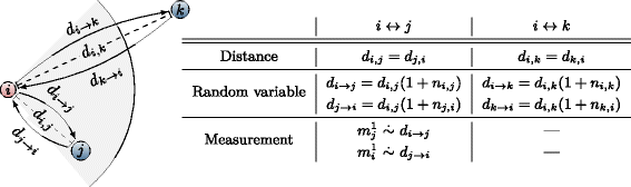
Illustration of the notation and the effects of the transmit ambiguities. Considered here are an agent i, which is assumed to use ID \(I_{\mathcal {R}}\) (red), and two surrounding agents (using ID \(I_{\mathcal {B}}\) (blue)), of which one is within the communication range of i. Also illustrated are the actual distances between i and the other two agents and the RVs that describe potential measurements of those distances. For both cases, the table given on the right-hand side clarifies the notation and the fact that no measurement of the distance between i and k has been made. Here, \(m\dot {\sim } d\) is used to denote that measurement m is a single realization, i.e., a sample, of the distribution d
Note that each measurement belongs to exactly one set of type \(\mathcal {V}_{1,a}(\cdot {},\cdot {})\) and one of type \(\mathcal {V}_{1,b}(\cdot {},\cdot {})\), as each vertex corresponds to two distance measurements. Because the solution to the TARP is given in the form of vertices (pairs of measurements) and because every measurement must be mapped exactly once, the size of the independent set corresponds to the number of sets of type \(\mathcal {E}_{1,a}(\cdot {},\cdot {})\), which is equal to the number of sets of type \(\mathcal {E}_{1,b}(\cdot {},\cdot {})\).
Note that items 1(a), 1(b), and 2, as listed in Section 3, introduce edges among specified sets of vertices. These vertices form the cliques.
In the following, the term tree node is used to refer to a vertex of the tree, whereas a subgraph is the graph that is induced by the edge and vertex sets at a given tree node.
Fig. 4 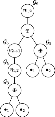
CW2-expressions and their corresponding 2-labeled graphs [20]
An induced subgraph consists of a subset of the vertex set of the graph and all edges whose endpoints are both in the vertex set [27].
For simplicity, and with a slight misuse of common terminology, we also refer to single vertices as cliques.
This becomes apparent when one notices that the CW k -tree needs to reflect an increasing number of the properties of the original graph as the considered tree node becomes closer to the root of the tree. At the root of the tree, the original graph must be obtained. Ensuring that the subgraphs are induced at each tree node is an easy way to satisfy this requirement.
Note that this algorithm is easily parallelizable by virtue of the tree structure.
Assume, e.g., dnext = anext + bmin, and let
 and
and  denote the label sets corresponding to anext and bmin, respectively. If
  and
and  are feasible with respect to Problem (18) at tree node s, then the bound dnext is tight.


 and
and  denote the label sets corresponding to anext and bmin, respectively. If
  and
and  are feasible with respect to Problem (18) at tree node s, then the bound dnext is tight.
Abbreviations
- BT:
-
Backtracking
- CHOPS:
-
Cold heavy oil production with sand
- CW:
-
Clique-width
- DS-CDMA:
-
Direct-Sequence (Spread Spectrum) Code-Division Multiple Access
- FDMA:
-
Frequency-division multiple access
- FPT:
-
Fixed-parameter tractability
- ID:
-
Identification number or sequence
- ILP:
-
Integer linear program
- MW-ISP-SC:
-
Minimum-weight independent set problem with size constraints
- MMSE:
-
Minimum mean-squared error
- MAP:
-
Maximum a posteriori
- RTT:
-
Round-trip time
- RV:
-
Random variable
- SN:
-
Serial number
- TA:
-
Transmit ambiguity
- TDMA:
-
Time-division multiple access
References
E Talnishnikh, J van Pol, HJ Wörtche, in Intelligent Environmental Sensing. Smart Sensors, Measurement and Instrumentation, 13, ed. by H Leung, S Chandra Mukhopadhyay. Micro motes: a highly penetrating probe for inaccessible environments (Springer International PublishingCham, 2015), pp. 33–49.
MB Dusseault, CHOPS—cold heavy oil production with sand in the Canadian heavy oil industry (2004). https://open.alberta.ca/dataset/2815953.
P Biswas, Y Ye, in Information Processing in Sensor Networks, 2004. IPSN 2004. Third International Symposium On. Semidefinite programming for ad hoc wireless sensor network localization, (2004), pp. 46–54. https://doi.org/10.1109/IPSN.2004.1307322.
AM-C So, Y Ye, in Proceedings of the Sixteenth Annual ACM-SIAM Symposium on Discrete Algorithms (SODA), 2005. Theory of semidefinite programming for sensor network localization (Society for Industrial and Applied MathematicsPhiladelphia, 2005), pp. 405–414.
Z Wang, S Zheng, S Boyd, Y Ye, Further relaxations of the sdp approach to sensor network localization (2006). Technical report.
P Biswas, T-C Lian, T-C Wang, Y Ye, Semidefinite programming based algorithms for sensor network localization. ACM Trans. Sen. Netw.2(2), 188–220 (2006). https://doi.org/10.1145/1149283.1149286.
P Biswas, T-C Liang, K-C Toh, Y Ye, T-C Wang, Semidefinite programming approaches for sensor network localization with noisy distance measurements. 3(4), 360–371 (2006). https://doi.org/10.1109/TASE.2006.877401.
H Chen, G Wang, Z Wang, HC So, HV Poor, Non-line-of-sight node localization based on semi-definite programming in wireless sensor networks. IEEE Trans. Wireless Commun.11(1), 108–116 (2012). https://doi.org/10.1109/TWC.2011.110811.101739.
Q Shi, C He, H Chen, L Jiang, Distributed wireless sensor network localization via sequential greedy optimization algorithm. IEEE Trans. Signal Process.58(6), 3328–3340 (2010). https://doi.org/10.1109/TSP.2010.2045416.
P Tseng, Second-order cone programming relaxation of sensor network localization. SIAM J. Optim.18(1), 156–185 (2007). https://doi.org/10.1137/050640308.
GC Calafiore, L Carlone, M Wei, in 18th Mediterranean Conference on Control Automation (MED), 2010. Position estimation from relative distance measurements in multi-agents formations, (2010), pp. 148–153. https://doi.org/10.1109/MED.2010.5547601.
B Liu, H Chen, Z Zhong, HV Poor, Asymmetrical round trip based synchronization-free localization in large-scale underwater sensor networks. IEEE Trans. Wireless Commun.9(11), 3532–3542 (2010). https://doi.org/10.1109/TWC.2010.090210.100146.
E Duisterwinkel, L Demi, G Dubbelman, E Talnishnikh, HJ Wörtche, JW Bergmans, Environment mapping and localization with an uncontrolled swarm of ultrasound sensor motes. Proc. Meet. Acoust.20(1), 030001 (2013). https://doi.org/10.1121/1.4879264.
S Schlupkothen, G Ascheid, in 2015 14th Annual Mediterranean Ad Hoc Networking Workshop (MED-HOC-NET) (Med-Hoc-Net’15). Localization of wireless sensor networks with concurrently used identification sequences (Vilamoura, Portugal, 2015), pp. 1–7. https://doi.org/10.1109/MedHocNet.2015.7173166.
S Schlupkothen, G Ascheid, in 2016 IEEE International Conference on Wireless for Space and Extreme Environments (WiSEE). Joint localization and transmit-ambiguity resolution for ultra-low energy wireless sensors, (2016), pp. 48–53. https://doi.org/10.1109/WiSEE.2016.7877302.
S Schlupkothen, B Prasse, G Ascheid, in 2016 Mediterranean Ad Hoc Networking Workshop (Med-Hoc-Net). A dynamic programming algorithm for resolving transmit-ambiguities in the localization of wsn, (2016), pp. 1–8. https://doi.org/10.1109/MedHocNet.2016.7528420.
CA Floudas, PM Pardalos, Encyclopedia of Optimization, Second Edition (Springer, Secaucus, 2009).
DZ Du, KI Ko, Theory of Computational Complexity. Wiley Series in Discrete Mathematics and Optimization (Wiley, New York, 2011).
J Flum, M Grohe, Parameterized Complexity Theory. Texts in Theoretical Computer Science. An EATCS Series (Springer, Berlin Heidelberg, 2006).
F Gurski, I Rothe, J Rothe, E Wanke, Exakte Algorithmen Für Schwere Graphenprobleme. eXamen.press (Springer, Berlin Heidelberg, 2010).
F Gurski, A comparison of two approaches for polynomial time algorithms computing basic graph parameters. CoRR. abs/0806.4073: (2008). http://arxiv.org/abs/0806.4073.
S Oum, SH Sæther, M Vatshelle, Faster algorithms for vertex partitioning problems parameterized by clique-width. Theor. Comput. Sci.535:, 16–24 (2014).
MR Fellows, FA Rosamond, U Rotics, S Szeider, Clique-width is np-complete. SIAM J. Discrete Math.23(2), 909–939 (2009). https://doi.org/10.1137/070687256.
HL Bodlaender, A tourist guide through treewidth. Acta Cybern. 11(1-2), 1–21 (1993).
B Courcelle, S Olariu, Upper bounds to the clique width of graphs. Discrete Appl. Math.101(1–3), 77–114 (2000).
W Espelage, F Gurski, E Wanke, in Algorithms and Data Structures: 7th International Workshop, WADS 2001 Providence, RI, USA, August 8–10, 2001 Proceedings, ed. by F Dehne, J-R Sack, and R Tamassia. Deciding clique-width for graphs of bounded tree-width (SpringerBerlin, Heidelberg, 2001), pp. 87–98.
EW Weisstein, Vertex-induced subgraph. From MathWorld—A Wolfram Web Resource (2016). Last visited on 02/02/2016. http://mathworld.wolfram.com/Vertex-InducedSubgraph.html.
M Tawarmalani, NV Sahinidis, A polyhedral branch-and-cut approach to global optimization. Math. Program.103:, 225–249 (2005).
N Patwari, AO Hero III, in Proceedings of the 2Nd ACM International Conference on Wireless Sensor Networks and Applications. WSNA ’03. Using proximity and quantized rss for sensor localization in wireless networks (ACMNew York, 2003), pp. 20–29. https://doi.org/10.1145/941350.941354.
JA Costa, N Patwari, AO Hero III, Distributed weighted-multidimensional scaling for node localization in sensor networks. ACM Trans. Sen. Netw.2(1), 39–64 (2006). https://doi.org/10.1145/1138127.1138129.
EW Weisstein, Normal difference distribution. From MathWorld—A Wolfram Web Resource (2016). http://mathworld.wolfram.com/NormalDifferenceDistribution.html. Accessed 02 Feb 2016.
A Goldsmith, Wireless Communications (Cambridge University Press, New York, 2005).
Acknowledgements
We gratefully acknowledge the computational resources provided by the RWTH Compute Cluster from RWTH Aachen University under project RWTH0118.
Funding
This project has received funding from the European Union’s Horizon 2020 research and innovation program under grant agreement no. 665347.
Author information
Authors and Affiliations
Contributions
All authors contributed equally to this work. All authors read and approved the final manuscript.
Corresponding author
Ethics declarations
Competing interests
The authors declare that they have no competing interests.
Publisher’s Note
Springer Nature remains neutral with regard to jurisdictional claims in published maps and institutional affiliations.
Rights and permissions
Open Access This article is distributed under the terms of the Creative Commons Attribution 4.0 International License (http://creativecommons.org/licenses/by/4.0/), which permits unrestricted use, distribution, and reproduction in any medium, provided you give appropriate credit to the original author(s) and the source, provide a link to the Creative Commons license, and indicate if changes were made.
About this article

Cite this article
Schlupkothen, S., Prasse, B. & Ascheid, G. Backtracking-based dynamic programming for resolving transmit ambiguities in WSN localization. EURASIP J. Adv. Signal Process. 2018, 20 (2018). https://doi.org/10.1186/s13634-018-0536-x
Received:
Accepted:
Published:
DOI: https://doi.org/10.1186/s13634-018-0536-x