A new more accurate half-discrete Hilbert-type inequality

Abstract

By using the way of weight functions and the idea of introducing parameters and by means of Hadamard’s inequality, we give a more accurate half-discrete Hilbert-type inequality with a best constant factor. We also consider its best extension with parameters, equivalent forms, operator expressions as well as some reverses.

MSC:26D15, 47A07.

1 Introduction

If $p>1$, $\frac{1}{p}+\frac{1}{q}=1$, $a_n,b_n\ge 0$, such that $0<{\sum }_{n=1}^{\mathrm{\infty }}{a}_n^p<\mathrm{\infty }$ and $0<{\sum }_{n=1}^{\mathrm{\infty }}{b}_n^q<{\mathrm{\infty }}_{,}$ then we have the following famous Hilbert-type integral inequality (cf. [1]):

$$\sum _{n=1}^{\mathrm{\infty }}\sum _{m=1}^{\mathrm{\infty }}\frac{ln(m/n)}{m-n}{a}_m{b}_n<{\left[\frac{\pi }{sin(\pi /p)}\right]}^2{\left\{\sum _{n=1}^{\mathrm{\infty }}{a}_n^p\right\}}^{\frac{1}{p}}{\left\{\sum _{n=1}^{\mathrm{\infty }}{b}_n^q\right\}}^{\frac{1}{q}},$$

(1)

where the constant factor ${[\pi /sin(\pi /p)]}^2$ is the best possible. The integral analogue of inequality (1) is given as follows (cf. [1]). If $p>1$, $\frac{1}{p}+\frac{1}{q}=1$, $f(x)$ and $g(x)$ are non-negative real functions such that $0<{\int }_0^{\mathrm{\infty }}{f}^p(x)dx<\mathrm{\infty }$ and $0<{\int }_0^{\mathrm{\infty }}{g}^q(x)dx<\mathrm{\infty }$, then

(2)

where the constant factor ${[\pi /sin(\pi /p)]}^2$ is the best possible. We named inequality (2) Hilbert-type integral inequality. In 2007, Yang proved the following more accurate Hilbert-type inequality (cf. [2]). If $p>1$, $\frac{1}{p}+\frac{1}{q}=1$, $\frac{1}{2}\le \alpha \le 1$, $a_n,b_n\ge 0$, such that $0<{\sum }_{n=0}^{\mathrm{\infty }}{a}_n^p<\mathrm{\infty }$ and $0<{\sum }_{n=0}^{\mathrm{\infty }}{b}_n^q<\mathrm{\infty }$, then

$$\sum _{n=0}^{\mathrm{\infty }}\sum _{m=0}^{\mathrm{\infty }}\frac{ln(\frac{m+\alpha }{n+\alpha })}{m-n}{a}_m{b}_n<{\left[\frac{\pi }{sin(\pi /p)}\right]}^2{\left\{\sum _{n=0}^{\mathrm{\infty }}{a}_n^p\right\}}^{\frac{1}{p}}{\left\{\sum _{n=0}^{\mathrm{\infty }}{b}_n^q\right\}}^{\frac{1}{q}},$$

(3)

where the constant factor ${[\pi /sin(\pi /p)]}^2$ is still the best possible. Inequalities (1)-(3) are important in mathematical analysis and its applications [3]. There are lots of improvements, generalizations, and applications of inequalities (1)-(3); for more details, refer to [4–17].

At present, the research into half-discrete Hilbert-type inequalities is a new direction and has gradually heated up. We find a few results on the half-discrete Hilbert-type inequalities with the non-homogeneous kernel, which were published earlier (cf. [1], Th. 351 and [18]). Recently, Yang has given some half-discrete Hilbert-type inequalities (cf. [19–25]). Zhong proved a half-discrete Hilbert-type inequality with the non-homogeneous kernel as follows (cf. [26]). If $p>1$, $\frac{1}{p}+\frac{1}{q}=1$, $0<\lambda \le 2$, $a_n,f(x)\ge 0$, $f(x)$ is a measurable function in $(0,\mathrm{\infty })$ such that $0<{\sum }_{n=1}^{\mathrm{\infty }}{n}^{p(1-\frac{\lambda }{2})-1}{a}_n^p<\mathrm{\infty }$ and $0<{\int }_0^{\mathrm{\infty }}{x}^{q(1-\frac{\lambda }{2})-1}{f}^q(x)dx<\mathrm{\infty }$, then

(4)

where the constant factor ${(\frac{\pi }{\lambda })}^2$ is the best possible.

In this paper, by using the way of weight functions and the idea of introducing parameters and by means of Hadamard’s inequality, we give a half-discrete Hilbert-type inequality with a best constant factor as follows:

$$\sum _{n=1}^{\mathrm{\infty }}{a}_n{\int }_0^{\mathrm{\infty }}\frac{ln(\frac{x}{n})}{x-n}f(x)dx<{\pi }^2{(\sum _{n=1}^{\mathrm{\infty }}{a}_n^2{\int }_0^{\mathrm{\infty }}{f}^2(x)dx)}^{\frac{1}{2}}.$$

(5)

The main objective of this paper is to consider its more accurate extension with parameters, equivalent forms, operator expressions as well as some reverses.

2 Some lemmas

Lemma 1 If $r>1$, $\frac{1}{r}+\frac{1}{s}=1$, define the following beta function (cf. [1]):

$${\int }_0^{\mathrm{\infty }}\frac{lnu}{u-1}{u}^{\frac{1}{s}-1}du={\left[B(\frac{1}{s},\frac{1}{r})\right]}^2={\left(\frac{\pi }{sin\frac{\pi }{s}}\right)}^2.$$

(6)

Lemma 2 Suppose that $r>1$, $\frac{1}{r}+\frac{1}{s}=1$, $0\le \beta \le \frac{1}{2}$, $\nu \in (-\mathrm{\infty },\mathrm{\infty })$, $0<\lambda \le 1$. Define the weight functions $\omega (n)$ and $\tilde{\omega }(x)$ as follows:

(7)

(8)

Setting $k_{\lambda }(r):={[\frac{\pi }{\lambda sin(\frac{\pi }{r})}]}^2$, we have the following inequalities:

(9)

(10)

Proof Putting $u={(\frac{x-\nu }{n-\beta })}^{\lambda }$ in (8), we have

$$\begin{array}{rcl}{\omega }_{\lambda }(n)& =& \frac{1}{{\lambda }^2}{\int }_0^{\mathrm{\infty }}\frac{lnu}{u-1}{u}^{\frac{1}{s}-1}du=\frac{1}{{\lambda }^2}{\left[B(\frac{1}{s},\frac{1}{r})\right]}^2\\ =& \frac{1}{{\lambda }^2}{\left[B(\frac{1}{r},\frac{1}{s})\right]}^2={\left[\frac{\pi }{\lambda sin(\frac{\pi }{r})}\right]}^2=k_{\lambda }(r).\end{array}$$

(11)

For fixed $x\in (\nu ,\mathrm{\infty })$, setting

$$f(t):=\frac{{(x-\nu )}^{\frac{\lambda }{s}}ln(\frac{x-\nu }{t-\beta })}{{(x-\nu )}^{\lambda }-{(t-\beta )}^{\lambda }}{(t-\beta )}^{\frac{\lambda }{r}-1}(t\in (\beta ,\mathrm{\infty })),$$

(12)

in view of the conditions, we find $f^{\mathrm{\prime }}(t)<0$ and $f^{\mathrm{\prime }\mathrm{\prime }}(t)>0$ (cf. [27]). By Hadamard’s inequality (cf. [28]),

$$f(n)<{\int }_{n-\frac{1}{2}}^{n+\frac{1}{2}}f(t)dt(n\in \mathbf{N}),$$

(13)

and putting $v={(\frac{t-\beta }{x-\nu })}^{\lambda }$, we obtain

$$\begin{array}{rcl}{\tilde{\omega }}_{\lambda }(x)& =& \sum _{n=1}^{\mathrm{\infty }}f(n)<\sum _{n=1}^{\mathrm{\infty }}{\int }_{n-\frac{1}{2}}^{n+\frac{1}{2}}f(t)dt={\int }_{\frac{1}{2}}^{\mathrm{\infty }}f(t)dt\\ \le & {\int }_{\beta }^{\mathrm{\infty }}f(t)dt=\frac{1}{{\lambda }^2}{\int }_0^{\mathrm{\infty }}\frac{lnv}{v-1}{v}^{\frac{1}{r}-1}du=k_{\lambda }(r),\\ {\tilde{\omega }}_{\lambda }(x)& =& \sum _{n=1}^{\mathrm{\infty }}f(n)>{\int }_1^{\mathrm{\infty }}f(t)dt={\int }_{\beta }^{\mathrm{\infty }}f(t)dt-{\int }_{\beta }^{1}f(t)dt\\ =& k_{\lambda }(r)-\frac{1}{{\lambda }^2}{\int }_0^{{(\frac{1-\beta }{x-\nu })}^{\lambda }}\frac{lnv}{v-1}{v}^{\frac{1}{r}-1}dv=k_{\lambda }(r)(1-{\theta }_{\lambda }(x))>0,\end{array}$$

where,

$$0<{\theta }_{\lambda }(x):={\left[\frac{sin(\frac{\pi }{r})}{\pi }\right]}^2{\int }_0^{{(\frac{1-\beta }{x-\nu })}^{\lambda }}\frac{lnv}{v-1}{v}^{\frac{1}{r}-1}dv(x\in (\nu ,\mathrm{\infty })).$$

Since ${lim}_{v\to 0^{+}}\frac{lnv}{v-1}{v}^{\frac{1}{2r}}={lim}_{v\to \mathrm{\infty }}\frac{lnv}{v-1}{v}^{\frac{1}{2r}}=0$ and $\frac{lnv}{v-1}{v}^{\frac{1}{2r}}{\mid }_{v=1}=1$, in view of the bounded properties of a continuous function, there exists $M>0$ such that $0<\frac{lnv}{v-1}{v}^{\frac{1}{2r}}\le M$ ($v\in (0,\mathrm{\infty })$). For $x\in (\nu ,\mathrm{\infty })$, we have

$$\begin{array}{rcl}0& <& {\int }_0^{{(\frac{1-\beta }{x-\nu })}^{\lambda }}\frac{lnv}{v-1}{v}^{\frac{1}{r}-1}dv={\int }_0^{{(\frac{1-\beta }{x-\nu })}^{\lambda }}\frac{lnv}{v-1}{v}^{\frac{1}{2r}}\cdot v^{\frac{1}{2r}-1}dv\\ \le & M{\int }_0^{{(\frac{1-\beta }{x-\nu })}^{\lambda }}{v}^{\frac{1}{2r}-1}dv=\frac{2Mr{(1-\beta )}^{\lambda /2r}}{{(x-\nu )}^{\lambda /2r}}.\end{array}$$

(14)

Hence, we proved that (9) and (10) are valid. □

Lemma 3 Suppose that $r>1$, $\frac{1}{r}+\frac{1}{s}=1$, $\frac{1}{p}+\frac{1}{q}=1$ ($p\ne 0,1$), $0\le \beta \le \frac{1}{2}$, $\nu \in (-\mathrm{\infty },\mathrm{\infty })$, $0<\lambda \le 1$, $a_n\ge 0$, and $f(x)$ is a non-negative real measurable function in $(\nu ,\mathrm{\infty })$. Then

• (i) for $p>1$, we have the following inequalities:

  

  (15)

(16)

where ${\omega }_{\lambda }(n)$ and ${\tilde{\omega }}_{\lambda }(x)$ are defined by (7) and (8).

• (ii) for $p<1$ ($p\ne 0$), we have the reverses of (15) and (16).

Proof (i) By (7)-(10) and Hölder’s inequality [28], we have

(17)

By the Lebesgue term-by-term integration theorem [29] and (9), we obtain

$$\begin{array}{rcl}{J}^p& \le & k_{\lambda }^{p-1}(r)\sum _{n=1}^{\mathrm{\infty }}{\int }_{\nu }^{\mathrm{\infty }}\frac{f^p(x)ln(\frac{x-\nu }{n-\beta })}{{(x-\nu )}^{\lambda }-{(n-\beta )}^{\lambda }}\frac{{(x-\nu )}^{(1-\frac{\lambda }{s})(p-1)}}{{(n-\beta )}^{1-\frac{\lambda }{r}}}dx\\ =& k_{\lambda }^{p-1}(r){\int }_{\nu }^{\mathrm{\infty }}\sum _{n=1}^{\mathrm{\infty }}\frac{{(n-\beta )}^{\frac{\lambda }{r}-1}ln(\frac{x-\nu }{n-\beta })}{{(x-\nu )}^{\lambda }-{(n-\beta )}^{\lambda }}{(x-\nu )}^{\frac{\lambda }{s}+p(1-\frac{\lambda }{s})-1}{f}^p(x)dx\\ =& k_{\lambda }^{p-1}(r){\int }_{\nu }^{\mathrm{\infty }}{\tilde{\omega }}_{\lambda }(x){(x-\nu )}^{p(1-\frac{\lambda }{s})-1}{f}^p(x)dx.\end{array}$$

(18)

Hence, (15) is valid. Using Hölder’s inequality, the Lebesgue term-by-term integration theorem, and (9) again, we have

(19)

(20)

Hence, (16) is valid.

• (ii) For $0<p<1$ ($q<0$) or $p<0$ ($0<q<1$), using the reverse Hölder inequality, in the same way, we obtain the reverses of (15) and (16). □

Lemma 4 By the assumptions of Lemma  2 and Lemma  3, we set $\varphi (x):={(x-\nu )}^{p(1-\frac{\lambda }{s})-1}$, $\tilde{\varphi }(x):=(1-{\theta }_{\lambda }(x))\varphi (x)$, $\psi (n):={(n-\beta )}^{q(1-\frac{\lambda }{r})-1}$,

(Note If $p>1$, then $L_{p,\varphi }(\nu ,\mathrm{\infty })$ and $l_{q,\psi }$ are normal spaces; if $0<p<1$ or $p<0$, then both $L_{p,\varphi }(\nu ,\mathrm{\infty })$ and $l_{q,\psi }$ are not normal spaces, but we still use the formal symbols in the following.)

For $0<\epsilon <\frac{|p|\lambda }{s}$, setting $\tilde{a}={\{{\tilde{a}}_n\}}_{n=1}^{\mathrm{\infty }}$, and $\tilde{f}(x)$ as follows:

$${\tilde{a}}_n={(n-\beta )}^{\frac{\lambda }{r}-\frac{\epsilon }{q}-1};\tilde{f}(x)=\{\begin{array}{cc}0,\hfill & x\in (\nu ,1+\nu ),\hfill \\ {(x-\nu )}^{\frac{\lambda }{s}-\frac{\epsilon }{p}-1},\hfill & x\in [1+\nu ,\mathrm{\infty }),\hfill \end{array}$$

(21)

• (i) if $p>1$, there exists a constant $k>0$ such that

  $$\tilde{I}:=\sum _{n=1}^{\mathrm{\infty }}{\tilde{a}}_n{\int }_{\nu }^{\mathrm{\infty }}\frac{ln(\frac{x-\nu }{n-\beta })}{{(x-\nu )}^{\lambda }-{(n-\beta )}^{\lambda }}\tilde{f}(x)dx<k{\parallel \tilde{f}\parallel }_{p,\varphi }{\parallel \tilde{a}\parallel }_{q,\psi },$$

  (22)

then it follows

$$\begin{array}{rcl}k{\left[\frac{\epsilon +1-\beta }{{(1-\beta )}^{\epsilon +1}}\right]}^{1/q}& >& \frac{1}{{\lambda }^2{(1-\beta )}^{\epsilon }}{\int }_0^{{(1-\beta )}^{\lambda }}\frac{lnt}{t-1}{t}^{\frac{1}{r}+\frac{\epsilon }{p\lambda }-1}dt\\ +\frac{1}{{\lambda }^2}{\int }_{{(1-\beta )}^{\lambda }}^{\mathrm{\infty }}\frac{lnt}{t-1}{t}^{\frac{1}{r}-\frac{\epsilon }{q\lambda }-1}dt;\end{array}$$

(23)

• (ii) if $0<p<1$, there exists a constant $k>0$ such that

  $$\tilde{I}=\sum _{n=1}^{\mathrm{\infty }}{\tilde{a}}_n{\int }_{\nu }^{\mathrm{\infty }}\frac{ln(\frac{x-\nu }{n-\beta })}{{(x-\nu )}^{\lambda }-{(n-\beta )}^{\lambda }}\tilde{f}(x)dx>k{\parallel \tilde{f}\parallel }_{p,\tilde{\varphi }}{\parallel \tilde{a}\parallel }_{q,\psi },$$

  (24)

then it follows

$$k{(1-\epsilon O(1))}^{1/p}<\frac{1}{{\lambda }^2}{\left[\frac{\epsilon +1-\beta }{{(1-\beta )}^{\epsilon +1}}\right]}^{1/p}{\left[B(\frac{1}{s}-\frac{\epsilon }{p\lambda },\frac{1}{r}+\frac{\epsilon }{p\lambda })\right]}^2;$$

(25)

• (iii) if $p<0$, there exists a constant $k>0$ such that

  $$\tilde{I}=\sum _{n=1}^{\mathrm{\infty }}{\tilde{a}}_n{\int }_{\nu }^{\mathrm{\infty }}\frac{ln(\frac{x-\nu }{n-\beta })}{{(x-\nu )}^{\lambda }-{(n-\beta )}^{\lambda }}\tilde{f}(x)dx>k{\parallel \tilde{f}\parallel }_{p,\varphi }{\parallel \tilde{a}\parallel }_{q,\psi },$$

  (26)

then it follows

$$k{\left[\frac{1}{{(1-\beta )}^{\epsilon }}\right]}^{1/q}<\frac{\epsilon +1-\beta }{{\lambda }^2{(1-\beta )}^{\epsilon +1}}{\left[B(\frac{1}{s}-\frac{\epsilon }{p\lambda },\frac{1}{r}+\frac{\epsilon }{p\lambda })\right]}^2.$$

(27)

Proof We can obtain

(28)

(29)

(30)

• (i) For $p>1$, then $q>1$, $\frac{\lambda }{r}-\frac{\epsilon }{q}-1<0$, by (22), (28), and (29), we find

  

  (31)

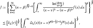
Setting $t={(\frac{y-\beta }{x-\nu })}^{\lambda }$, $z=x-v$ in the above integral, we have

$$\tilde{I}\ge \frac{1}{{\lambda }^2}{\int }_1^{\mathrm{\infty }}{z}^{-1-\epsilon }\left[{\int }_{{(\frac{1-\beta }{z})}^{\lambda }}^{\mathrm{\infty }}\frac{lnt}{t-1}{t}^{\frac{1}{r}-\frac{\epsilon }{q\lambda }-1}dt\right]dz=I_1+I_2,$$

(32)

and by the Fubini theorem [30], it follows

(33)

(34)

In view of (33) and (34), it follows that

$$\begin{array}{rcl}\tilde{I}& \ge & \frac{1}{\epsilon {\lambda }^2{(1-\beta )}^{\epsilon }}{\int }_0^{{(1-\beta )}^{\lambda }}\frac{lnt}{t-1}{t}^{\frac{1}{r}+\frac{\epsilon }{p\lambda }-1}dt\\ +\frac{1}{\epsilon {\lambda }^2}{\int }_{{(1-\beta )}^{\lambda }}^{\mathrm{\infty }}\frac{lnt}{t-1}{t}^{\frac{1}{r}-\frac{\epsilon }{q\lambda }-1}dt.\end{array}$$

(35)

Then by (31) and (35), (23) is valid.

• (ii) For $0<p<1$, by (24) and (29), we find (notice that $q<0$)

  $$\begin{array}{rcl}\tilde{I}& >& k{\parallel \tilde{f}\parallel }_{p,\tilde{\varphi }}{\parallel {\tilde{a}}_n\parallel }_{q,\psi }=k{\{{\int }_{\nu }^{\mathrm{\infty }}\tilde{\varphi }(x){|\tilde{f}(x)|}^{p}dx\}}^{1/p}{\parallel \tilde{a}\parallel }_{q,\psi }\\ =& k{\left\{{\int }_{1+\nu }^{\mathrm{\infty }}[1-O\left(\frac{1}{{(x-\nu )}^{\lambda /2r}}\right)]{(x-\nu )}^{-1-\epsilon }dx\right\}}^{1/p}{\parallel \tilde{a}\parallel }_{q,\psi }\\ =& k{[\frac{1}{\epsilon }-{\int }_{1+\nu }^{\mathrm{\infty }}O\left(\frac{1}{{(x-\nu )}^{\frac{\lambda }{2r}+\epsilon +1}}\right)dx]}^{1/p}{\parallel \tilde{a}\parallel }_{q,\psi }\\ >& k{[\frac{1}{\epsilon }-O(1)]}^{1/p}{\left[\frac{\epsilon +1-\beta }{\epsilon {(1-\beta )}^{\epsilon +1}}\right]}^{1/q}\\ =& \frac{k}{\epsilon }{[1-\epsilon O(1)]}^{1/p}{\left[\frac{\epsilon +1-\beta }{{(1-\beta )}^{\epsilon +1}}\right]}^{1/q}.\end{array}$$

  (36)

On the other hand, setting $t={(\frac{x-\nu }{n-\beta })}^{\lambda }$ in $\tilde{I}$, we have

$$\begin{array}{rcl}\tilde{I}& =& \sum _{n=1}^{\mathrm{\infty }}{(n-\beta )}^{\frac{\lambda }{r}-\frac{\epsilon }{q}-1}{\int }_{1+\nu }^{\mathrm{\infty }}\frac{ln(\frac{x-\nu }{n-\beta })}{{(x-\nu )}^{\lambda }-{(n-\beta )}^{\lambda }}{(x-\nu )}^{\frac{\lambda }{s}-\frac{\epsilon }{p}-1}dx\\ =& \frac{1}{{\lambda }^2}\sum _{n=1}^{\mathrm{\infty }}{(n-\beta )}^{-1-\epsilon }{\int }_{\frac{1}{{(n-\beta )}^{\lambda }}}^{\mathrm{\infty }}\frac{lnt}{t-1}{t}^{\frac{1}{s}-\frac{\epsilon }{p\lambda }-1}dt\\ <& \frac{1}{{\lambda }^2}\sum _{n=1}^{\mathrm{\infty }}{(n-\beta )}^{-1-\epsilon }{\int }_0^{\mathrm{\infty }}\frac{lnt}{t-1}{t}^{\frac{1}{s}-\frac{\epsilon }{p\lambda }-1}dt\\ <& \frac{\epsilon +1-\beta }{{\lambda }^2\epsilon {(1-\beta )}^{\epsilon +1}}{\left[B(\frac{1}{s}-\frac{\epsilon }{p\lambda },\frac{1}{r}+\frac{\epsilon }{p\lambda })\right]}^2.\end{array}$$

(37)

By virtue of (36) and (37), (25) is valid.

• (iii) For $p<0$, then $0<q<1$, by (26) and (30), we find

  $$\begin{array}{rcl}\tilde{I}& >& k{\{{\int }_{\nu }^{\mathrm{\infty }}\varphi (x){\tilde{f}}^p(x)dx\}}^{1/p}{\parallel \tilde{a}\parallel }_{q,\psi }=k{\left\{{\int }_{1+\nu }^{\mathrm{\infty }}{(x-\nu )}^{-1-\epsilon }dx\right\}}^{1/p}{\parallel \tilde{a}\parallel }_{q,\psi }\\ >& \frac{k}{\epsilon }{\left[\frac{1}{{(1-\beta )}^{\epsilon }}\right]}^{1/q}.\end{array}$$

  (38)

Then by (37) and (38), (27) is valid. □

3 Main results and applications

Theorem 5 Suppose that $p>1$, $\frac{1}{p}+\frac{1}{q}=1$, $r>1$, $\frac{1}{r}+\frac{1}{s}=1$, $0<\lambda \le 1$, $0\le \beta \le \frac{1}{2}$, $\nu \in (-\mathrm{\infty },+\mathrm{\infty })$, $\varphi (x):={(x-\nu )}^{p(1-\frac{\lambda }{s})-1}$, $\psi (n):={(n-\beta )}^{q(1-\frac{\lambda }{r})-1}$, $f(x),a_n\ge 0$, satisfying $f\in L_{p,\varphi }(\nu ,\mathrm{\infty })$, $a={\{a_n\}}_{n=1}^{\mathrm{\infty }}\in l_{q,\psi }$, ${\parallel f\parallel }_{p,\varphi }>0$, ${\parallel a\parallel }_{q,\psi }>0$, then we have the following equivalent inequalities:

(39)

(40)

(41)

where the constant factor $k_{\lambda }(r)={[\frac{\pi }{\lambda sin(\frac{\pi }{r})}]}^2$ is the best possible.

Proof By the Lebesgue term-by-term integration theorem [29], we find that there are two expressions of I in (39). By (9), (15), and $0<{\parallel f\parallel }_{p,\varphi }<\mathrm{\infty }$, we have (40). By Hölder’s inequality, we find

$$\begin{array}{rcl}I& =& \sum _{n=1}^{\mathrm{\infty }}\left[{(n-\beta )}^{\frac{\lambda }{r}-\frac{1}{p}}{\int }_{\nu }^{\mathrm{\infty }}\frac{ln(\frac{x-\nu }{n-\beta })f(x)}{{(x-\nu )}^{\lambda }-{(n-\beta )}^{\lambda }}dx\right]\left[{(n-\beta )}^{\frac{1}{p}-\frac{\lambda }{r}}{a}_n\right]\\ \le & J{\{\sum _{n=1}^{\mathrm{\infty }}[{(n-\beta )}^{q(1-\frac{\lambda }{r})-1}{a}_n^q\}}^{1/q}=J{\parallel a\parallel }_{q,\psi }.\end{array}$$

(42)

Then by (40), (39) is valid. On the other hand, assuming that (39) is valid, set

$$a_n:={(n-\beta )}^{\frac{p\lambda }{r}-1}{[{\int }_{\nu }^{\mathrm{\infty }}\frac{ln(\frac{x-\nu }{n-\beta })}{{(x-\nu )}^{\lambda }-{(n-\beta )}^{\lambda }}f(x)dx]}^{p-1}(n\in \mathbf{N}).$$

(43)

Then by (39), we have

$${\parallel a\parallel }_{q,\psi }^q=\sum _{n=1}^{\mathrm{\infty }}{(n-\beta )}^{q(1-\frac{\lambda }{r})-1}{a}_n^q=J^p=I\le k_{\lambda }(r){\parallel f\parallel }_{p,\varphi }{\parallel a\parallel }_{q,\psi }.$$

(44)

By (9), (15), and $0<{\parallel f\parallel }_{p,\varphi }<\mathrm{\infty }$, it follows that $J<\mathrm{\infty }$. If $J=0$, then (40) is trivially valid; if $J>0$, then $0<{\parallel a\parallel }_{q,\psi }=J^{p-1}<\mathrm{\infty }$. Thus, the conditions of applying (39) are fulfilled, and by (39), (44) takes a strict sign inequality. Thus, we find

$$J={\parallel a\parallel }_{q,\psi }^{q-1}<k_{\lambda }(r){\parallel f\parallel }_{p,\varphi }.$$

(45)

Hence, (40) is valid, which is equivalent to (39).

By (9), (16), and $0<{\parallel a\parallel }_{q,\psi }<\mathrm{\infty }$, we obtain (41). By Hölder’s inequality again, we have

$$\begin{array}{rcl}I& =& {\int }_{\nu }^{\mathrm{\infty }}\left[{(x-\nu )}^{\frac{\lambda }{s}-\frac{1}{q}}\sum _{n=1}^{\mathrm{\infty }}\frac{ln(\frac{x-\nu }{n-\beta })}{{(x-\nu )}^{\lambda }-{(n-\beta )}^{\lambda }}{a}_n\right][{(x-\nu )}^{\frac{1}{q}-\frac{\lambda }{s}}f(x)]dx\\ \le & L{\{{\int }_{\nu }^{\mathrm{\infty }}{(x-\nu )}^{p(1-\frac{\lambda }{s})-1}{f}^p(x)dx\}}^{1/p}=L{\parallel f\parallel }_{p,\varphi }.\end{array}$$

(46)

Hence, (39) is valid by using (41). On the other hand, assuming that (39) is valid, set

$$f(x):={(x-\nu )}^{\frac{q\lambda }{s}-1}{\left[\sum _{n=1}^{\mathrm{\infty }}\frac{ln(\frac{x-\nu }{n-\beta })}{{(x-\nu )}^{\lambda }-{(n-\beta )}^{\lambda }}{a}_n\right]}^{q-1}(x\in (\nu ,\mathrm{\infty })).$$

(47)

Then by (39), we find

$${\parallel f\parallel }_{p,\varphi }^p={\int }_{\nu }^{\mathrm{\infty }}{(x-\nu )}^{p(1-\frac{\lambda }{s})-1}{f}^p(x)dx=L^q=I\le k_{\lambda }(r){\parallel f\parallel }_{p,\varphi }{\parallel a\parallel }_{q,\psi }.$$

(48)

By (9), (16), and $0<{\parallel a\parallel }_{q,\psi }<\mathrm{\infty }$, it follows that $L<\mathrm{\infty }$. If $L=0$, then (41) is trivially valid; if $L>0$, then $0<{\parallel f\parallel }_{p,\varphi }=L^{q-1}<\mathrm{\infty }$, i.e., the conditions of applying (39) are fulfilled and by (48), we still have

Hence, (41) is valid, which is equivalent to (39). It follows that (39), (40), and (41) are equivalent.

If there exits a positive number $k\le k_{\lambda }(r)$ such that (39) is still valid as we replace $k_{\lambda }(r)$ by k, then, in particular, (22) is valid (${\tilde{a}}_n,\tilde{f}(x)$ are taken as (21)). Then we have (23). By (11), the Fatou lemma [30], and (23), we have

$$\begin{array}{rcl}{k}_{\lambda }(r)& =& \frac{1}{{\lambda }^2}{\int }_0^{\mathrm{\infty }}\frac{lnt}{t-1}{t}^{\frac{1}{r}-1}dt\\ =& {\int }_0^{{(1-\beta )}^{\lambda }}\underset{\epsilon \to 0^{+}}{lim}\frac{lnt}{t-1}{t}^{\frac{1}{r}+\frac{\epsilon }{p\lambda }-1}dt+{\int }_{{(1-\beta )}^{\lambda }}^{\mathrm{\infty }}\underset{\epsilon \to 0^{+}}{lim}\frac{lnt}{t-1}{t}^{\frac{1}{r}-\frac{\epsilon }{q\lambda }-1}dt\\ \le & \underset{\epsilon \to 0^{+}}{\underline{lim}}[{\int }_0^{{(1-\beta )}^{\lambda }}\frac{lnt}{t-1}{t}^{\frac{1}{r}+\frac{\epsilon }{p\lambda }-1}dt+{\int }_{{(1-\beta )}^{\lambda }}^{\mathrm{\infty }}\frac{lnt}{t-1}{t}^{\frac{1}{r}-\frac{\epsilon }{q\lambda }-1}dt]\\ \le & \underset{\epsilon \to 0^{+}}{\underline{lim}}k{\left[\frac{\epsilon +1-\beta }{{(1-\beta )}^{\epsilon +1}}\right]}^{1/q}=k.\end{array}$$

Hence, $k=k_{\lambda }(r)$ is the best value of (39). We confirm that the constant factor $k_{\lambda }(r)$ in (40) ((41)) is the best possible. Otherwise, we can get a contradiction by (42) ((46)) that the constant factor in (39) is not the best possible. □

Remark 6 (i) Define a half-discrete Hilbert operator $T:L_{p,\varphi }(\nu ,\mathrm{\infty })\to l_{p,{\psi }^{1-p}}$ as follows. For $f\in L_{p,\varphi }(\nu ,\mathrm{\infty })$, we define $Tf\in l_{p,{\psi }^{1-p}}$ satisfying

$$Tf(n)={\int }_{\nu }^{\mathrm{\infty }}\frac{ln(\frac{x-\nu }{n-\beta })}{{(x-\nu )}^{\lambda }-{(n-\beta )}^{\lambda }}f(x)dx(n\in \mathbf{N}).$$

Then by (40), it follows ${\parallel Tf\parallel }_{p,{\psi }^{1-p}}\le k_{\lambda }(r){\parallel f\parallel }_{p,\varphi }$, i.e., T is the bounded operator with $\parallel T\parallel \le k_{\lambda }(r)$. Since the constant factor $k_{\lambda }(r)$ in (40) is the best possible, we have $\parallel T\parallel =k_{\lambda }(r)$.

• (ii) Define a half-discrete Hilbert operator $\tilde{T}:l_{q,\psi }\to L_{q,{\varphi }^{1-q}}(\nu ,\mathrm{\infty })$ in the following way. For $a\in l_{q,\psi }$, we define $\tilde{T}a\in L_{q,{\varphi }^{1-q}}(\nu ,\mathrm{\infty })$ satisfying

  $$\tilde{T}a(x)=\sum _{n=1}^{\mathrm{\infty }}\frac{ln(\frac{x-\nu }{n-\beta })}{{(x-\nu )}^{\lambda }-{(n-\beta )}^{\lambda }}{a}_n(x\in (\nu ,\mathrm{\infty })).$$

Then by (41), it follows ${\parallel \tilde{T}a\parallel }_{q,{\varphi }^{1-q}}\le k_{\lambda }(r){\parallel a\parallel }_{q,\psi }$, i.e., $\tilde{T}$ is the bounded operator with $\parallel \tilde{T}\parallel \le k_{\lambda }(r)$. Since the constant factor $k_{\lambda }(r)$ in (41) is the best possible, we have $\parallel \tilde{T}\parallel =k_{\lambda }(r)$.

Theorem 7 Suppose that $0<p<1$, $\frac{1}{p}+\frac{1}{q}=1$, $r>1$, $\frac{1}{r}+\frac{1}{s}=1$, $0<\lambda \le 1$, $0\le \beta \le \frac{1}{2}$, $\nu \in (-\mathrm{\infty },+\mathrm{\infty })$, $\psi (n):={(n-\beta )}^{q(1-\frac{\lambda }{r})-1}$, $\tilde{\varphi }(x)=(1-{\theta }_{\lambda }(x)){(x-\nu )}^{p(1-\frac{\lambda }{s})-1}({\theta }_{\lambda }(x)={[\frac{sin(\frac{\pi }{r})}{\pi }]}^2\times {\int }_0^{{(\frac{1-\beta }{x-\nu })}^{\lambda }}\frac{lnv}{v-1}{v}^{\frac{1}{r}-1}dv\in (0,1))$, $f(x),a_n\ge 0$, satisfying $f\in L_{p,\tilde{\varphi }}(\nu ,\mathrm{\infty })$, $a={\{a_n\}}_{n=1}^{\mathrm{\infty }}\in l_{q,\psi }$, ${\parallel f\parallel }_{p,\tilde{\varphi }}>0$, ${\parallel a\parallel }_{q,\psi }>0$, then we have the following equivalent inequalities:

(49)

(50)

(51)

where the constant factor $k_{\lambda }(r)={[\frac{\pi }{\lambda sin(\frac{\pi }{r})}]}^2$ is the best possible.

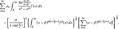
Proof By (9), the reverse of (15), and $0<{\parallel f\parallel }_{p,\tilde{\varphi }}<\mathrm{\infty }$, we have (50). Using the reverse Hölder inequality, we obtain the reverse form of (42) as follows:

$$I\ge J{\parallel a\parallel }_{q,\psi }.$$

(52)

Then by (50), (49) is valid.

On the other hand, if (49) is valid, set $a_n$ as (43), then (44) still holds with $0<p<1$. By (49), we have

$${\parallel a\parallel }_{q,\psi }^q=\sum _{n=1}^{\mathrm{\infty }}{(n-\beta )}^{q(1-\frac{\lambda }{r})-1}{a}_n^q=J^p=I\ge k_{\lambda }(r){\parallel f\parallel }_{p,\tilde{\varphi }}{\parallel a\parallel }_{q,\psi }.$$

(53)

Then by (9), the reverse of (18), and $0<{\parallel f\parallel }_{p,\tilde{\varphi }}<\mathrm{\infty }$, it follows that $J={\{{\sum }_{n=1}^{\mathrm{\infty }}{(n-\beta )}^{q(1-\frac{\lambda }{r})-1}{a}_n^q\}}^{1/p}>0$. If $J=\mathrm{\infty }$, then (50) is trivially valid; if $J<\mathrm{\infty }$, then $0<{\parallel a\parallel }_{q,\psi }=J^{p-1}<\mathrm{\infty }$, i.e., the conditions of applying (49) are fulfilled, and by (53), we still have

$${\parallel a\parallel }_{q,\psi }^q=J^p=I>k_{\lambda }(r){\parallel f\parallel }_{p,\tilde{\varphi }}{\parallel a\parallel }_{q,\psi },\mathit{\text{i.e.}}\text{, }J={\parallel a\parallel }_{q,\psi }^{q-1}>k_{\lambda }(r){\parallel f\parallel }_{p,\tilde{\varphi }}.$$

Hence, (50) is valid, which is equivalent to (49).

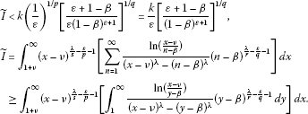
By the reverse of (16), in view of ${\tilde{\omega }}_{\lambda }(x)>k_{\lambda }(r)(1-{\theta }_{\lambda }(x))$ and $q<0$, we have

$$\tilde{L}>k_{\lambda }^{\frac{q-1}{q}}(r)L_1\ge k_{\lambda }^{\frac{q-1}{q}}(r){\{k_{\lambda }(r)\sum _{n=1}^{\mathrm{\infty }}{(n-\beta )}^{q(1-\frac{\lambda }{r})-1}{a}_n^q\}}^{\frac{1}{q}}=k_{\lambda }(r){\parallel a\parallel }_{q,\psi }.$$

Then (51) is valid. By the reverse Hölder inequality again, we have

$$\begin{array}{rcl}I& =& {\int }_{\nu }^{\mathrm{\infty }}\left[\frac{{(x-\nu )}^{\frac{\lambda }{s}-\frac{1}{q}}}{{(1-{\theta }_{\lambda }(x))}^{\frac{1}{p}}}\sum _{n=1}^{\mathrm{\infty }}\frac{ln(\frac{x-\nu }{n-\beta })}{{(x-\nu )}^{\lambda }-{(n-\beta )}^{\lambda }}{a}_n\right]\\ \times [{(1-{\theta }_{\lambda }(x))}^{\frac{1}{p}}{(x-\nu )}^{\frac{1}{q}-\frac{\lambda }{s}}f(x)]dx\ge \tilde{L}{\parallel f\parallel }_{p,\tilde{\varphi }}.\end{array}$$

(54)

Hence, (49) is valid by (51). On the other hand, if (49) is valid, set

$$f(x)=\frac{{(x-\nu )}^{\frac{q\lambda }{s}-1}}{{[1-{\theta }_{\lambda }(x)]}^{q-1}}{\left[\sum _{n=1}^{\mathrm{\infty }}\frac{ln(\frac{x-\nu }{n-\beta })}{{(x-\nu )}^{\lambda }-{(n-\beta )}^{\lambda }}{a}_n\right]}^{q-1}(x\in (\nu ,\mathrm{\infty })).$$

Then by the reverse of (16) and $0<{\parallel a\parallel }_{q,\psi }<\mathrm{\infty }$, it follows that $\tilde{L}={\{{\int }_{\nu }^{\mathrm{\infty }}{[1-{\theta }_{\lambda }(x)]}^{\frac{1}{p}}{(x-\nu )}^{p(1-\frac{\lambda }{s})-1}{f}^p(x)dx\}}^{\frac{1}{q}}={\parallel f\parallel }_{p,\tilde{\varphi }}^{p-1}>0$. If $\tilde{L}=\mathrm{\infty }$, then (51) is trivially valid; if $\tilde{L}<\mathrm{\infty }$, then $0<{\parallel f\parallel }_{p,\tilde{\varphi }}={\tilde{L}}^{q-1}<\mathrm{\infty }$, i.e., the conditions of applying (49) are fulfilled, and we have

$${\parallel f\parallel }_{p,\tilde{\varphi }}^p={\tilde{L}}^q=I>k_{\lambda }(r){\parallel f\parallel }_{p,\tilde{\varphi }}{\parallel a\parallel }_{q,\psi },\mathit{\text{i.e.}}\text{, }\tilde{L}={\parallel f\parallel }_{p,\tilde{\varphi }}^{p-1}>k_{\lambda }(r){\parallel a\parallel }_{q,\psi }.$$

Hence, (51) is valid, which is equivalent to (49). It follows that (49), (50), and (51) are equivalent.

If there exists a positive number $k\ge k_{\lambda }(r)$ such that (49) is still valid as we replace $k_{\lambda }(r)$ by k, then, in particular, (24) is valid. Hence, we have (25). For $\epsilon \to 0^{+}$ in (25), we obtain $k\le \frac{1}{{\lambda }^2}{[B(\frac{1}{s},\frac{1}{r})]}^2=k_{\lambda }(r)$. Hence, $k=k_{\lambda }(r)$ is the best value of (49). We confirm that the constant factor $k_{\lambda }(r)$ in (50) ((51)) is the best possible. Otherwise, we can get a contradiction by (52) ((54)) that the constant factor in (49) is not the best possible. □

Theorem 8 If the assumption of $p>1$ in Theorem  5 is replaced by $p<0$, then the reverses of (39), (40), and (41) are valid and equivalent. Moreover, the same constant factor is the best possible.

Proof In a similar way as in Theorem 7, we can obtain that the reverses of (39), (40), and (41) are valid and equivalent.

If there exists a positive number $k\ge k_{\lambda }(r)$ such that the reverse of (39) is still valid as we replace $k_{\lambda }(r)$ by k, then, in particular, (26) is valid. Hence, we have (27). For $\epsilon \to 0^{+}$ in (27), we obtain $k\le \frac{1}{{\lambda }^2}{[B(\frac{1}{s},\frac{1}{r})]}^2=k_{\lambda }(r)$. Hence, $k=k_{\lambda }(r)$ is the best value of the reverse of (39). We confirm that the constant factor $k_{\lambda }(r)$ in the reverse of (40) ((41)) is the best possible. Otherwise, we can get a contradiction by the reverse of (42) ((46)) that the constant factor in the reverse of (39) is not the best possible. □

Remark 9 (i) For $\beta =\nu =0$ in (39), it follows

(55)

In particular, for $\lambda =1$, $p=q=r=s=2$, (55) reduces to (5).

• (ii) For $\nu =\beta$ in (39), we have

  

  (56)

which is more accurate than (55).

References

Hardy GH, Littlewood JE, Pólya G: Inequalities. Cambridge University Press, Cambridge; 1952.
Yang B: On a more accurate Hardy-Hilbert’s type inequality and its applications. Acta Math. Sin. Chinese Ser. 2006, 49(2):363–368.
Mitrinović DS, Pečarić JE, Fink AM: Inequalities Involving Functions and Their Integrals and Derivatives. Kluwer Academic, Boston; 1991.
Pachpatte BG: On some new inequalities similar to Hilbert’s inequality. J. Math. Anal. Appl. 1998, 226: 166–179. 10.1006/jmaa.1998.6043
Gao M, Yang B: On the extended Hilbert’s inequality. Proc. Am. Math. Soc. 1998, 126(3):751–759. 10.1090/S0002-9939-98-04444-X
Hu K: On Hardy-Littlewood-Polya inequality. Acta Math. Tcientia 2000, 20: 684–687.
Lu Zh: Some new generalizations of Hilbert’s integral inequalities. Indian J. Pure Appl. Math. 2002, 33(5):691–704.
Yang B, Rassias TM: On the way of weight coefficient and research for the Hilbert-type inequalities. Math. Inequal. Appl. 2003, 6(4):625–658.
Kuang J, Debnath L: On new generalizations of Hilbert’s inequality and their applications. J. Math. Anal. Appl. 2000, 245: 248–265. 10.1006/jmaa.2000.6766
Sulaiman WT: On Hardy-Hilbert’s integral inequality. JIPAM. J. Inequal. Pure Appl. Math. 2004., 5(2): Article ID 25
Yang B: An extension of the Hilbert’s type integral inequality and its applications. Journal of Mathematics (PRC) 2007, 27(3):285–290.
Zhong W, Yang B: A reverse Hilbert’s type integral inequality with some parameters and the equivalent forms. Pure Appl. Math. 2008, 24(2):401–407.
Yang B: On a relation to two basic Hilbert-type integral inequalities. Tamkang J. Math. 2009, 40(3):217–223.
Yang B: A strengthened Hardy-Hilbert’s type inequality. Aust. J. Math. Anal. Appl. 2006., 3(2): Article ID 17
Yang B: On a Hilbert-type operator with a symmetric homogeneous kernel of -1-order and applications. J. Inequal. Appl. 2007., 2007: Article ID 47812
Zhong J, Yang B: On a relation to four basic Hilbert-type integral inequalities. Appl. Math. Sci. 2010, 4(19):923–930.
Yang B: A Hilbert-type inequality with the homogeneous kernel of real number-degree and the reverse. Journal of Guangdong Education Institute 2010, 30(5):1–6.
Yang B: A mixed Hilbert-type inequality with a best constant factor. Int. J. Pure Appl. Math. 2005, 20(3):319–328.
Yang B: A half-discrete Hilbert’s inequality. Journal of Guangdong University of Education 2011, 31(3):1–8.
Yang B: On a half-discrete Hilbert-type inequality. Journal of Shantou University (Natural Science) 2011, 26(4):5–10.
Yang B: On a half-discrete reverse Hilbert-type inequality with a non-homogeneous kernel. Journal of Inner Mongolia Normal University (Natural Science Edition) 2011, 40(5):433–436.
Yang B: A half-discrete reverse Hilbert-type inequality with a non-homogeneous kernel. Journal of Hunan Institute of Science and Technology Natural Sciences 2011, 24(3):1–4.
Xie Z, Zeng Z:A new half-discrete Hilbert’s inequality with the homogeneous kernel of degree . Journal of Zhanjiang Normal College 2011, 32(6):13–19.
Yang B: A new half-discrete Mulholland-type inequality with parameters. Ann. Funct. Anal. 2012, 3(1):142–150.
Chen Q, Yang B: On a more accurate half-discrete Mulholland’s inequality and an extension. J. Inequal. Appl. 2012., 2012: Article ID 70. doi:10.1186/1029–242X-2012–70
Zhong W: A mixed Hilbert-type inequality and its equivalent forms. Journal of Guangdong University of Education 2011, 31(5):18–22.
Yang B: the Norm of Operator and Hilbert-Type Inequalities. Science Press, Beijing; 2009.
Kuang J: Applied Inequalities. Shandong Science Technic Press, Jinan; 2010.
Kuang J: Real and Functional Analysis. Higher Education Press, Beijing; 2002.
Kuang J: Introduction to Real Analysis. Hunan Education Press, Changsha; 1996.
Acknowledgements
This work is supported by the Emphases Natural Science Foundation of Guangdong Institution, Higher Learning, College and University (No. 05Z026), and Guangdong Natural Science Foundation (No. 7004344).
Author information
Authors and Affiliations
Corresponding author
Additional information
Competing interests
The authors declare that they have no competing interests.
Authors’ contributions
AW carried out the study, and wrote the manuscript. BY participated in its design and coordination. All authors read and approved the final manuscript.
Rights and permissions
Open Access This article is distributed under the terms of the Creative Commons Attribution 2.0 International License (https://creativecommons.org/licenses/by/2.0), which permits unrestricted use, distribution, and reproduction in any medium, provided the original work is properly cited.
About this article
Cite this article
Wang, A., Yang, B. A new more accurate half-discrete Hilbert-type inequality. J Inequal Appl 2012, 260 (2012). https://doi.org/10.1186/1029-242X-2012-260
Received:
Accepted:
Published:
DOI: https://doi.org/10.1186/1029-242X-2012-260