
Abstract
Driven by advances in miniaturized electronics, many robotic systems today consist of modular hardware components. This leads to numerous computing units that are distributed within such systems. In order to make better use of such hardware structures from a computational point of view, the implementation of classical control approaches should be reconsidered. Following this idea, a method for distributed computation of motion dynamics of robotic systems using Field Programmable Gate Arrays is discussed. In this approach, local low-level actuator controllers are regarded as interconnected nodes, which are aware of their actuated degree of freedom and the resulting motion of the attached rigid body link element. A modified recursive Newton–Euler algorithm is computed by these nodes, where each node only exchanges data with the neighboring nodes. In the computations, a linear dependency on the dynamic parameters is kept in order to simplify the direct use of dynamic parameters estimated from experimental data. Implementation details and experimental results using a robotic manipulator arm are presented. The experiments show that the method allows compliant motion control. Payloads and external forces acting on a link are considered in the distributed computation of the model by informing the node controlling the respective link of the additional forces.
1 Introduction
While it is still common for heavy industrial robotic systems with a large control cabinet to do the actuator control in a central system, it has become unfavorable for lightweight systems as used for human–robot collaboration or mobile systems. In particular, availability of micro-controllers and miniaturized power electronics has advanced greatly in the recent decades, while at the same time costs have dropped. Instead of routing every motor’s power lines and every sensors connection through the structure to a central control system, local control loops computed by the electronics placed at each actuator are used. Consequently, a shared communication bus and a power supply line routed through the structure are sufficient. These increasing local computational capabilities and decision logic motivate researching distributed control approaches and even question the centralized computation of classical algorithms. One aspect is to make better use of the hardware structure. However, using decentralized control techniques has a number of additional advantages, such as simplification of the controller design problem, lower latencies in local control loops, and support of modularity.
In this work, the focus is on the distributed computation of motion dynamics of a robotic system. A model of the robot motion dynamics is the basis for many advanced motion and force control approaches. Classically, it is computed centrally in a fixed control cycle. Such model relates the actuation forces or torques with the motion of the system and external forces and is therefore fundamental for advanced motion and force control of robotic systems. However, since these models depend on the state of all degrees of freedom, the common approach is to obtain the complete state of each actuator, compute centrally the control loop including the motion dynamic model, and send an updated motor command to each actuator. This means, all the state and sensory information has to be messaged from the distributed units to a central point prior to computation of the control update. After the update, the new commands are messaged to the actuators in return. This synchronizes the control actions to a frequency constrained on one hand by the requirement to be computed online and on the other hand by response time and thus control stability. A solution to this problem applied in industrial robot manipulators is to use a communication system specifically tailored to the complete system in order to meet the requirements of control frequency and latency.
However, this approach does not scale well to robotic systems which become more modular, more complex in terms of number of degrees of freedom (DOFs), types of actuators, and increasing amount of sensory information coming from hardware distributed all over the system. For these applications, a central control approach becomes difficult to design in terms of complexity and reaction time. Using local control loops can help to reduce the design effort and support modularity.
1.1 Related work
Creating models and control systems in a distributed fashion is a principle being studied in many technical areas, and similar principles can also be found in the non-technical domain. In political systems, for instance, this is known as subsidiarity, “the principle that a central authority should have a subsidiary function, performing only those tasks which cannot be performed effectively at a more immediate or local level” [28]. From the perspective of the technical domain, there are some potential advantages:
- (1)
It can be simpler and a more structured approach to define smaller models and interconnecting them than dealing with complex, monolithic models. This can be exploited in modeling of multi-body physical systems. For instance, Eberhard et. al. discuss hierarchical modeling approaches [18]. Also, the structure of multi-body systems can be exploited to parallelize the forward dynamics computation in order to simulate the system behavior more efficiently [17]. In robotics, decomposition of complex problems into smaller subproblems of lower dimensional space is a traditional approach, for instance, introduced by Brooks [11] and extended later for behavior-based control [2] in the area of behavior-based systems. These design principles aim to reduce the complexity of the tasks and allow to build a complex controller incrementally. Similarly, in the area of reinforcement learning, there exist approaches such as hierarchical reinforcement learning, which is based on decomposing the robot’s task, either manually or automatically, into a hierarchy of subtasks [9], being motivated by the fact that standard reinforcement learning would poorly scale with large state spaces.
- (2)
Subsequently, it can help to reduce the controller design effort. D’Andrea et. al [15] discuss the control of interconnected systems, in particular systems, which “consist of similar units which directly interact with their nearest neighbors.” For such kind of systems, the authors argue against centralized control schemes, as “It is also not feasible to control these systems with centralized schemes—the typical outcome of most optimal control design techniques—as these require high levels of connectivity, impose a substantial computational burden, and are typically more sensitive to failures and modeling errors than decentralized schemes.” Similarly, Massioni et. al. argue for investigation of decentralized or distributed controller architectures for large scale systems and present a procedure for “simplifying the computational complexity of the problem as well as for finding a controller with a distributed architecture” [25].
- (3)
Latencies can be reduced within actual implementations by parallelization or distribution of the computations in hardware. In [29], Paine et. al. discuss an actuator-level control approach. The aspect of distributed computation is focused on decoupling the actuator dynamics of serial elastic actuators form the link dynamics. This is reasonable, as on the one hand the system boundaries of the dynamics of one actuator can be chosen such that the actuator dynamics are not directly dependent on the other actuators’ states. And on the other hand, it is highly beneficial for the responsiveness of the serial elastic actuators, because latencies are reduced and control frequencies can be increased in dedicated local controllers. Similarly, Zhao et. al motivate the use of distributed controllers, particularly in view of the computational and communication requirements of complex human-centered robotics. In [48], the authors study the stability and performance of distributed controllers, where stiffness and damping servos are implemented in distinct processors. As experimental evaluation, an operational space controller is implemented in a mobile base. A combination of these two studies can be found in [49].
Using implementations based on Field Programmable Gate Arrays (FPGAs) is particularly interesting for motion control applications, because they allow high sampling rates and a very flexible programming of parallel tasks. For example, in [47] Shao & Sun describe a motion control system using a FPGA for computation of servo control loops. Regarding the particular algorithm used for the computation of the dynamics in the work presented here, in an early work [33] Rajagopalan discusses the computational viewpoint in a parallel computation setup. The author describes a partitioning approach of the Newton–Euler algorithm, such that a parallel computation on multiple transputers is enabled. The focus is solely put on the parallel computation of the dynamic model in order to reduce the computation times, in contrast to viewing actuator controllers as nodes interconnected to each other. The approach significantly reduces computation time by using parallel computation on transputer processors. While nowadays a usual office computer will suffice for computing a 6-DOF rigid body dynamic model sufficiently fast, the complexity of robotic systems in terms of number of DOFs and model complexity increased in the meantime as well. It is therefore reasonable to continue to research methods which allow to scale with this trend.
- (4)
Furthermore, some systems such as robots within a swarm require distributed control approaches, because these individual units need to function autonomously and still achieve common goals by interacting with each other. In fact, the distinction of complex robotic systems to swarm robotics narrows down to the mechanical connection of the links. However, a growing number of “smart” actuators, grippers, sensors, platforms, and other modules used to build up robotic systems highly adapted to the target purpose in a modular way blur this distinction. These systems can also be mechanically reconfigurable at runtime, such as the modular robotic platform shown in Fig. 1 [10, 37]. And on the other hand, there are swarm robots which do in fact connect mechanically in order to achieve a common manipulation or locomotion goal [7, 22]. For instance, Baele et. al. state:
When it is advantageous to do so, these swarm robots can dynamically aggregate into one or more symbiotic organisms and collectively interact with the physical world via a variety of sensors and actuators.
A robotic system composed of numerous actuators and sensors can be viewed similarly, as this usually involves freely programmable electronic devices distributed all over the system. An example for such kind of systems is shown in Fig. 2; a more detailed description is given by Peters et. al. in [30].
Fig. 1 Fig. 2 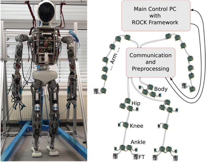
Left: body of the humanoid robot RH5; right: partial view on the structure of the more than 50 freely programmable units distributed across the system


As we can see, distributed computation and control are intensively investigated and in the field of robot motion dynamics development is rather twofold—on the one hand toward modular hardware and, on the other hand, toward parallelization on the algorithmic level.
Contributions The approach presented here advances into the direction of distributed control of a robotic system’s motion dynamics and aims at bringing the two concepts closer together. In particular, the local actuator controllers of a robotic manipulator arm are extended such that a dynamic model of the system is incorporated directly on a local level using a distributed computation of the motion dynamics. This creates a network of interconnected nodes. Each node uses the knowledge of the kinematics and dynamics of its controlled link to propagate the kinematic and dynamic quantities to the mechanically neighboring nodes. For the evaluation, a robotic arm composed of six revolute actuators interconnected by rigid links is used. Each of the arm’s actuators is controlled by a dedicated electronic unit based on a FPGA, which is used to compute the control law using the dynamic model. The distributed dynamics computation enables the system to compliantly react to disturbances while tracking a trajectory, to exert external forces on the environment, and to take payload forces into account.
Paper Organization The next section will describe the derivation of the dynamic model and the algorithm used in this work. On the basis of these results, Sect. 3 describes the approach to distribute the computations, including the implemented software components, and the structure of the implemented actuator controllers. Subsequently, Sect. 4 presents the experimental results of the application using a robotic manipulator arm, which are discussed in Sect. 5. Finally, Sect. 6 discusses the conclusions.
2 Modeling
In order to control the motion of a robotic system in a compliant way based on the actuation torques or forces, it is necessary to know the underlying relationship. For the purpose of motion control of rigid body systems, the most notable formulation is an inverse dynamics model, computing the actuation forces and torques \(\tau (t)\in {\mathbb {R}}^n\) as a function of the motion described in terms of the generalized joint positions \(q \in {\mathbb {R}}^n\), velocities \(\dot{q}\), and accelerations \(\ddot{q}\):
The use of such models allows to compute the feed-forward torques and forces for a reference trajectory, and to decouple the often highly nonlinear dynamics of the robotic system. Consequently, linear feedback controllers with significantly reduced gains can be used, since these only need to compensate for the remaining model-plant mismatch, rather than considering the complete dynamics as error when not using model-based control. With this reduction in feedback, accurate trajectory tracking in an undisturbed case is much less dependent on the controller gains and the feedback controllers can rather be tuned such that a desired compliance wrt. external forces is obtained.
The derivation of equations of motion for rigid body system as well as the development of controllers based on them has been extensively studied and is covered in many classical text books [5, 14, 23, 36]. The most notably used algorithms are the Lagrange method and the recursive Newton–Euler method. The Lagrange method is based on a balance of potential and kinetic energy and, using the classical formulation, from this balance derives the equations of motion explicitly.
On the other hand, the recursive Newton–Euler algorithm is based on the balance of forces and torques. Early work describing the process of modeling the relationship (1) for a robotic system using the Newton–Euler method can be found in [27]. Due to the iterative computation, the algorithm scales much better with the number of degrees of freedom, i.e., with a computational complexity of about \({\mathcal O}(n^{1})\) compared to about \({\mathcal O}(n^{3})\) for the Lagrange formulation [44]. While an iterative reformulation of the Lagrange formulation exists that reduces the complexity to about \({\mathcal O}(n^{1})\), it is not as efficient in terms of the number of multiplications and additions as the recursive Newton–Euler algorithm [21]. In addition, the recursive Newton–Euler algorithm has a structure suitable for a distributed computation and is therefore chosen in this work.
The above-mentioned methods derive the equations of motion from physical insight. However, the numerical values of the parameters contained in these equations are yet unknown. Thus, the model equations are derived in a way such that the unknown dynamic parameters are constant and linearly dependent on the rest of the model. The following sections will describe the algorithm used for the distributed dynamics computation in more detail which is based on the definitions given in [36], with a reformulation as in [1, 6] in order to obtain a linear dependence on the dynamic parameters.
2.1 Recursive Newton–Euler algorithm revisited
Instead of taking the whole system with all its links into account at once, a single link body and its actuated joints are considered as sub-system. For such a sub-system, a balance of forces and torques acting on the \(i-th\) link’s body is derived individually. This balance is described for the forces by Newton’s second law (2), giving the relation to the linear acceleration \(\ddot{p}_{C_i}\) of the center of mass of the body:
where \(f_{i} \in {\mathbb {R}}^{3}\) is the force acting on body i, \(m_i\) is the mass of body i, and \(g_0\) is the vector of gravity acceleration. Additionally, Euler Equation (3) gives us the relation of torques acting on the body and the respective rotational motion:
where \(\mu _{i} \in {\mathbb {R}}^{3}\) is the torque acting on body i, \(\omega _i\) is the angular velocity, \(r_{i,C_i}\) denotes the vector from frame i origin to the body’s center of mass, and \(I_i \in {\mathbb {R}}^{3x3}\) is the inertia tensor of body i,
The dependence on joint states and thus time has been omitted here to improve readability. To take advantage of constant parameters, we further relate Eqs. (2) and (3) to a reference coordinate frame attached to body i. The balance of forces and torques for body i is then given by
where the \({\mathbf {R}}^{i}_{i+1}\) denotes the rotation matrix used to change a vectors reference coordinate system from \(i+1\) to i. Thus, the superscript denotes the reference frame, e.g., \(f^{c}_{b}\) denotes the force vector of body b expressed in coordinate system c. The gravity acceleration has been joined into \(\ddot{p}_{C_i}\). An additional vector \(r^{i}_{i-1,i}\) is introduced, which is the vector pointing from the coordinate system \(i-1\) origin to the origin of coordinate system i. The algorithm solves these two expressions in two steps. In the first step, known as the forward recursion, starting from the base link, the kinematic quantities are calculated iteratively for each body. These are namely the angular velocity as well as the linear and angular acceleration. These quantities depend on the geometry of the kinematic chain, and, depending on the application, each joint state or reference state in terms of joint position \(q_i\), velocity \(\dot{q}_i\), and acceleration \(\ddot{q}_i\). The second step is known as the backward recursion. In this step, starting from the distal link(s), the forces and torques for each body are calculated iteratively according to (5) and (6).
For a revolute joint, the resulting joint or actuation torque can then be computed by projecting the torques acting on the link along the joint’s axis of motion. Using the Denavit–Hartenberg convention, this is the z-axis of the previous body’s coordinate system, \(z^{i-1}_{i-1}\). Thus, the joint torque is given by
A detailed description of the algorithm can be found in [36, p. 283ff].
2.2 Linearity of the dynamic parameters
If the dynamic parameters contained in Eq. (7) are not known beforehand, they can be estimated by means of experiments, also known as parameter identification [8, 42]. For the purpose of simplifying the parameter identification procedure numerically, a notable property of the above equations can be exploited: When referring the terms of the equations of motion to a coordinate system attached to the respective body, the dynamic parameters become independent of the joint configuration and are constant. In fact, the equations can be reordered such that a linear dependency is obtained. The vector of joint torques and forces is then defined by
Note that \({\mathbf {Y}}\) can still contain highly nonlinear terms wrt. the system state. This partitioning and thus the parameter vector \(\pi\) depend on the choice of coordinate systems. Referring the first and second moment of inertia parameters to a coordinate system attached to body i, with its origin and z-axis aligned with the distal joint of the body, the following partitioning of (5) and (6) can be derived when written in matrix-vector form:
The matrix \({\mathbf {T}}^{i}_{W,i+1}\) gives the relation to the wrench transmission of the neighboring body \(i+1\) of the chain on body i, where \({\mathbf {T}}^{i}_{W,i+1}\) is defined as:
The vector \(\pi _i \in {\mathbb {R}}^{10}\) of dynamic parameters for body i, where the inertia tensor \(\bar{{\mathbf {I}}}_{i}\) has been derived from \({\mathbf {I}}_i\) by referring it to the origin of the attached coordinate frame according to the parallel axis theorem, is determined as
The choice of parameter vector (11) was also influenced owing to compatibility wrt. a previously used implementation based on the Lagrange formalism and thus to allow for comparison and reusing previously estimated parameters (further details are given in Appendix). The corresponding matrix \({\mathbf {W}}_i \in {\mathbb {R}}^{6\times 10}\) is given by Eq. (12) using the following definitions:
and
such that the relation \({\mathbf {I}} \omega = {\mathbf {L}}(\omega ) \left( {\mathbf {I}}_{xx}, {\mathbf {I}}_{xy}, {\mathbf {I}}_{xz}, {\mathbf {I}}_{yy}, {\mathbf {I}}_{yz}, {\mathbf {I}}_{zz} \right) ^T\) holds.
By concatenation, the vector of all dynamic parameters \(\pi = \left( \pi _1^T,\ldots ,\pi _n^T \right) ^T\) is obtained. Looking at the complete chain of interconnected bodies, an expression for all the wrench vectors stacked, e.g.,
is obtained with the matrix \({\mathbf {W}}\) of the form
External forces acting on a body can be taken into account here by addition in (9). In this case, the structure of the matrix \({\mathbf {W}}(q, \dot{q}, \ddot{q})\) can be kept by adding the external wrench into additional columns and extension of the parameter vector \(\pi\) by 1-elements.
Tree structures In case, body i has more than one consecutive body, e.g., a tree-structured mechanism, we can apply the algorithm similarly. Firstly, the forward recursion is computed for every following kinematic chain, e.g., for every branch. In the backward recursion, the wrenches of every of the branches are added in (9), such that for every consecutive body (child) \(C_1 \ldots C_j\) a term is appended:
The parameter vector has to be adapted accordingly, in the same order as the added columns of \({\mathbf {W}}\). Equally as in (7), the projection on the motion axis for a revolute joint can be rewritten as:
where \({\mathbf {W}}_{\mu ,i}\) refers to the lower 3 rows of the matrix \({\mathbf {W}}_{i}\).
To summarize, the dynamic parameters are separated from the rest of the model and a linear relation has been obtained as defined in (8).
2.3 External forces and compliance
The mapping from an external force or torque \(F_{ext}\) acting on the system structure to the actuation forces and torques is given by
where \({\mathbf {J(q)}}\) denotes the Jacobian wrt. the contact point and has to be evaluated for the joint configuration q. Different measures exist to characterize the velocity and force manipulability in the workspace of the system by analyzing the properties of the Jacobian matrix. In the event of reaching a singular configuration, this results in reduction in the matrix rank of \({\mathbf {J(q)^T}}\), and in practice, configurations in which this matrix becomes ill-conditioned pose a problem as well [35, Sec. 1.10, 11.2.2, 29.5].
Mechanically this can mean, for example, some elements of an external force vector are solely supported by the structure and cannot be influenced by the actuation forces. In such case, the ability of the system to react compliantly to such external forces in the respective direction is lost. Equivalently, when reaching the mechanical limit of a joint, a further compliant reaction in the respective work space direction is only possible using the remaining degrees of freedom. This is a general limitation of compliant control schemes based on the compliance in the actuation system, since the work space has to be mapped to the available joint space. The problem can be mitigated by providing a sufficient number of DOFs or additional flexibilities in the structure, by planning trajectories which avoid coming close to singular configurations, or even covering the whole structure with soft materials.
2.4 Friction
For robotic actuators, often using gear reduction mechanisms, friction can become a significant fraction of the joint torque or force. If the torques or forces are measured directly at the output shaft, the joint and gear friction can be compensated for easily, i.e., by an additional feedback loop controlling the torque at the output shaft. However, often this measurement is not available such as in the case presented in Sect. 4. In this case, a friction model is required to estimate the additional motor torque or even motor current required for a compensation. Several friction models are available. A first—in many cases sufficient—approximation is to introduce Coulomb and viscous friction terms such as \(\tau _{c,i}(t) = F_{C,i}\, sign(\dot{q}_i(t))\) and \(\tau _{v,i}(t) = F_{v,i}\, \dot{q}_i(t)\), respectively. To avoid numerical problems, it is reasonable to replace the signum function by a function fulfilling the Lipschitz continuity condition, such as \(atan(k\cdot \dot{q})\). The design parameter k allows to control the steepness around zero velocity. Most often friction parameters can be estimated with the other dynamic parameters simultaneously. Additionally, a measurement offset \(b_i\) can be necessary in practice, which can as well be estimated as part of the identification procedure. Keeping the parameters separate, the model for the friction torque \(\tau _{F,i}(t)\) of a rotational joint i can be summarized as
Using more complicated friction models such as Stribeck friction models (see, e.g., [24]) usually requires a preliminary, separate identification per actuator, or training in case of using machine learning approaches, in order to properly distinguish friction effects from other effects. In this case, a separate identification helps to avoid overfitting, e.g., undesired mapping of friction parameters onto other effects, and to avoid introduction of further states such as temperature into the identification procedure carried out for the mass and inertia parameters. Further discussion of friction effects from the perspective of control can be found in [4].
2.5 Identification of the dynamic parameters
While the forward recursion is only dependent on the kinematic information of the system, i.e., the link geometries and joint DOFs, the backward recursion depends on the dynamic parameters for each body of the system. Usually geometric information is accurately available from CAD data or can be obtained by direct measurement. Dynamic properties on the other hand are often only very approximately available from CAD data. For instance, the mass distribution of more complex parts bought from external suppliers could be inaccurately known, and others, such as wires, are hard to approximate. An alternative is provided by experimental identification: A high-gain joint controller is used to track a reference trajectory, while the motion and the generated actuation torques and forces, which were necessary, are measured. Using the previously derived model, the dynamic parameters can be estimated from the measurement data. Note that not all dynamic effects have an influence on the joint torque, but will be transmitted directly by the structure, or those effects are indistinguishable from each other. Therefore, a reduction of the dynamic parameter vector can be performed. This means to identify the linear combinations and unidentifiable parameters, either by rules or numerically by inspecting a regression matrix based on \({\mathbf {Y}}\left( q,\dot{q}, \ddot{q}\right)\). Figure 3 gives an overview of an exemplary procedure from the initial theoretical modeling of the robot motion dynamics to a model having experimentally identified parameters.

Tasks and data flow used to model and identify robot dynamics experimentally
In more detail, this type of classical identification procedure usually includes the following main steps.
The first step is to derive the system’s equations of motion from physical insight as discussed in Sect. 2.1. With this prior information, the second step is to design experiments, which will be used to generate the measurement data. To reduce the experimental effort and to obtain useful rich measurement data, a reference trajectory in joint space can be optimized to maximize the expected richness wrt. the informational content of the resulting measurement. Assuming a trajectory sampled at K points in time with sampling period \(T_s\), evaluating (8) for each sampled set of joint motion, we obtain a concatenated matrix for the complete trajectory:
The equation to be solved by estimating the parameter vector \(\hat{\pi }\) is then given by
where \(\tau _{msr} \in {\mathbb {R}}^{Kn}\) is the concatenated vector of measured joint torques or forces. A practical method to find a trajectory such that \(\hat{\pi }\) can be optimally estimated within the robot constraints is described by Swevers et. al. in [41, 42]. It uses Fourier series as fundamental functions to generate the joint trajectories, which determine \(q(kT_s)\): Specifically, the trajectories are based on the Fourier series function
which determines the joint angles \(q_i(t)\) for each joint i as function of the Fourier coefficients \(q_{i,0}\), \(a_{i,h}\), and \(b_{i,h}\). This results in smooth excitation trajectories, whose frequency spectrum is band limited by the choice of \(\omega _f\) and the number of harmonics \(n_{harm}\) and thus allows to avoid excitation of unmodeled effects having higher resonant frequencies. Joint velocities \(\dot{q}_i(t)\) and accelerations \(\ddot{q}_i(t)\) can be computed by analytical differentiation of (23), which is especially useful to avoid a numerical differentiation for the second derivative \(\ddot{q}\). The Fourier coefficients are optimized using the d-optimality criterion as measure for the information content [39]. A number of alternate methods can be found in the literature, which mainly differ in the way the trajectory is parameterized and the criteria used for the optimization (see, e.g., [3, 19, 31, 32, 40]). With the computational power available today, the algorithm efficiency is not as critical as some decades ago, therefore greatly simplifying the implementation of an optimization routine.
The optimization is subject to a number of constraints. In particular, joint limits such as joint motion ranges, velocity limits, and acceleration limits have to be fulfilled. In addition, limits in the Cartesian workspace are necessary to avoid collisions with the environment. In this work, a set of box constraints have been imposed on the coordinate origins of the last two links of a 6-DOF manipulator arm, such that the z-coordinate constraints prevent collisions with the table on which the arm is mounted on. In an iterative procedure, it is also possible to include approximate limits on the required joint torques. Based on (23) and using the d-optimality criterion as measure of information content, the optimization problem is as follows:
Here \(\varPhi\) has been reduced to a matrix \(\bar{\varPhi }\) having full matrix rank by removing columns not contributing to the rank and merging columns of linear combinations.
The third step is then to carry out the experiments and to obtain the measurement data, namely the measured actuation torques or forces \(\tau _{msr}\) as well as the measured joint positions. Eventually—and often in case of prototype robotic systems—the experimental results indicate a decrease or increase in the constraints used for the experiment optimization. In such case, a number of iterations are necessary to find suitable values. This equally applies to the fundamental frequency \(\omega _f\) and the number of harmonics \(n_{harm}\).
Finally, using the obtained measurement data, the last step is to estimate the dynamic parameters. On the basis of (22), a linear estimation problem has to be solved. Without further constraints, a simple least squares estimator can be used. However, it is reasonable to also impose constraints on the estimation problem, in order to ensure physical consistency of the model parameters such as positive mass parameters and positive definite inertia tensors. Thus, the parameter vector is estimated by
subject to the physical consistency constraints (see, e.g., [43, 46]).
3 Distributed dynamics computation
Let us consider a chain of rigid bodies interconnected by rotational joints as is the case for the robotic arm shown in Fig. 8. Each of the rotational joints is actively actuated, and each actuator is controlled by a dedicated stack of electronics as shown in Fig. 4.

SpaceClimber robotic actuator and FPGA electronics [20]
The structure of the algorithm presented in the previous section is mapped onto these computational units. In particular, each actuator controller has to carry out the same computations using the inputs provided by the neighboring actuator controllers and the state of the controlled joint itself. The operations to be carried out are summarized in Fig. 5.

Operations to be carried out by each actuator controller in order to compute the inverse dynamics. Left connections to proximal neighbor, right connections to distal neighbor. Top and bottom connections: local state (or reference) variables and configuration variables (dashed)
For the first actuator controller, the kinematic quantities such as the angular velocity, the linear and angular acceleration are configured as constants or supplied by the central controller, e.g., in case of a moving base. The first actuator controller then calculates the resulting motion taking into account the actuator motion and the geometry of the connected body. This information is provided to the next adjacent actuator controller. This procedure continues until the actuator controller of the most distal link is reached, which does not have any further neighbors. It initiates the backward recursion, by calculating the wrench vector and transmitting this information to the previous proximal controller. When the first actuator controller has calculated its wrench vector, the computation is finished and every controller knows the required torque for the actuator as computed by the model.
This whole procedure can be carried out periodically and at a high frequency, e.g., in the kHz range. Only little information needs to be exchanged, in particular only between directly neighboring actuator controllers. In this way, a centralized controller is relieved from the time-critical tasks to read all the joint states, to compute the complete inverse dynamics model, and to write the updated torque or force information back to every actuator controller. The following update policies are generally feasible: 1) sequential update of the actuator controllers, 2) parallel updates, i.e., each actuator controller computes the update and informs the neighboring controllers simultaneously, and 3) internal loop runs faster than complete chain update, i.e., the local controllers transiently update using the local state obtained from local sensor information more often than exchanging the state updates with the neighboring actuator controllers.
3.1 Implementation
Each actuator is controlled by a stack of electronics (Fig. 4) which is equipped with a FPGA for the computations and signal processing. This is the third of multiple generations of these FPGA-based actuator electronics, which have been developed for use in various robotic systems. The advantages of using a FPGA-based approach are the ability for inherent parallel processing capabilities and the perspective to switch to radiation tolerant devices [38].
Central/PC Implementation Initially, the model equations have been implemented as a C-library. It allows to compute the inverse dynamics model for central control methods and is used for the identification procedure as well as for simulation purposes. Additional software libraries and scripts have been developed for the identification to solve the tasks shown in Fig. 3. The central controller uses the component-based software framework ROCK [34] to communicate with the hardware, to generate the reference trajectory, and to log the measurement data.
FPGA LinkDyn Component In order to compute the dynamics according to Fig. 5 on FPGAs, a component named LinkDyn has been programmed using VHDL. The component is composed of modules as shown in Fig. 6.

Internals of the implemented VHDL component LinkDyn to compute the dynamics of a single node on a FPGA
This module expects the following inputs: sine and cosine of the Denavit–Hartenberg (DH) parameter \(\alpha\), the DH parameters a, d, and \(\vartheta\), and the state or reference of the controlled actuator in terms of \(q_i\), \(\dot{q}_i\), \(\ddot{q}_i\). As output, the computed torque is provided. All other quantities such as the linear acceleration, angular acceleration, and velocity of the proximal neighboring body are exchanged via a shared memory (block ram) interface. Triggers and acknowledge signals are used to start the forward or backward computation.
The main process of the component consists of a number of sub-routines. In addition to the two sub-routines for the forward and backward dynamics computation itself, these are matrix-vector multiplication, cross product calculation, and handling of reading and writing requests from the interface. Matrix-vector multiplication and cross product calculation are a shared routine for all the steps required for the dynamics computation. These are only triggered internally and take precedence over all other sub-routines. Also, a running dynamics computation will not be interrupted, but postpone additional requests. The sine and cosine terms are calculated using a look-up table approach, as the target FPGA (Xilinx Spartan 6) provides sufficient block ram resources. By mirroring and inverting, only \(\frac{1}{4}\)th of a sine period has to be stored. Alternatively, algorithms such as the CORDIC (Coordinate Rotation Digital Computer) or a polynomial approximation can be used. For all variables, a 32-bit fixed-point representations is used. It has been validated by simulation that for a setup as the one used here the differences to using floating point representations are insignificant.
Actuator Controllers Each actuator controller is structured as shown in Fig. 7. At the innermost position, a current controller controls the actuator’s motor current by using pulse width modulation (PWM). The reference current is mainly computed from the local dynamics model and a friction compensation. Additionally, a cascade of high-gain feedback controllers are used. If no limitations of position range and maximum velocity are violated, the output of these controllers is highly limited (e.g., to 3–5% of the nominal current). On the one hand, these controllers mainly have a guarding function and can switch to a higher output, in order to keep the actuator state within the configured limits. On the other hand, the tracking performance in the presence of small model-plant mismatches can be improved due to the high gain and integral action of the controller cascade.
The reference of the model computation is selectable (see block State MUX), either using the actual measured state or using a reference state. As in a classical computed torque control scheme, the input to the model has an additional parallel implementation of a position and velocity feedback controller (blocks \({\mathbf {K_p}}\), \({\mathbf {K_d}}\)). Therefore, the reaction to disturbances can be configured assuming a second-order system, in analogy to a mass–spring–damper system. These controllers, which provide the input to the dynamics model computation, i.e., the linearized and decoupled system, are limited individually. This way, the reference torque is restricted to sensible ranges, under the condition that the reference trajectory is feasible and the dynamic parameters are physically consistent. On the lowest level in the control loop, the actuation torques are limited by the motor current controller to the permissible range. In effect, the implemented approach provides multiple layers within the control architecture which deal with the limitation of actuation torques/forces. As a last resort, the system will also deactivate based on comparing the system state to maximum thresholds. This provides the basic functionality of a compliant manipulator to a higher-level robot control architecture, which can then react—possibly in a larger time frame—to deviations and, for instance, re-plan the reference trajectory in order to avoid an obstacle.

Structure of the joint-level control loop including the dynamics model implemented on a FPGA
Data Exchange Figure 8 shows exemplarily the communication for the COMPI manipulator arm. Initially, the base actuator controller (at J1) receives the base accelerations from the central control PC, computes the forward recursion (yellow blocks) based on the link’s geometry and joint state, and sends the result to the next actuator controller (at J2). Instead of further propagation of the kinematic quantities, the most distal actuator controller (J6) will start the backwards recursion (green blocks) by computing the wrench, using the dynamic parameters of the link it controls. The base actuator controller will complete the backward recursion by sending the computed base wrench to the central control PC. This procedure has been implemented for a frequency of 1kHz.

Left: COMPI manipulator arm (initially without cover). Right: communication procedure of the distributed dynamics computation is shown exemplarily for the system
4 Experimental results
Using the 6-DOF COMPI manipulator arm (Fig. 8), experiments have been carried out to evaluate different aspects of a compliant control scheme based on the distributed computation of the dynamics according to the proposed method. In particular, to evaluate incrementally the distributed dynamics computation within the control scheme, the evaluation starts in a static contact case and subsequently advances to position control at a static reference, compliant control when tracking a Cartesian space trajectory and handling an additional force exerted by a payload. These experiments are described in more detail in the following paragraphs.
4.1 Parameter identification
Since for all of the following control experiments the basis is a model of the motion dynamics of the test system, this section gives an overview of the application of the methods described in Sect. 2.5 for an experimental identification of the system.
The model of the 6-DOF manipulator arm contains 10 dynamic parameters per link and thus a parameter vector of 60 parameters. However, a further inspection reveals unidentifiable parameters and linear combinations, resulting in a reduction of the full parameter vector from 60 parameters to a set of 36 combined parameters.
Using this prior model, the experiment optimization has been carried out with the number of harmonics \(n_{harm}=5\), the fundamental frequency \(\omega _f=0.1s\), and a period \(T_p=10s\). The trajectory and the measurement data are sampled with a period of \(T_s=1ms\). The joint limits used as constraints in the optimization problem are given in Table 1. In addition, the coordinate origin of the 5th and 6th (last) link has been constrained to a minimum height of 0.25m to avoid a collision with the table the arm is mounted on.
The experiments have been carried out then using high-gain position feedback controllers of the actuators in order to closely follow the desired trajectory. To avoid using any further interpolation techniques in these measurements, one period of fade-in and fade-out between the actual trajectory and the initial position of the robot arm is prepended and appended, respectively, to allow for a smooth start and stop. This results in a joint trajectory of similar type as the one shown in Fig. 9. Except the 10 sec of fade-in and fade-out each, only one period is shown here. However, it is reasonable to measure a multiple of periods and to average the measured torques to reduce random measurement noise.
With the measurement data of the actual motion and the corresponding torques generated by the actuators, the parameters have been estimated according to Eq. (25). Prior to the estimation, the model has been extended with a friction model as described in Eq. (20), adding 3 parameters to be estimated per actuator for the friction effects. Including the coefficient k, controlling the steepness of the Coulomb friction term, in the minimization problem, or using more complex friction models did not significantly improve the estimation result in this case. Thus, a fixed value of \(k=100\) has been used. Since the manipulator arm uses a mechanical spring to support the second actuator, the forces generated by the spring have been computed according to the spring constant and the deflection and then added to the second actuator’s torque measurement.
Finally, a validation of the model is shown in Fig. 10. The validation is based on the measured torques when tracking an eight-shaped Cartesian space trajectory, also used for the compliance tests described in Sect. 4.4. The comparison shows that the model-computed torques are predominantly in good agreement with the measured torques, such that the model can be used for the further developments.

Exemplary identification trajectory for a single joint resulting from the experiment optimization based on Fourier series. One period (10s) to fade-in from the initial position has been prepended, and one period to fade-out to the final position has been appended

Results from a validation experiment based on a Cartesian space trajectory; comparison of measured torques and torques computed by the model using the estimated parameters
4.2 Static contact force
As a first test, a setup as shown in Fig. 11 has been used. In this scenario, the gripper holds a screw driver, which is pushed against a fixed board. Accelerations and velocities are therefore zero (neglecting elastic effects), and we can exclude effects such as the second moment of inertia and most friction effects. Moreover, the reference position is chosen such that the initial force is near zero, and the influence of the position and velocity controllers can be neglected as well. Thus, the focus is on two aspects: the forward recursion, testing the kinematic transformations, and the distributed propagation of the external force of the last link, including the gripper, from the last node to the remaining nodes.

Experimental setup used in the static contact force experiment using COMPI manipulator
By setting a nonzero force vector in the last actuator controller’s registers, the model will include this information in the model computation. Consequently, all actuator controllers generate the necessary joint torques, creating the requested force. Since the manipulator is in contact, we can measure the generated force exerted on the board using the 6-DoF force/torque sensor at the wrist as a ground truth. In Fig. 12, the commanded and measured force is shown. The commanded force is generated by a sinusoidal signal of 40N in x direction (horizontal). The measured data show that the force in x direction resembles the commanded force, but saturates at ca. 30N. In addition, an influence on the measured force in z direction is visible. This can result from kinematic inaccuracies, i.e., non-orthogonal orientation of the gripper or the grasped screw driver wrt. the board. Also, elastic effects were visible during the experiment, in particular a bending of the board. The amplitude of the commanded force has been chosen to approximately cover the full range considering the nominal torque of the actuators (28Nm). A model-plant mismatch due to additional effects such as static friction would reduce the available torque and thus leads to a saturation of the generated force. In view of these effects and, in particular, taking into account the fact of controlling the generated torque via the motor currents, the measured force is still in good agreement with the open-loop commanded reference force and well within the range of expectable results.

End-effector forces generated using the open-loop model computation on the COMPI manipulator
4.3 Point control
In a second experiment, compliant control at a static reference joint position has been evaluated. The focus in this test was to determine the reaction of the system to disturbance forces applied to the end-effector. The experiment has been carried out for different settings of the controller gains \(K_p\) and \(K_d\) of the position and velocity feedback controllers, respectively. The outputs of these controllers are added to the joint reference acceleration which is fed into the model computation. This means a control error in one joint state can influence the control action at the other actuator controllers, as the model decouples joint accelerations wrt. the actuator torques. For three different settings—high damping, medium damping, and low damping—of the \(K_p\) and \(K_d\) parameters of the actuator controllers, the reaction to disturbances is shown in Fig. 13. The measurements show that the changes in the controller parameters have the intended effect, e.g., in case of a high \(K_d\) value the system’s reaction wrt. the position is much higher damped than for a low value of \(K_d\), where some periods of a damped oscillation become visible.

Cartesian position error of the end-effector of the COMPI manipulator for different controller gains when disturbed by an external force
4.4 Trajectory tracking and compliance
Extending the previous experiment, in this experiment the manipulator arm tracks a trajectory in the Cartesian work space, while an external disturbance force is applied. The reference trajectory is defined by a Lissajous figure, resulting in an eight-shaped trajectory as shown in Fig. 15. For the joint space control used here, the inverse kinematics are solved centrally in order to obtain the reference joint positions, joint velocities, and joint accelerations. The purpose of this experiment is to evaluate the complete distributed controller setup, where especially the compliant reaction to disturbances is focused. The experimental setup is shown in Fig. 14.

Experimental setup (top) and deflection from reference path wrt. a disturbance force vector (bottom)
As ground truth, the end-effector force sensor is used again. This allows to measure the forces and map them to the positional displacement in order to get a quantitative information of the compliance. The experiment shows that the manipulator arm reacts compliantly to disturbances at the end-effector but also at any other link of the arm, while tracking the reference trajectory. A high compliance, e.g., low feedback gains, has been set. Thus, the arm reacts rather soft to disturbances. In Cartesian space, the end-effector compliance in this joint configuration results in a value of about 10 N / 0.25 m (Fig. 17). However, in case of large deviations from the reference trajectory, e.g., due to contact, the feedback would lead to undesirable high contact forces. It is therefore reasonable to additionally limit the outputs of the feedback controllers, thereby implicitly saturating the contact forces. The manipulator will thus give in to a disturbance above this saturation and move back without further increasing the forces. This is an important feature in the field of human–robot collaboration, where contact forces must not grow indefinitely, and even large deviations from the reference trajectory should be tolerated by the system for forces exerted by a human operator.
Nonetheless, the experiment showed that when using such additional saturations, the robot manipulator is still able to recover immediately from large disturbances and keeps tracking the trajectory accurately, e.g., comparable to using high-gain position controllers. On the other hand, if additional external forces are actually desired, the model should reflect that information as shown in the next section.

Cartesian reference (solid) and measured position (dashed) of the end-effector of the COMPI manipulator when disturbed while moving along a reference trajectory without payload. Time indicated by arrows at every second

Cartesian reference (solid) and measured position (dashed) of the end-effector of the COMPI manipulator when disturbed while moving along a reference trajectory with payload. Time indicated by arrows at every second

Cartesian position error and applied disturbance force during the tracking experiment without payload

Cartesian position error and applied disturbance force during the tracking experiment with payload
4.5 Payload
Instead of considering the external force as a disturbance resulting in a deviation from the reference trajectory due to the compliance, in this experiment, the external force is to be compensated for such that the reference trajectory is tracked closely while the force is applied. Thus, this is a test if an additional force is correctly considered in the model computation, provided the respective actuator controller node is informed about this additional force acting on the link it controls. However, further forces should still result in compliant reaction of the manipulator arm.

Degradation of the tracking performance due to an unmodeled payload with a mass of 0.8kg
For this purpose, the previous experiment is carried out again, but with a payload added to the gripper. The payload is part of a car transmission and has a mass of approximately 0.8 kg. Without further modeling, the trajectory tracking accuracy is degraded due to the low feedback gains. In fact, in this setting the manipulator arm is not at all able to carry the weight as shown in Fig. 19, which results in a severe deviation of, e.g., more than 0.75m in end-effector height. This is the expected reaction, as again a high compliance has been configured, and therefore, the feedback control loops are not capable to compensate for such model-plant mismatch.
However, by informing the last actuator controller of the gravity force introduced by the weight added to its connected link, i.e., the gripper, the tracking accuracy is improved again to the original level as in the tracking experiment without payload, while the system still reacts compliantly to external disturbances (Figs. 16 and 18).
5 Discussion
The purpose of this study was to reconsider the implementation of a classical control algorithm to make better use of the modular hardware modern robotic systems are composed of. In particular, the results show the feasibility to distributedly compute an inverse dynamics model—which usually is a function of all joint states—by partitioning the algorithm to match a robotic system’s modular hardware structure. Thus, this work extends the approach used in [29] where actuator-level dynamics are handled locally; here, also the highly coupled model of rigid-body dynamics is computed locally by allowing the distributed nodes to communicate with their neighboring nodes.
From the computational perspective, the results show that using FPGA-based electronics to compute such kind of model computations is possible with reasonable effort and that it is a benefit since model computation, controllers, communication, motor commutation, and sensor processing are handled in parallel. On the one hand, this extends the work described in [47], where a single FPGA is used for the linear servo control loops only, while additionally a digital signal processor (DSP) is still used to carry out the nonlinear model computations at a lower sampling rate. On the other hand, this can be viewed as an adaption of the approach in [33] to achieve a distribution better suited to the hardware of a robotic system, i.e., allowing for boundaries around each actuator/link pair.
The presented result also shows the arrangement of the model equations such that a linear dependency of the dynamic parameters is kept in the distributed computation. This is beneficial since it allows direct use of experimentally identified parameters and can simplify future work of an online adaption of the parameters.
The experimental results show that a compliant behavior can be achieved for a lightweight robotic manipulator without the use of dedicated joint torque sensors, even if harmonic drive transmissions with a gear ratio of 1:100 are used. Instead of joint torque sensors, motor current measurements have been used to identifying the model parameters from experiments and the subsequent control implementation. The joint torques computed by the identified model showed a good agreement with the torques estimated from motor currents. Independent of the proposed distributed control method, the accuracy and sensitivity wrt. external forces could be increased by additionally using more advanced estimation methods for sensor-less torque control. For example, disturbance observers can be applied [26, 45], or in combination with models based on machine learning [13]. Other methods use force–torque sensors of the system and inertial measurements to improve joint torque estimation [16], or use dither signals to actively reduce friction effects [12]. An exact quantitative comparison of the methods is hardly possible, since the differences in hardware are substantial, i.e., between geared transmissions, direct drive mechanisms [26], or highly backdrivable cable-driven systems [13], and in addition, discrete levels of constant forces are considered. In approximate comparison, though the experimental results showed that a sinusoidal force applied onto a surface in a static arm configuration was tracked well until saturation effects were visible.
As discussed in Sect. 2.3, a compliant control scheme relying on the compliance in the joint space of the system is limited to the available joint space. Thus, the compliance is limited depending on the joint configuration, in particular if joint limits are reached.
The results are valid for the case of rigid body models and a smaller number of DOFs. Open questions are how the results scale with an increasing system complexity, either in number and type of DOFs or in view of more flexible systems which require more complex models. A possible future work is to evaluate how the method can be improved to handle larger communication latencies or the reduction in the frequency the neighboring nodes are exchanging their updates with each other, for instance, by implementing a prediction method which tracks the state changes of the neighboring nodes for intermediate episodes. Moreover, further experiments are needed, in which the proposed method is combined with modular hardware, which allows reconfiguration during operation, such as systems shown in Fig. 1.
6 Conclusions
A method to distributedly compute the inverse dynamics model for a robotic system and to use the model in local actuator controllers has been presented. An implementation using a robotic manipulator arm, utilizing distributed FPGA-based electronics controlling the individual joints, has been shown. The implementation enabled a robotic manipulator arm to be compliantly controlled and to cope with additional external forces. Using the method described, a central processing unit is relieved from the task of computing the dynamics, and thus, also the associated requirements of data exchange of every actuator controller with a central point are not necessary. In view of the increasing use of distributed, modular hardware in robotic systems, the functionality developed in this work can serve as a basis to actually allow composing modular robotic systems which directly support compliant control capabilities, i.e., without modeling the composed system and implementing a central model-based controller first.
References
An CH, Atkeson CG, Hollerbach J (1988) Model-based control of a robot manipulator (Artificial Intelligence Series). MIT Press, New York
Arkin RC (1998) Behavior-based robotics, 1st edn. MIT Press, Cambridge
Armstrong BS (1988) Dynamics for robot control: friction modeling and ensuring excitation during parameter identification. STANFORD UNIV CA DEPT of COMPUTER SCIENCE, Tech. rep
Armstrong-Hélouvry B (1991) Control of machines with friction. OCLC: 990688490
Asada H, Slotine JJE (1986) Robot analysis and control. Wiley, New York
Atkeson CG, An CH, Hollerbach JM (1986) Estimation of inertial parameters of manipulator loads and links. Int J Robot Res 5(3):101–119. https://doi.org/10.1177/027836498600500306
Baele G, Bredeche N, Haasdijk E, Maere S, Michiels N, Van de Peer Y, Schmickl T, Schwarzer C, Thenius R (2009) Open-ended on-board evolutionary robotics for robot swarms. In: 2009 IEEE congress on evolutionary computation, pp 1123–1130. IEEE, Trondheim, Norway. https://doi.org/10.1109/CEC.2009.4983072
Bargsten V, Zometa P, Findeisen R (2013) Modeling, parameter identification and model-based control of a lightweight robotic manipulator. In: 2013 IEEE international conference on control applications (CCA), pp 134–139. IEEE, Hyderabad, India. https://doi.org/10.1109/CCA.2013.6662756
Botvinick MM, Niv Y, Barto AC (2009) Hierarchically organized behavior and its neural foundations: a reinforcement learning perspective. Cognition 113(3):262–280. https://doi.org/10.1016/j.cognition.2008.08.011
Brinkmann W, Cordes F, Roehr TM, Christensen L, Stark T, Sonsalla RU, Szczuka R, Mulsow NA, Bernhard F, Kuehn D (2018) Modular payload-items for payload-assembly and system enhancement for future planetary missions. In: 2018 IEEE aerospace conference, pp 1–12. IEEE, Big Sky, MT. https://doi.org/10.1109/AERO.2018.8396614
Brooks RA (1990) A robust layered control system for a mobile robot. In: Winston PH, Shellard SA (eds) Artificial intelligence at MIT. MIT Press, Cambridge, pp 2–27
Cho H, Kim M, Lim H, Kim D (2014) Cartesian sensor-less force control for industrial robots. In: 2014 IEEE/RSJ International conference on intelligent robots and systems, pp 4497–4502. IEEE, Chicago, IL, USA. https://doi.org/10.1109/IROS.2014.6943199
Colome A, Pardo D, Alenya G, Torras C (2013) External force estimation during compliant robot manipulation. In: 2013 IEEE international conference on robotics and automation, pp 3535–3540. IEEE, Karlsruhe, Germany. https://doi.org/10.1109/ICRA.2013.6631072
Craig JJ (2005) Introduction to robotics: mechanics and control, 3rd edn. Pearson/Prentice Hall, Upper Saddle River
D’Andrea R, Dullerud G (2003) Distributed control design for spatially interconnected systems. IEEE Trans Autom Control 48(9):1478–1495. https://doi.org/10.1109/TAC.2003.816954
Del Prete A, Mansard N, Ramos OE, Stasse O, Nori F (2016) Implementing torque control with high-ratio gear boxes and without joint-torque sensors. Int J Humanoid Rob 13(01):1550044. https://doi.org/10.1142/S0219843615500449
Duan S, Anderson K (2000) Parallel implementation of a low order algorithm for dynamics of multibody systems on a distributed memory. Comput Syst Eng Comput 16(2):96–108. https://doi.org/10.1007/PL00007191
Eberhard P, Schiehlen W (1998) Hierarchical modeling in multibody dynamics. Arch Appl Mech 68(3–4):237–246. https://doi.org/10.1007/s004190050161
Gautier M, Khalil W (1992) Exciting trajectories for the identification of base inertial parameters of robots. Int J Robot Res 11(4):362–375. https://doi.org/10.1177/027836499201100408
Hilljegerdes J, Kampmann P, Bosse S, Kirchner F (2009) Development of an intelligent joint actuator prototype for climbing and walking robots. In: Mobile robotics-solutions and challenges, pp 942–949. Istanbul, Turkey
Hollerbach JM (1980) A recursive lagrangian formulation of maniputator dynamics and a comparative study of dynamics formulation complexity. IEEE Trans Syst Man Cybern 10(11):730–736. https://doi.org/10.1109/TSMC.1980.4308393
Kernbach S, Hamann H, Stradner J, Thenius R, Schmickl T, Crailsheim K, van Rossum A, Sebag M, Bredeche N, Yao Y, Baele G, de Peer YV, Timmis J, Mohktar M, Tyrrell A, Eiben A, McKibbin S, Liu W, Winfield AF (2009) On adaptive self-organization in artificial robot organisms. In: 2009 computation world: future computing, service computation, cognitive, adaptive, content, patterns, pp 33–43. IEEE, Athens, Greece. https://doi.org/10.1109/ComputationWorld.2009.9
Khalil W, Dombre E (2002) Modeling, identification and control of robots. HPS, London. OCLC: 248269638
Klotzbach S, Henrichfreise H (2002) Entwicklung, implementierung und einsatz eines nichtlinearen reibmodells für die numerische simulation reibungsbehafteter mechatronischer systeme
Massioni P, Verhaegen M (2009) Distributed control for identical dynamically coupled systems: a decomposition approach. IEEE Trans Autom Control 54(1):124–135. https://doi.org/10.1109/TAC.2008.2009574
Murakami T, Yu F, Ohnishi K (1993) Torque sensorless control in multidegree-of-freedom manipulator. IEEE Trans Industr Electron 40(2):259–265. https://doi.org/10.1109/41.222648
Orin D, McGhee R, Vukobratović M, Hartoch G (1979) Kinematic and kinetic analysis of open-chain linkages utilizing Newton-Euler methods. Math Biosci 43(1–2):107–130. https://doi.org/10.1016/0025-5564(79)90104-4
Oxford English dictionary: “Subsidiarity”. (2018)
Paine N, Mehling JS, Holley J, Radford NA, Johnson G, Fok CL, Sentis L (2015) Actuator control for the NASA-JSC Valkyrie humanoid robot: a decoupled dynamics approach for torque control of series elastic robots: actuator control for the NASA-JSC Valkyrie Humanoid robot. J Field Robot 32(3):378–396. https://doi.org/10.1002/rob.21556
Peters H, Kampmann P, Simnofske M (2017) Konstruktion eines zweibeinigen humanoiden Roboters. In: Proceedings of the 2. VDI Fachkonferenz Humanoide roboter. VDI Fachkonferenz Humanoide Roboter, December 5-6, München, Germany. VDI Fachkonferenz Humanoide Roboter
Presse C, Gautier M (1993) New criteria of exciting trajectories for robot identification. In: [1993] Proceedings IEEE international conference on robotics and automation, pp 907–912. IEEE Comput. Soc. Press, Atlanta, GA, USA. https://doi.org/10.1109/ROBOT.1993.292259
Rackl W, Lampariello R, Hirzinger G (2012) Robot excitation trajectories for dynamic parameter estimation using optimized B-splines. In: 2012 IEEE international conference on robotics and automation, pp 2042–2047. IEEE, St Paul, MN, USA. https://doi.org/10.1109/ICRA.2012.6225279
Rajagopalan R (1996) Distributed computation of inverse dynamics of robots. In: Proceedings of 3rd international conference on high performance computing (HiPC), pp 106–112. IEEE Comput. Soc. Press, Trivandrum, India. https://doi.org/10.1109/HIPC.1996.565806
ROCK: The Robot Construction Kit. http://www.rock-robotics.org (2018)
Siciliano B, Khatib O (eds) (2008) Springer handbook of robotics. Springer, Berlin
Siciliano B, Sciavicco L, Villani L (2008) Robotics: modelling, planning and control (advanced textbooks in control and signal processing), 1., 2nd printing. edn. Springer, Berlin
Sonsalla R, Akpo JB, Kirchner F (2015) Coyote III: development of a modular and highly mobile micro rover. In: Proceedings of the 13th symposium on advanced space technologies in robotics and automation (ASTRA-2015). ESA, Noordwijk, The Netherlands
Sonsalla R, Hanff H, Schöberl P, Stark T, Mulsow NA (2017) DFKI-X: a novel, compact and highly integrated robotics joint for space applications. In: Proceedings of the 17th European space mechanisms and tribology symposium. ESMATS, Hatfield, United Kingdom
Spall JC (2003) Introduction to stochastic search and optimization: estimation, simulation, and control. Wiley, New York
Swevers J, Ganseman C, De Schutter J, Van Brussel H (1996) Experimental robot identification using optimised periodic trajectories. Mech Syst Signal Process 10(5):561–577. https://doi.org/10.1006/mssp.1996.0039
Swevers J, Ganseman C, Tukel D, de Schutter J, Van Brussel H (1997) Optimal robot excitation and identification. IEEE Trans Robot Autom 13(5):730–740. https://doi.org/10.1109/70.631234
Swevers J, Verdonck W, De Schutter J (2007) Dynamic model identification for industrial robots. IEEE Control Syst Mag 27(5):58–71. https://doi.org/10.1109/MCS.2007.904659
Traversaro S, Brossette S, Escande A, Nori F (2016) Identification of fully physical consistent inertial parameters using optimization on manifolds. In: 2016 IEEE/RSJ international conference on intelligent robots and systems (IROS), pp 5446–5451. IEEE, Daejeon, South Korea. https://doi.org/10.1109/IROS.2016.7759801
Turney JL, Mudge TN, Lee C (1980) Equivalence of two formulations for robot arm dynamics
Wahrburg A, Bos J, Listmann KD, Dai F, Matthias B, Ding H (2018) Motor-current-based estimation of cartesian contact forces and torques for robotic manipulators and its application to force control. IEEE Trans Autom Sci Eng 15(2):879–886. https://doi.org/10.1109/TASE.2017.2691136
Wensing PM, Kim S, Slotine JJE (2018) Linear matrix inequalities for physically consistent inertial parameter identification: a statistical perspective on the mass distribution. IEEE Robot Autom Lett 3(1):60–67. https://doi.org/10.1109/LRA.2017.2729659
Shao Xiaoyin, Sun Dong (2006) Development of an FPGA-based motion control asic for robotic manipulators. In: 2006 6th world congress on intelligent control and automation, pp 8221–8225. IEEE, Dalian, China. https://doi.org/10.1109/WCICA.2006.1713577
Zhao Y, Paine N, Kim KS, Sentis L (2015) Stability and performance limits of latency-prone distributed feedback controllers. arXiv:1501.02854 [cs]
Zhao Y, Sentis L (2018) Distributed impedance control of latency-prone robotic systems with series elastic actuation. arXiv:1811.11573 [cs]
Acknowledgements
Open Access funding provided by Projekt DEAL. This work was performed as part of the projects BesMan (http://robotik.dfki-bremen.de/en/research/projects/besman.html) and TransFIT (http://robotik.dfki-bremen.de/en/research/projects/transfit.html), supported through grants of the German Federal Ministry for Economic Affairs and Energy (BMWi) (FKZ 50RA1216, 50RA1217, 50RA1701, 50RA1702, 50RA1703).
Author information
Authors and Affiliations
Corresponding author
Ethics declarations
Conflict of interest
The authors declare that there is no conflict of interest.
Additional information
Publisher's Note
Springer Nature remains neutral with regard to jurisdictional claims in published maps and institutional affiliations.
Electronic supplementary material
Below is the link to the electronic supplementary material.
Supplementary material 1 (mp4 21814 KB)
Supplementary material 2 (mp4 16792 KB)
Supplementary material 3 (mp4 5195 KB)
Supplementary material 4 (mp4 5101 KB)
Supplementary material 5 (mp4 12632 KB)
Appendix
Appendix
The following two paragraphs describe the intermediate steps to obtain two alternative partitions of the inverse dynamics model (8), depending on the choice of coordinate systems.
Parameter vector wrt. last coordinate system Merging (5) into (6) cancels out \({\mathbf {R}}^{i}_{i+1} f^{i+1}_{i+1} \times r^{i}_{i,C_i}\). Furthermore, expressing the vectors referring the center of mass to the origin of frame i and \(i-1\),
we obtain for \({\mu }^{i}_{i}\):
Here, the center of mass’ acceleration, \(\ddot{p}^{i}_{C_i}\), depends on the its location, to be estimated from experimental data. Expressing \(\ddot{p}^{i}_{C_i}\) as a function of the \(i-th\) origin’s acceleration, \(\ddot{p}^{i}_{i}\), known from the joint states and the robot geometry, using the vector \(r^{i}_{i-1,C_i}\) pointing from origin to center of mass, gives
For the term \(\ddot{p}^{i}_{C_i} \times r^{i}_{i-1,C_i}\), in (27) we can exploit the following relation:
where \({\mathbf {S}}\) is defined as
and the relation \({\mathbf {S}}(\omega )=-{\mathbf {S}}(\omega )^T\) (skew-symmetric) holds, and for the cross product of two vectors \({\mathbb {R}}^3\) we have \(\omega \times r = {\mathbf {S}}(\omega )r=-{\mathbf {S}}(r)\omega\). Expressing the inertia tensor \({\mathbf {I}}^{i}_{i}\) wrt. the origin of the coordinate system \(i-1\) instead of the center of mass allows for further terms in (32) to be combined. In particular, we get an additional term according to the Parallel Axis Theorem (Steiner’s theorem), such that the new inertia tensor \(\hat{{\mathbf {I}}}^{i}_{i}\) is given by:
By application on (32), we get for \({\mu }^{i}_{i}\) and \(f^{i}_{i}\):
Rewriting Eqs. (33) and (34), we can express the force / torque vector for body i as single vector, e.g., wrench vector:
The matrix \({\mathbf {W}}_i\) is consecutively given
using the definitions
as well as \({\mathbf {L}}\) as defined by (14). Thus, the resulting vector \(\pi _i \in {\mathbb {R}}^{10}\) of dynamic parameters for body i is defined by
Parameter vector wrt. next coordinate system It is also possible to chose a vector related to the next coordinate system origin i for the first moment of inertia parameters. While equally correct, some additional terms remain in the expressions for the force and torque vector of body i. For the implementation, this set of parameters is chosen to use the previously identified parameters used with the Lagrange model and thus to allow a direct comparison of the results.
In particular, we express the linear acceleration of the center of mass of body i, \(\ddot{p}^{i}_{C_i}\), wrt. \(r^{i}_{i,C_i}\):
For the inertia tensor, we shift to the coordinate system i:
Again merging (5) into (6), and using (40) and (41) now gives:
Using the vector \(\pi _i \in {\mathbb {R}}^{10}\) of dynamic parameters for body i,
the matrix \({\mathbf {W}}_i\) is consecutively given by
Projection on motion axis Eq. (15) describes the forces and torques, e.g., a 6-DOF wrench, of the complete body i. To obtain (7), the following transformations can be used
where \({\mathbf {W}}_{\mu ,i}\) refers to the lower 3 lines of the matrix \({\mathbf {W}}_{i}\).
For a chain of bodies interconnected with rotational joints, we can consecutively define
while keeping the linear relation to the dynamic parameters as in (8).
Rights and permissions
Open Access This article is licensed under a Creative Commons Attribution 4.0 International License, which permits use, sharing, adaptation, distribution and reproduction in any medium or format, as long as you give appropriate credit to the original author(s) and the source, provide a link to the Creative Commons licence, and indicate if changes were made. The images or other third party material in this article are included in the article's Creative Commons licence, unless indicated otherwise in a credit line to the material. If material is not included in the article's Creative Commons licence and your intended use is not permitted by statutory regulation or exceeds the permitted use, you will need to obtain permission directly from the copyright holder. To view a copy of this licence, visit http://creativecommons.org/licenses/by/4.0/.
About this article

Cite this article
Bargsten, V., de Gea Fernández, J. Distributed computation and control of robot motion dynamics on FPGAs. SN Appl. Sci. 2, 1239 (2020). https://doi.org/10.1007/s42452-020-2898-6
Received:
Accepted:
Published:
DOI: https://doi.org/10.1007/s42452-020-2898-6