
Abstract
The main aim of this work is to develop a component-based face sketch recognition model. The proposed model adopts an enhanced evolutionary optimizer (EEO) to perform the task of face sketched components localization. EEO is applied to an unknown input sketch to make an automatic localization for its components i.e. eyes, nose, and mouth. After that, HOG features are extracted, and cosine similarity measure is computed to find the best components location. EEO integrates Q-learning algorithm with the simulated annealing (SA) algorithm as a single mode. The Q-learning algorithm is used to control the execution of SA parameters i.e. temperature and the mutation rate at run time. The proposed approach was evaluated on three face sketch recognition benchmark problem which are LFW, AR, and CUHK. The experimental results show that EEO significantly outperform SA as well as other well-known meta-heuristic optimization algorithms such as PSO, Harmony, and MVO.
1 Introduction
In general, face sketch recognition approaches could be divided into two main types which are component-based, and holistic-based techniques as illustrated in Fig. 1. The main idea of component-based approaches is to extract face sketched components such as eyes, nose, and mouth. Then, a matching with database photos components is performed. On the other hand, holistic-based approaches are concern with incorporating of the whole face region in the recognition process.

Sketch representation a component-based, b holistic-based (global), and c holistic-based (batch)
An early work on holistic-based methods was discussed by Xiaoou and Xiaogang [1]. In their wok, they adopted Principal Component Analysis (PCA) and the reported outcomes indicate that PCA could achieve 71% recognition rate on CUHK benchmark images. Besides the reported low recognition rate, their work required large number of training samples to construct PCA. Another Local gradient-based fuzzy features was presented by Roy and Bhattacharjee [2]. Their work introduced new fuzzy-based texture encoding scheme for encoding sketch features. However, the proposed scheme required an efficient and automatic cropping mechanism to isolate face sketch from its background. Further work was given by Klare et al. [3]. They employed two different types of texture which are Scale-Invariant Feature Transform (SIFT) and Local Binary Pattern (LBP). The results of the integrated model (i.e. SIFT-LBP) show superior performances as compared with the performances of individual features. An Embedded Hidden Markov based Model (EHMM) was discussed by Wang and Tang [4]. The main idea of their work is to split input sketch image into small batches, then a trained EHMM was applied to measure the highest similarity with databased photo batches. Similarly, a unified-based HMM model was used to encode both local and global sketch features [5]. Deep learning-based face sketch recognition models were discussed in [6, 7]. The proposed work by Hu and Hu [6] employed deep learning techniques to perform the task of face sketch recognition. In their work, a multiple input sketches at different scales are fed to multiple deep networks that perform the recognition process. To verify the performances, CUHK database was employed in their work. The reported recognition rate was very high with 99% rank-1 recognition. This is due to the capability of efficient features representation by deep learning model. Nevertheless, further improvements could be achieved by adopting optimization algorithms to perform fine-tuning of deep learning models as suggested by Lee et al. [8]. Another deep learning-based approach employ a modified convolutional neural network for face sketch synthesis and recognition [7]. Their outcomes show the potential use of deep learning in handling face sketch recognition. Unfortunately, deep learning models required large training images as well as large hardware support to train these models. A very recent Graph-based approach was discussed by Jian et al. [9]. In their work, a residual image technique was introduced with Euclidean Distance-based Nearest Neighbour (EDNN) classifier. Results show that their model was able to report 98.29% on CUFS database images.
Unlike holistic-based approaches, component-based methods utilize local details of individual face components such as eyes, nose, and mouth. Previous studies showed that component-based approaches outperform holistic-based approaches [10]. As such this work belong to component-based methods. Several component-based face sketch recognition methods were discussed in the literature [10,11,12,13,14,15]. For instances, Hu et al. [11] adopt Active Shape Model (ASM) to locate face sketch facial components. The reported results indicate a competitive performance against the studied holistic-based approaches. One limitation of their work is that it required efficient localization of ASM. Mittal et al. [12] employ user feedback information i.e. gender, ethnicity, and skin colour were considered during the matching and ranking process. In spite of good results that were achieved, automatic approach without user feedback is more challenge. A recent studies were discussed by Liu et al. [10], Kute et al. [13], and [14]. The fusion of SIFT features with histogram of oriented gradient (HOG) was discussed in [10]. As compared with the conducted holistic-based schemes, the outcomes demonstrate that their method was able to outperform others holistic-based approaches. Kute et al. [13] utilized a three type of face sketch components which are invariant to the change in emotion, expression, makeup. These components are ears, lips, and nose. For recognition task, the transfer learning technique was used to re-train a pre-trained deep model in [13]. Particle Swarm Optimization (PSO) was used for face sketch recognition [14, 15]. Unfortunately, PSO suffers from fast convergence that result in trapping into local optima [16, 17]. To mitigate this challenge, this study adopt an enhanced evolutionary optimizer [18] (i.e. EEO) which applied to perform face sketch components localization. The main contributions of this work could be summarized in two-folds: (1) It adopt an efficient evolutionary optimizer for accurate face sketch components localization, and (2) It formulates the problem of face sketch recognition as an optimization problem, where a set of parameters has been defined and encoded to locate face sketch facial regions. The remaining part of this work is organized as follows. In Sect. 2, the employed optimizer is explained. The overall structure of face sketch recognition model is demonstrated in Sects. 3. A series of experiments that that been conducted to evaluate the effectiveness of the proposed approach are given in Sect. 4, followed by the conclusions in Sect. 5.
2 Enhanced evolutionary optimizer
This section explains the proposed optimizer that integrates simulated annealing (SA) [19] with Q-learning algorithm [20] as a single optimization model named Enhanced Evolutionary Optimizer (EEO). First, an overview about SA and Q-learning algorithm is given. Then, the integrated EEO model is discussed.
2.1 SA optimizer
SA is a probabilistic metaheuristic local search algorithm inspired by the thermal process of heating and cooling materials. The search process in SA algorithm is illustrated visually in Fig. 2. As can be seen that a flying search vector \(X\) at local optima point and faced by a set of obstacles (hills) which are A, B, and C. Basically, SA contains two main stages: (1) Exploration search where the temperature value is very high. In this mode, the search vector has the ability of exploring the search space and make long jumps. (2) It slowly decreases the temperature and becomes in exploitation mode. The detailed steps of SA are shown in Algorithms 1. As can be seen that SA algorithm iterates until the minimum temperature reach. At each iteration, SA generate a random search vector \(X'\) based on current \(X\) values. In case \(X'\) is better than \(X\), it will be replaced. Otherwise, with a random probability \(rand< \frac{ - \Delta }{{\left( {T/i} \right)}}X\) is allowed to move to bad location \(X'\). Where \(T\) is the current temperature, \(i\) is the current search iteration, and \(\Delta\) is differences in fitness between \(X\) and \(X'\). It can be seen from Algorithm 1 that the temperature decreases progressively according to annealing factor \(\theta \in \left[ {0.1,0.9} \right]\). Therefore, the annealing factor controls the probabilities of moving to a worse location \(X'\). At each iteration, a new solution \(X'\) is produced by mutating vector \(X\) according to the following formula.
where \(R_{max}\), and \(R_{min}\) are the maximum and minimum boundaries of the search space, respectively, \(rand \in \left[ {0,1} \right]\) is a normal distribution \({\text{N}}\,\sim \left( {{\text{u}},\upsigma^{2} } \right)\) with mean \({\text{u}} = 0\) and standard deviation \(\upsigma\) = 1.


Illustration of SA search process
2.2 Q-learning algorithm
Q-learning algorithm [20] is related to the field of machine learning and artificial intelligence. It has been widely used in game theory [21, 22]. Q-learning algorithm has five main components which are learning agent, environment, states, actions, and rewards. To implement Q-learning Let \(S = [S_{1} ,S_{2} , \ldots ,S_{n} ]\) be a set of states of the learning agent, \(A = \left[ {a_{1} ,a_{2} , \ldots ,a_{n} } \right]\) be a set of actions that the learning agent can execute, \(r_{t + 1}\) be the immediate reward acquired from executing action a, \(\upgamma\) be the discount factor within [0,1], \(\upalpha\) be the learning rate within [0,1], \(Q\left( {s_{t} ,a_{t} } \right)\) be the total cumulative reward that the learning agent has gained at time t, and it is computed as follows:
To illustrate how Q-learning works numerically, consider a numerical example show in Fig. 3. As can be seen that the agent at sate \(s_{t}\) should perform one of four actions move up, move down, move left, or move right, as shown in Fig. 3b. However, each action is associated with different reward value i.e. − 15 for moving up, 20 for moving down, 30 for moving left, 90 for moving right. Therefore, the agent will select moves right action because it gives the best reward. Assuming that the parameter settings are as follows: the pervious value stored in the Q-table for \(Q\left( {s_{t} ,a_{t} } \right)\) is 10, i.e. \(Q\left( {s_{t} ,a_{t} } \right) = 10\); the discount factor is 0.1, i.e. \(\gamma = 0.1\); and the learning rate parameter is 0.9, i.e. \(\upalpha = 0.9\). Therefore, the new Q-table value will be as follows:

A numerical illustration of a current state and b next state
It is worth mentioning that the discount factor \(\upgamma\) is responsible for penalizing the future reward. When \(\upgamma = 0\), Q-learning considers the current reward only. When \(\upgamma = 1\), Q-learning looks for a higher, long-term reward. It is suggested to set \(\upgamma = 0.8\) [23].

2.3 Integration of SA with Q-learning
As explained in Sect. 2.1 that SA algorithm starts with exploration search by allowing of movement to bad locations, then it progressively goes to exploitation mode where the temperate value becomes smaller and movements to bad locations is prevented. However, if SA trapped in local optima during the exploitation mode, there is no chance to escape and return back to exploration mode. To mitigate this limitation, this work integrates Q-learning algorithm with SA algorithm as a single model as illustrated in Fig. 4. As can be seen that, Q-learning will control the amount temperature \(T\) and mutation rate \(\upsigma\). The values of \(T,\,{\text{and}}\;\upsigma\) are dynamically set to one of three cases namely high (0.9), medium (0.5), or low (0.1). It should be noted that when \(T\) is high SA becomes in exploration mode but low value \(T\) encourage SA to perfume search exploitation. On the other hand, \(\upsigma\) controls the amount of jump where high value generates long jump which enables SA to escape from possible local optima.

The integration of SA with Q-learning (EEO model)
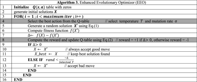
The overall steps of the proposed EEO model are illustrated in Algorithm 3. Basically, EEO consists of two main stages which are Q-learning stage, and SA stage. The details of these stages are explained as follows.
Stage I:
-
Q-learning execution Q-learning algorithm is embedded into SA algorithm as shown in lines 4, and 8 of Algorithm 3. As can be seen that In line 4 of EEO algorithm is responsible about fetching the best action from Q-table. The general structure of the implemented Q-table is given in Fig. 5. As can be seen it consists of nine states which are S1 (T is high, and σ is high), S2 (T is high, and σ is medium), S3 (T is high, and σ is low), S4 (T is medium, and σ is high), S5 (T is medium, and σ is medium), S6 (T is medium, and σ is low), S7 (T is low, and σ is low), S8 (T is low, and σ is medium), S9 (T is low, and σ is low).
Fig. 5 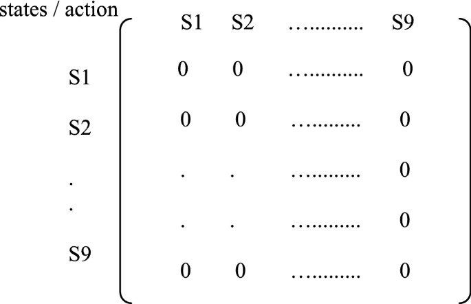
The initial Q-table structure
-
According to the selected action, SA will generate a new solution based on mutation rate \(\upsigma\) (lines 5 and 6 in Algorithm 3). It is worth mentioned that, the reward value is +1 if the fitness value of search vector \(X\) was improved, otherwise is set to − 1. Figure 6 shows all implemented nine states with different actions that makes the implemented algorithm moves from state to another or even remain in the same state.
Fig. 6 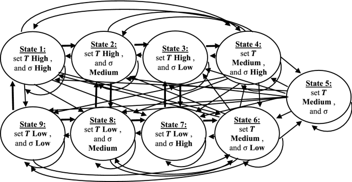
The implemented states of the proposed algorithm
-
It should be noted that the execution of EEO algorithm in [18], resulted in a negligible extra time cost from embedding of Q-learning algorithm. In addition, Algorithm 3 shows that Q-learning algorithm has been efficiently embedded into lines 4, and 8. Also, it required two simple computational operations which are fetch best action and update Q-table.


Stage II:
-
SA execution According to the selected value of temperature rate \(T\) make search vector \(X\) to make a bad movement with probability of \(rand < \frac{ - \Delta }{Selected\_T}\). It is worth mentioned that SA now becomes dynamic in its execution and it can switch from exploration mode to exploitation mode many times during the search progress by changing the value of \(T\). The reaming steps of SA algorithm are identical to Algorithm 1 except the temperature rate which changing according to the generated action by Q-learning algorithm.

3 Face sketch recognition
The proposed architecture of face sketch recognition model is illustrated in Fig. 8 and it consist of three steps i.e. sketch facial components (i.e. eyes, nose, and mouth region) localization using EEO, histogram of gradient (HOG) [24] feature extraction, and components matching. The cosine similarity measure is used for matching and it defined as:
where vectors A and \(B\) represent HOG feature vector. It should be noted that during components localization step vector \(A\) represent currently localized components and vector \(B\) represent the average HOG from training sketched components. However, in final matching stage (step 3), vector \(A\) represents the HOG of the final outcomes of localization step and vector \(B\) is HOG of database photos components during testing stage.
The proposed localization encoding scheme is shown in Fig. 7 and it contains four variables which are \(X,Y,W,\;{\text{and}}\;H\). Variables \(X\) and \(Y\) represent the location of the right eye landmark location. Variables \(W\) and \(H\) represent the width and height of the red coloured box shown in Fig. 8. Based on the localized box (in red colour), eyes, nose, and mouth sketch facial components are generated.

Sketch facial components and the proposed encoding scheme

Face sketch recognition model
3.1 HOG feature extractor
There are many features extraction techniques were employed in the literature for face and face sketch recognition such as HOG [25], LBP [3, 26], and Wavelet [27]. Among them HOG showed superior performances as indicated in our previous research [15, 25]. As such, this work adopts HOG [24] to encode face sketched components (i.e. eyes, nose, and mouth). As can be seen in Fig. 9 that HOG is computed by scanning the input component. A total of three parameters are associated with HOG namely cell, block, and block overlap ratio. The standard settings of HOG are used here [24]. After the scanning process, a gradient vector is generated by binning the magnitude of the gradients at different directions as can be seen in Fig. 9.

The steps of HOG feature extractor
4 Experimental results
This section evaluates the performance of the proposed face sketch recognition approach on various benchmark images. In particular, a total of three face sketch databases are employed which are LFW, AR, and CUHK. In order to compare the outcomes of the proposed optimizer, the most popular optimization algorithms where adopted in this study which are SA [28], PSO [29], MVO [30], and Harmony [31]. The maximum fitness evaluations i.e. FEs was set to \(10^{5}\) for all studied optimization algorithms.
4.1 LFW database
LFW [32] consists of 99 sketch-photo pairs and a number of sample images are shown in Fig. 10. In this experiment a total of 19 randomly chosen sketch-photo pairs have been used for training and the remaining set 80 pairs were used for testing. Each optimization algorithm was executed for 30 times using the same training and testing set. The mean recognition rate for rank-1 was computed and reported in Table 1. As can be observed, the proposed EEO algorithm is able to yield 48.75% rank-1 recognition accuracy which is about 18.75% better than MVO algorithm. It should be noted that the performances of all optimization was low on this database problem. The poor recognition performance is due to many reason such as poor illumination condition of face photos, and pose variations with complicated background that exists in LFW database. Two incorrectly recognized cases are shown in Fig. 11.

Sample images from LFW database

Incorrectly recognized cases
4.2 AR database
In this section the proposed EEO algorithm was evaluated on AR [33] sketches. AR database comprises a total of 123 sketch-photo pairs and it is one of the most popular sketch database that has been used in the literature [34, 35]. In this experiment, a randomly chosen 100 sketches have been used for testing and the remaining 23 sketches were used for training as in [34]. Each optimization algorithm was executed for 30 times and the mean rank-1 value of the achieved results are summarized in Table 2. As can be observed, the reported mean recognition rate of rank-1 from EEO algorithm outperform others algorithms. The worst recognition rate was observed with Harmony and MVO. However, PSO and SA have shown good performances due to their ability to exploit the search space more efficiently as compared with other algorithms [16].
Further analysis was conducted by measuring the percentage of overlap between the localized sketch facial components (i.e. eyes, nose, and mouth) as compared with the ground truth. The mean, minimum, and maximum achieved results from all optimizer for 30 runs was computed and shown in Fig. 12. As indicated, EEO was able to report the best results among other algorithms. It can be seen that the box plot of EEO was more compact. On the other hand, the intervals between the maximum and minimum value of box plot for other algorithms was much larger than EEO. This implies that EEO model was stable in locating sketch facial components during multiple runs.

The percentage of overlap measure for different facial sketch component a eyes, b mouth and c nose
To evaluate the outcomes of EEO statistically, the bootstrap method [36] with 95% confidence intervals of EEO results were computed. Table 3 reports the results and it should be noted that the lower bound of the confidence interval represents the worst performance achieved by EEO. As can be observed in Table 3, the statistical outcomes of the proposed model significantly outperform other methods. In other words, the reported mean values by other methods were much lower than the confidence interval reported by EEO. This is due to the advantage of component-based technique as compared with holistic-based methods [10]. Moreover, EEO was efficient in locating sketch facial components.
4.3 CUHK database
In this analysis, the database of CUHK [4] is used to evaluate EEO performances. CUHK consists of 188 sketch-photo pairs and a number of images are shown in Fig. 13. In this experiment, a randomly chosen 138 sketches were used for testing and the remaining 50 sketches were used for training as in [34]. This experiment was executed for 30 times and the mean Rank-1 recognition rate from each optimization algorithm is given in Table 4. The reported results confirm the applicability of EEO algorithm where it can outperform others studied optimization algorithms i.e. SA, PSO, MVO, and Harmony. As explained earlier that EEO has the advantage of embedded Q-learning algorithm. As mentioned earlier that EEO is dynamic in its execution where it switches adaptively from exploration to exploitation mode according to search performances. More importantly, the statistical outcomes (95% confidence intervals) confirm the performances statically.

Sample images from CUHK database
Further analysis was conducted by comparing the outcomes of EEO algorithm with other results published in the literature. In particular, the outcomes from Stringface [34], DCP [35], PCA [37], and LMCFL [38] where reported in Table 5. The reported results indicate that EEO is able to outperform other models statically with 95% confidence level.
5 Conclusions
A component-based face sketch recognition technique is introduced in this work. An efficient EEO model is used to locate the components. The proposed approach is evaluated on three face sketch benchmark datasets namely AR, LFW, and CUHK. The outcomes indicate superior performances of EEO to locate the components as compared SA and other optimization algorithms including PSO, Harmony, and MVO. From the statistical point of view, the archived results by EEO significantly outperform other results published in the literature on AR, and CUHK benchmark images. Further studied could be investigated by applying EEO on face and others image-based pattern recognition problems.
References
Xiaoou T, Xiaogang W (2004) Face sketch recognition. IEEE Trans Circuits Syst Video Technol 14(1):50–57
Roy H, Bhattacharjee D (2016) Face sketch-photo matching using the local gradient fuzzy pattern. IEEE Intell Syst 31(3):30–39
Klare BF, Zhifeng L, Jain AK (2011) Matching forensic sketches to mug shot photos. IEEE Trans Pattern Anal Mach Intell 33(3):639–646
Wang X, Tang X (2009) Face photo-sketch synthesis and recognition. IEEE Trans Pattern Anal Mach Intell 31(11):1955–1967
Wang N et al (2017) Unified framework for face sketch synthesis. Sig Process 130:1–11
Hu W, Hu H (2018) Fine tuning dual streams deep network with multi-scale pyramid decision for heterogeneous face recognition. Neural Process Let. https://doi.org/10.1007/s11063-018-9942-1
Jiao L et al (2018) A modified convolutional neural network for face sketch synthesis. Pattern Recogn 76:125–136
Lee W-Y, Park S-M, Sim K-B (2018) Optimal hyperparameter tuning of convolutional neural networks based on the parameter-setting-free harmony search algorithm. Optik 172:359–367
Jiang J et al (2019) Graph-regularized locality-constrained joint dictionary and residual learning for face sketch synthesis. IEEE Trans Image Process 28(2):628–641
Liu D et al (2018) Composite components-based face sketch recognition. Neurocomputing 302:46–54
Hu H et al (2013) Matching composite sketches to face photos: a component-based approach. IEEE Trans Inf Forensics Secur 8(1):191–204
Mittal P et al (2017) Composite sketch recognition using saliency and attribute feedback. Inf Fusion 33:86–99
Kute RS, Vyas V, Anuse A (2019) Component-based face recognition under transfer learning for forensic applications. Inf Sci 476:176–191
Agrawal S, Singh RK, Singh UP, Jain S (2019) Biogeography particle swarm optimization based counter propagation network for sketch based face recognition. Multimed Tools Appl 78(8):9801–9825
Samma H, Suandi SA, Mohamad-Saleh J (2018) Face sketch recognition using a hybrid optimization model. Neural Comput Appl. https://doi.org/10.1007/s00521-018-3475-4
Samma H, Lim CP, Saleh JM (2016) A new reinforcement learning-based memetic particle swarm optimizer. Appl Soft Comput 43:276–297
Samma H, Lim CP, Ngah UK (2013) A hybrid PSO-FSVM model and its application to imbalanced classification of mammograms. In: Asian conference on intelligent information and database systems. Springer, Berlin, pp 275–284
Samma H et al (2019) Q-learning-based simulated annealing algorithm for constrained engineering design problems. Neural Comput Appl 1–15
Van Laarhoven PJ, Aarts EH (1987) Simulated annealing. In: Simulated annealing: theory and applications. Springer, pp 7–15
Watkins CCH, Dayan P (1992) Q-learning. Mach Learn 8(3–4):279–292
McPartland M, Gallagher M (2011) Reinforcement learning in first person shooter games. IEEE Trans Comput Intell AI Games 3(1):43–56
Sharma R, Spaan MTJ (2012) Bayesian-game-based fuzzy reinforcement learning control for decentralized POMDPs. IEEE Trans Comput Intell AI Games 4(4):309–328
Rakshit P et al (2013) Realization of an adaptive memetic algorithm using differential evolution and q-learning: a case study in multirobot path planning. IEEE Trans Syst Man Cybern Syst 43(4):814–831
Dalal N, Triggs B (2005) Histograms of oriented gradients for human detection. In: Computer vision and pattern recognition. IEEE, San Diego, CA, USA
Samma H, Suandi SA (2017) Application of particle swarm optimization in face sketch recognition. Adv Sci Lett 23(11):11228–11232
Khan SA, Usman M, Riaz N (2015) Face recognition via optimized features fusion. J Intell Fuzzy Syst 28(4):1819–1828
Khan SA et al (2018) Face recognition under varying expressions and illumination using particle swarm optimization. J Comput Sci 28:94–100
Kirkpatrick S, Gelatt CD, Vecchi MP (1983) Optimization by simulated annealing. Science 220(4598):671–680
Kennedy J, Eberhart R (1995) Particle swarm optimization. In: Proceedings of IEEE international conference on neural networks
Mirjalili S, Mirjalili SM, Hatamlou A (2016) Multi-verse optimizer: a nature-inspired algorithm for global optimization. Neural Comput Appl 27(2):495–513
Zhao SZ et al (2011) Dynamic multi-swarm particle swarm optimizer with harmony search. Expert Syst Appl 38(4):3735–3742
Huang GB et al (2007) Labeled faces in the wild: a database for studying face recognition in unconstrained environments. Technical report 07-49, University of Massachusetts, Amherst
Martinez A, Benavente R (2007) The AR face database, 1998. Computer vision center, technical report, 3
Weiping C, Yongsheng G (2013) Face recognition using ensemble string matching. IEEE Trans Image Process 22(12):4798–4808
Gao Y, Qi Y (2005) Robust visual similarity retrieval in single model face databases. Pattern Recogn 38(7):1009–1020
Efron B (1979) Bootstrap methods: another look at the jackknife. Ann Stat 7(1):1–26
Turk M, Pentland A (1991) Eigenfaces for recognition. J Cogn Neurosci 3(1):71–86
Jin Y, Lu J, Ruan Q (2015) Large margin coupled feature learning for cross-modal face recognition. In: 2015 international conference on biometrics (ICB). IEEE
Acknowledgements
This paper was fully supported by Universiti Sains Malaysia (USM) Short Term Research Grant (Grant No. 304/PELECT/6315293).
Author information
Authors and Affiliations
Corresponding author
Ethics declarations
Conflict of interest
The authors declare that they have no conflict of interest.
Additional information
Publisher's Note
Springer Nature remains neutral with regard to jurisdictional claims in published maps and institutional affiliations.
Rights and permissions
About this article

Cite this article
Samma, H., Suandi, S.A. & Mohamad-Saleh, J. Component-based face sketch recognition using an enhanced evolutionary optimizer. SN Appl. Sci. 1, 939 (2019). https://doi.org/10.1007/s42452-019-0981-7
Received:
Accepted:
Published:
DOI: https://doi.org/10.1007/s42452-019-0981-7