Reconstructing toric quiver flag varieties from a tilting bundle

Abstract

We prove that every toric quiver flag variety Y is isomorphic to a fine moduli space of cyclic modules over the algebra $\mathrm{End}(T)$ for some tilting bundle T on Y. This generalises the well-known fact that can be recovered from the endomorphism algebra of .

1 Introduction

Nakajima [8, Section 3] introduced certain framed moduli spaces associated to a quiver, and the first author showed that these ‘quiver flag varieties’ admit a tilting bundle [3], generalising the construction of Beilinson [1] and Kapranov [6]. Here we extend this link further in the toric case by showing that every toric quiver flag variety can be reconstructed as a fine moduli space of cyclic modules over the endomorphism algebra of the tilting bundle.

Before stating the main result we recall the construction and basic geometric properties of quiver flag varieties, also known as ‘framed quiver moduli’; references for this material include Nakajima [8, Section 3], Reineke [9] and Craw [3]. Let $\Bbbk$ be an algebraically closed field of characteristic zero and let Q be a finite, connected, acyclic quiver with a unique source. Write for the vertex set, where 0 is the source, and $Q_1$ for the arrow set, where for each $a\in Q_1$ we write $\mathrm{h}(a)$ and $\mathrm{t}(a)$ for the head and tail of a respectively. Fix a dimension vector satisfying . The group acts by conjugation on the space of representations of Q of dimension vector $\underline{r}$, and we define the quiver flag variety associated to the pair $(Q,\underline{r})$ to be the GIT quotient

for the special choice of linearisation . This GIT quotient is non-empty if and only if the inequality

(1)

holds for each $i>0$, in which case Y is a smooth Mori Dream Space of dimension . In fact, Y can be obtained from a tower of Grassmann-bundles

(2)

where at each stage, $Y_i$ is isomorphic to the Grassmannian of rank $r_i$ quotients of a fixed locally-free sheaf of rank $s_i$ on $Y_{i-1}$; see [3, Theorem 3.3]. Hereafter we assume that the inequality (1) is strict for each $i>0$ to avoid degeneracy in the tower.

Quiver flag varieties naturally carry a collection of vector bundles $\mathscr {W}_1,\dots , \mathscr {W}_\ell$ that determine many of their algebraic invariants. Indeed, for $i>0$, the Grassmann-bundle $Y_i$ over $Y_{i-1}$ carries a tautological quotient bundle $\mathscr {V}_i$ of rank $r_i$, and we write for the globally-generated bundle of rank $r_i$ on Y obtained as the pullback under the morphism $\pi _i:Y\rightarrow Y_i$ in the tower. It follows from the construction that the invertible sheaves provide an integral basis for the Picard group of Y. More generally, the results of Beilinson [1] and Kapranov [6] extend to all quiver flag varieties as follows. Let denote the set of Young diagrams with no more than k columns and l rows. Recall that for any vector bundle $\mathscr {W}$ of rank r and for , we obtain a vector bundle whose fibre over each point is the irreducible -module of highest weight $\lambda$.

Theorem 1.1

([3]) The vector bundle on Y given by

(3)

is a tilting bundle. In particular, the bounded derived category of coherent sheaves on Y is equivalent to the bounded derived category of finite-dimensional modules over .

This result answered affirmatively the question of Nakajima [8, Problem 3.10].

We now describe our main result. Work of Bergman and Proudfoot [2, Theorem 2.4] compares any smooth projective variety admitting a tilting bundle to a fine moduli space of modules over the endomorphism algebra. To define the relevant moduli space for the tilting bundle E from (3), list the indecomposable summands as $E_0, E_1,\dots , E_n$ with , and consider the dimension vector satisfying for all $0\leqslant j\leqslant n$. For a special choice of ‘0-generated’ stability condition $\theta$ (see Sect. 2), we consider the fine moduli space $\mathscr {M}(A,\varvec{\mathrm v},\theta )$ of isomorphism classes of $\theta$-stable A-modules of dimension vector $\varvec{\mathrm v}$ that was constructed by King [7] using GIT. Since each bundle is globally-generated, an observation of Craw et al. [4, Theorem 1.1] induces a universal morphism

$$\begin{aligned} f_E:Y\rightarrow \mathscr {M}(A,\varvec{\mathrm v},\theta ), \end{aligned}$$

(4)

and in our case this is a closed immersion. In fact, [2, Theorem 2.4] implies that $f_E$ identifies Y with a connected component of $\mathscr {M}(A,\varvec{\mathrm v},\theta )$, because Y is smooth, E is a tilting bundle, and our stability condition $\theta$ is ‘great’.

Our main result concerns the special case when for all $1\leqslant i\leqslant \ell$, in which case G is an algebraic torus and therefore Y is a toric variety; we call Y a toric quiver flag variety. The toric fan $\Sigma$ can be described directly in this case (see [5, p. 1517]), and Y is a tower of projective space bundles via (2). We can say the following:

Theorem 1.2

Let Y be a toric quiver flag variety. The morphism from (4) is an isomorphism.

As a result, toric quiver flag varieties provide a new class of examples where the programme of Bergman and Proudfoot [2] can be carried out in full, enabling one to reconstruct the variety from the tilting bundle. The special case where Y is isomorphic to projective space recovers the well-known result that can be reconstructed from the tilting bundle of Beilinson [1]. Theorem 1.2 therefore provides further evidence that toric quiver flag varieties provide good multigraded analogues of projective space.

2 The reduction step

Our assumption gives for $1\leqslant i\leqslant \ell$, so the tilting bundle from (3) is simply the direct sum of line bundles

(5)

on Y. Set , and list the indecomposable summands from (5) as $E_0, \dots , E_{n}$ with . Consider the endomorphism algebra and the dimension vector .

The moduli space that features in Theorem 1.2 is an example of those constructed originally by King [7]. To introduce our choice of stability condition, first set . An A-module of dimension vector $\varvec{\mathrm v}$ is $\theta ^\prime$-stable iff M is generated as an A-module by any nonzero element of $M_0$; any such stability condition is called 0-generated. Since $\varvec{\mathrm v}$ is primitive and since every $\theta ^\prime$-semistable A-module of dimension vector $\varvec{\mathrm v}$ is $\theta ^\prime$-stable (see, for example, [5, Proof of Proposition 3.8]), King [7, Proposition 5.3] constructs the fine moduli space $\mathscr {M}(A,\varvec{\mathrm v},\theta ^\prime )$ of isomorphism classes of $\theta ^\prime$-stable A-modules of dimension vector $\varvec{\mathrm v}$ as a GIT quotient. In particular, $\mathscr {M}(A,\varvec{\mathrm v},\theta ^\prime )$ comes with an ample bundle $\mathscr {O}(1)$. Let $k\geqslant 1$ denote the smallest positive integer such that is very ample. Then is also a 0-generated stability condition, and we consider the fine moduli space $\mathscr {M}(A,\varvec{\mathrm v}, \theta )$ of $\theta$-stable A-modules of dimension vector $\varvec{\mathrm v}$; this moduli space is the ‘multigraded linear series’ of E in the sense of [4, Definition 2.5].

Since each indecomposable summand of E from (5) is globally-generated, we deduce from [4, Theorem 2.6] that the universal property of $\mathscr {M}(A,\varvec{\mathrm v}, \theta )$ gives a morphism

$$\begin{aligned} f_E:Y\rightarrow \mathscr {M}(A,\varvec{\mathrm v},\theta ) \end{aligned}$$

and, moreover, $f_E$ is a closed immersion because the line bundle is very ample. This puts us in the situation studied by Craw and Smith [5], where it is possible to give an explicit GIT quotient description for both the moduli space $\mathscr {M}(A,\varvec{\mathrm v},\theta )$ and the image of the universal morphism $f_E$. Theorem 1.2 will follow once we prove that these two GIT quotients coincide.

To describe $\mathscr {M}(A,\varvec{\mathrm v},\theta )$ as a GIT quotient, we first present the algebra $A=\mathrm{End}_{\mathscr {O}_Y}(E)$ using the bound quiver of sections $(Q^\prime \!,R)$ as follows. The quiver $Q^\prime$ has vertex set and an arrow from vertex i to j for each irreducible, torus-invariant section of , i.e., the corresponding homomorphism from $E_i$ to does not factor through some $E_k$ with $k \ne i, j$. To each arrow $a\in Q^\prime _1$ we associate the corresponding torus-invariant ‘labeling divisor’ $\mathrm{div}(a)\in \mathbb {N}^{\Sigma (1)}$, where $\Sigma (1)$ denotes the set of rays of the fan of Y. The two-sided ideal

in $\Bbbk Q^\prime$ satisfies (see [5, Proposition 3.3]). Denote the coordinate ring of $\mathbb {A}^{Q^\prime _1}_\Bbbk$ by , where a ranges over $Q^\prime _1$. The ideal R in the noncommutative ring $\Bbbk Q^\prime$ determines an ideal in given by

(6)

where the support of a path $\mathrm{supp}(p)$ is simply the set of arrows that make up the path. This ideal is homogeneous with respect to the action of by conjugation. It now follows directly from the definition of King [7] that

(7)

where denotes the $k\theta$-graded piece. In fact, [5, Proposition 3.8] implies that $\mathscr {M}(A,\varvec{\mathrm v},\theta )$ is the geometric quotient of by the action of T, where

(8)

is the irrelevant ideal in that cuts out the $\theta$-unstable locus in $\mathbb {A}_\Bbbk ^{\!Q^\prime _1}$.

Our task is to compare (7) with the GIT quotient description of the image of $f_E$. For this, define a map by setting $\pi (\chi _a)=(\chi _{\mathrm{h}(a)}-\chi _{\mathrm{t}(a)},\mathrm{div}(a))$, where $\chi _a$ for $a\in Q^\prime _1$ and $\chi _i$ for $i\in Q^\prime _0$ denote the characteristic functions. The T-homogeneous ideal

(9)

contains $I_R$ from (6), and [5, Proposition 4.3] establishes that the image of the universal morphism $f_E$ is isomorphic to the geometric quotient of by the action of T.

Proposition 2.1

Suppose that the T-orbit of every closed point of contains a closed point of . Then Theorem 1.2 holds.

Proof

The inclusion $\mathbb {V}(I_{Q^\prime })\subseteq \mathbb {V}(I_R)$ always holds, and the assumption ensures that , so the closed immersion $f_E$ is surjective. $\square$

In Sect. 4 we prove that the assumption of Proposition 2.1 holds for every toric quiver flag variety Y. To illustrate the strategy, we recall the following well-known construction of using Beilinson’s tilting bundle.

Example 2.2

For the acyclic quiver Q with vertex set and $n+1$ arrows from 0 to 1, the toric quiver flag variety Y is isomorphic to and the quiver of sections $Q^\prime$ for the tilting bundle is shown in Fig. 1; note that Q is a subquiver of $Q^\prime$. For each $1\leqslant m\leqslant n$ and each ray $\rho \in \Sigma (1)$ in the fan of defining a torus-invariant divisor , let $a_\rho ^m$ denote the arrow with head at m and labeling divisor . Writing for the variable associated to the arrow $a_\rho ^m$, we have

(10)

We claim that a point lies in the same T-orbit as the point $(v_\rho ^m)$ with components for all $1\leqslant m\leqslant n$ and $\rho \in \Sigma (1)$. Clearly , so the claim and Proposition 2.1 show that Theorem 1.2 holds for .

Fig. 1

The tilting quiver of $\mathbb {P}^{n}$

To prove the claim, note that since $(w_\rho ^m)\not \in \mathbb {V}(B_{Q^\prime })$, the T-action allows us to assume that for all $1\leqslant m\leqslant n$ there exists $\rho (m)\in \Sigma (1)$ such that . Then , and (10) implies that for all $\rho \in \Sigma (1)$. The case $\rho =\rho (2)$ gives , so

$$\begin{aligned} w^2_\rho = v^1_\rho (w^1_{\rho (2)})^{-1}= w^1_\rho (w^1_{\rho (2)})^{-1} \quad \text {for all}\;\;\rho \in \Sigma (1). \end{aligned}$$

Let the one-dimensional subgroup scale by at vertex 2 to obtain a point in the same T-orbit as $(w_\rho ^m)$ whose components agree with those of $(v_\rho ^m)$ for $m=1,2$. Repeating at each successive vertex shows that $(v_\rho ^m)$ and $(w_\rho ^m)$ lie in the same T-orbit as claimed.

3 The tilting quiver

Before establishing that the assumption of Proposition 2.1 holds for every toric quiver flag variety, we describe the tilting quiver $Q^\prime$ in detail (see Example 3.3).

For the vertex set $Q^\prime _0$, recall that the line bundles $\mathscr {W}_1, \dots , \mathscr {W}_\ell$ provide an integral basis for $\mathrm{Pic}(Y)\cong \mathbb {Z}^{\ell }$. Since $Q^\prime _0$ is defined by the summands of the tilting bundle E from (5), it is convenient to realise $Q^\prime _0$ as the set of lattice points of a cuboid in of dimension $\ell$ with side lengths $s_1-1,\dots ,s_{\ell }-1$. We label the vertex for by the corresponding lattice point , giving

We introduce a total order on $Q^\prime _0$: for , , write $k<m$ if for the largest index i satisfying .

For the arrow set $Q^\prime _1$, note first that Q is the quiver of sections of , so the arrows in Q correspond precisely to the torus-invariant prime divisors in Y [5, Remark 3.9]. For $\rho \in \Sigma (1)$ we write for the arrow corresponding to the divisor of zeros of a torus-invariant section of . Each $a_\rho$ may be regarded as an arrow in $Q^\prime$, so we may identify Q with a complete subquiver of $Q^\prime$ that we call the base quiver in $Q^\prime$. More generally, translating each $a_\rho$ around the cuboid described in the preceding paragraph (so that the head and tail lie in $Q^\prime _0$) produces arrows in $Q^\prime$ that we denote for $m=\mathrm{h}(a_\rho ^m)$ and . In fact, we have the following:

Lemma 3.1

Every arrow $a\in Q^\prime _1$ is of the form $a=a^m_\rho$, where $m=\mathrm{h}(a)$ and .

Proof

For $a\in Q^\prime _1$, write and , so $\mathrm{div}(a)$ is the divisor of zeros of a section of . In terms of prime divisors, we have

Let $1\leqslant k\leqslant \ell$ be the largest value such that for some $\rho \in \Sigma (1)$ satisfying $k=\mathrm{h}(a_\rho )\in Q_0$. Note that , and moreover, . Since $\mathrm{div}(a)$ is irreducible, translating $a_\rho$ so that the tail is at vertex $m^\prime$ forces the head to lie outside the cuboid, giving or ; similarly, translating $a_\rho$ so that the head is at m forces the tail to lie outside the cuboid, giving or . Since , both and must hold, so . As a result, there must exist $\sigma \in \Sigma (1)$ satisfying for $j=\mathrm{h}(a_{\sigma })$. If we set and repeat the argument above, we deduce that . Continuing in this way, we eventually find $\tau \in \Sigma (1)$ such that with $\mathrm{h}(a_\tau ) = 1$ and $\mathrm{t}(a_\tau )=0$. But then , so we can place a translation of $a_\tau$ with head at m and tail in the cuboid (or tail at $m^\prime$ and head in the cuboid). This shows $\mathrm{div}(a)$ is reducible, a contradiction. $\square$

Remark 3.2

Since Q is the quiver of sections of , the vertices of the base quiver are the vertices , where $e_i$ denotes the $i^{\text {th}}$ standard basis vector for $i>0$, and where .

The next example illustrates how the base quiver sits inside $Q^\prime$.

Example 3.3

The quiver Q shown in Fig. 2, (a) defines the toric quiver flag variety where ; the colours of the arrows indicate the distinct labeling divisors. We have and , so the tilting quiver $Q^\prime$ has 12 vertices shown in Fig. 2, (b) using the ordering described above. Note that the base quiver is the complete subquiver of $Q^\prime$ whose vertices are shown in bold in Fig. 2 (b). The colour of each arrow of $Q^\prime$ is determined by its unique translate arrow from the base quiver.

Fig. 2

Quivers for Y: (a) original quiver Q; (b) tilting quiver $Q^\prime$

4 Proof of Theorem 1.2

In light of Lemma 3.1, each point of $\mathbb {A}^{\!Q^\prime _1}_\Bbbk$ is a tuple $(w_\rho ^m)$ where $w_\rho ^m\in \Bbbk$ for $\rho \in \Sigma (1)$ and for all relevant $m\in Q^\prime _0$. Motivated by Example 2.2, we associate to $(w_\rho ^m)\in \mathbb {A}^{\!Q^\prime _1}_\Bbbk$ an auxiliary point $(v_\rho ^m)\in \mathbb {V}(I_{Q^\prime })\subseteq \mathbb {A}^{\!Q^\prime _1}_\Bbbk$ whose components satisfy

(11)

where for $\rho \in \Sigma (1)$ we write for the component of the point $(w_\rho ^m)$ corresponding to the unique arrow $a_\rho$ in the base quiver satisfying .

Lemma 4.1

If $(w_\rho ^m)\not \in \mathbb {V}(B_{Q^\prime })$, then $(v_\rho ^m)\not \in \mathbb {V}(B_{Q^\prime })$.

Proof

Fix and let $1\leqslant j\leqslant \ell$ be minimal such that . Then for all $\rho$ satisfying $\mathrm{h}(a_\rho )=j\in Q_0$, the arrow $a_\rho ^m$ obtained by translating $a_\rho$ until the head lies at m is an arrow of $Q^\prime$. At least one of the values is nonzero by assumption, and hence for this value of $\rho$ we have as required. $\square$

We now establish notation for the proof of Theorem 1.2. For any , let denote the bound quiver of sections of the line bundles on Y with . Explicitly, is the complete subquiver of $Q^\prime$ with vertex set , and the ideal of relations satisfies

As in Sect. 2, the coordinate ring of the affine space contains ideals and defined as in Eqs. (6), (8) and (9) respectively, each of which is homogeneous with respect to the action of by conjugation. The projection onto the coordinates indexed by arrows $a_\rho ^m$ satisfying $m\leqslant k$, denoted

(12)

is equivariant with respect to the actions of T and . Notice that , and .

Proof of Theorem 1.2

Fix a point and the corresponding point whose components are defined in equation (11). Since $w\not \in \mathbb {V}(B_{Q^\prime })$, the action of T enables us to assume that for all $m\in Q^\prime _0$ there exists $\rho (m)\in \Sigma (1)$ such that . In particular, $v_{\rho (m)}^m=1$ for all relevant $m\in Q^\prime _0$. Now, for , the morphism $\pi _k$ from (12) sends the points w and v to

respectively. We claim that $\pi _k(v)$ lies in the -orbit of $\pi _k(w)$. Given the claim, the special case shows that the point v lies in the T-orbit of the point w, so Theorem 1.2 follows immediately from Proposition 2.1.

We prove the claim by induction on the vertex using the total order on $Q^\prime _0$ from Sect. 3. The case $k=e_0$ is immediate, and for the claim follows from Example 2.2; hereafter we assume that $\ell \geqslant 2$. Suppose the claim holds for all $m<k$, so we may assume that for all $m<k$. It is enough to show for all $\rho \in \Sigma (1)$, that and

(13)

because then we may let the one-dimensional subgroup scale by at vertex k. Before establishing the claim (13), we introduce some notation that we use in the proof.

Notation 4.2

• (a) Recall from Sect. 3 that vertices of the tilting quiver $Q^\prime$ are elements in the lattice $\mathbb {Z}^\ell$, so for $1\leqslant i\leqslant \ell$. Note also (see Remark 3.2) that the standard basis vectors $e_1,\dots , e_\ell$ of $\mathbb {Z}^\ell$ denote certain vertices of $Q^\prime$. This notation is standard and we hope that no confusion arises in what follows.

• (b) It is convenient to distinguish certain elements of $Q_0$ and $\mathbb {Z}^\ell$.

  • First we distinguish certain elements of the vertex set of the original quiver. For the ray appearing in (13), define $0\leqslant \alpha <\beta \leqslant \ell$ by

    

    where is the arrow in the original quiver Q satisfying . Also, let $1\leqslant \delta \leqslant \ell$ be minimal such that the induction vertex satisfies , and define $0\leqslant \gamma <\delta$ by setting

    

    Minimality of $\delta$ implies that either $\gamma =0$ or and, moreover, that $\delta \leqslant \beta$.

  • Next we introduce certain elements of $\mathbb {Z}^\ell$. For any ray $\rho \in \Sigma (1)$, define

    

    where $a_\rho$ is the arrow in the original quiver satisfying (recall that ). In particular, by the previous bullet point we have

    $$\begin{aligned} \underline{d}(\rho (k))=e_\beta -e_\alpha \quad \text {and}\quad \underline{d}(\rho (e_\delta ))=e_\delta -e_\gamma . \end{aligned}$$

We now return to the proof of the claim (13), treating the cases $\delta <\beta$ and $\delta =\beta$ separately.

Fig. 3

Paths of length 2 in Q

Case 1: Suppose first that $\delta <\beta$. In this case we proceed in three steps:

Step 1: Show that equation (13) holds for $\rho =\rho (e_\delta )$ when $\gamma =\alpha =0$ or $\gamma \ne \alpha$. We use generators of the ideal corresponding to pairs of paths in with head at k. Consider paths of length two as in Fig. 3, where for now we substitute and $\rho (e_\delta )$ in place of $\rho _1$ and $\rho _2$. In this case, we claim that each vertex in Fig. 3 lies in the quiver . Indeed, , so its head k and tail $k-e_\beta +e_\alpha$ lie in ; this implies and either $\alpha =0$ or . Also, and either $\gamma =0$ or , so $k-\underline{d}(\rho (e_\delta ))$ is equal to $k-e_\delta +e_\gamma$, which lies in the quiver . For the fourth vertex in Fig. 3, either:

• (i) $\gamma =\alpha =0$, giving , and the inequalities imply that the fourth vertex lies in as claimed; or

• (ii) $\gamma \ne \alpha$, and since $\gamma<\delta <\beta$, the fourth vertex $k-e_\beta +e_\alpha -e_\delta +e_\gamma$ lies in because , either $\alpha =0$ or $k_\alpha < s_\alpha -1$ and either $\gamma =0$ or .

Figure 3 therefore determines a binomial in which implies that

Our induction assumption gives for all $m<k$, and since , we have . In particular, and

which establishes equation (13) for $\rho =\rho (e_\delta )$ when $\gamma =\alpha =0$ or $\gamma \ne \alpha$.

Step 2: Show that equation (13) holds for $\rho =\rho (e_\delta )$ when $\gamma =\alpha \ne 0$. Since , the method from Step 1 applies verbatim unless . In this case, define $0\leqslant \varepsilon < \gamma$ by

giving $\underline{d}(\rho (e_\gamma ))=e_\gamma -e_\varepsilon$. Consider paths of length three as in Fig. 4, where for now we substitute and $\rho (e_\gamma )$ in place of $\rho _1,\rho _2$ and $\rho _3$. Again, we claim that each vertex in Fig. 4 lies in the quiver ; the proof is similar to that from Step 1 (here, minimality of $\delta$ implies $\varepsilon =0$ or , and we use the inequalities $\varepsilon<\gamma<\delta <\beta$). Thus we obtain a binomial in which, applying the inductive assumption for all $m<k$, gives

Since , we have and which implies that equation (13) holds for $\rho =\rho (e_\delta )$.

Fig. 4

Certain paths of length 3 in Q

Step 3: Show that equation (13) holds for all $\rho \in \Sigma (1)$. Consider any arrow $a_\rho ^k$ in $Q^\prime$ with head at k. The vertices

satisfy $\underline{d}(\rho )=e_\mu -e_\lambda$ with $0\leqslant \lambda <\mu \leqslant \ell$. We proceed using the approach from Steps 1–2:

• (i) If $\mu \ne \beta$, then we substitute $\rho$ and in place of $\rho _1$ and $\rho _2$ in Fig. 3 as in Step 1, unless $\lambda =\alpha \ne 0$ and $s_\alpha =2$ in which case we substitute $\rho (e_\alpha )$ in place of $\rho _3$ in Fig. 4 as in Step 2. In either case, we obtain an equation relating components of $w_k$ which, after applying the inductive hypothesis if necessary, becomes

  

  Steps 1 and 2 established , and , so equation (13) holds.

• (ii) Otherwise, $\mu =\beta$. Substitute $\rho (e_\delta )$ and $\rho$ in place of $\rho _1$ and $\rho _2$ in Fig. 3 as in Step 1, unless $\lambda =\gamma \ne 0$ and in which case we substitute $\rho (e_\gamma )$ in place of $\rho _3$ in Fig. 4 as in Step 2. As in part $(\mathrm {i})$ above, we obtain an equation which simplifies to

  

  Steps 1 and 2 established , so equation (13) follows.

This completes the proof of equation (13) in Case 1.

Case 2: Suppose instead that $\delta =\beta$. If then the proof is identical to Case 1. If on the other hand , then the vertex that plays a key role in Case 1 does not lie in . In the special case that $k=e_\delta$, making k a vertex of the base quiver, then we have for all relevant $\rho \in \Sigma (1)$ and there is nothing to prove. If $k\ne e_\delta$, we introduce another useful vertex of the original quiver: let $\xi$ be minimal such that $\delta <\xi \leqslant \ell$ and , and define $0\leqslant \eta <\xi$ by setting

giving $\underline{d}(\rho (e_\xi ))=e_\xi -e_\eta$. We treat the cases $\eta \ne \delta$ and $\eta =\delta$ separately.

Subcase 2A: If , then either $\eta =0$ or , so $k-\underline{d}(\rho (e_\xi )) = k-e_\xi +e_\eta$ is a vertex of . We may now proceed just as in Case 1 except that $\rho (e_\xi )$ replaces $\rho (e_\delta )$ throughout (so $\xi$ and $\eta$ replace $\delta$ and $\gamma$ respectively).

Subcase 2B: Suppose instead that . We have already reduced to the case . If then once again, $k-\underline{d}(\rho (e_\xi )) = k-e_\xi +e_\delta$ is a vertex of and we proceed as in Case 1 with $\rho (e_\xi )$ replacing $\rho (e_\delta )$ throughout. If , then we proceed as follows:

Step 1: Show that . If $\gamma \ne \alpha$ or $\gamma =\alpha =0$, then we use Fig. 4 with , and to obtain the equation

which gives . Otherwise, $\gamma =\alpha \ne 0$, giving . It may be that , in which case and hence as required. If , then consider the pair of paths of length four as in Fig. 5, where we substitute and $\rho (e_\gamma )$ in place of $\rho _1,\dots ,\rho _4$ (in fact, both paths pass through the same set of vertices in this case).

We obtain the equation

which gives and completes Step 1.

Step 2: Show that equation (13) holds for all $\rho \in \Sigma (1)$. For any , the vertices

satisfy $\underline{d}(\rho )=e_\mu -e_\lambda$ with $0\leqslant \lambda <\mu \leqslant \ell$.

• (i) If $\mu >\delta$, use Fig. 3 with and , unless $\lambda =\alpha \ne 0$ and in which case use Fig. 4 with the addition of . Either way, we obtain the equation which, since by Step 1, gives (13).

• (ii) If $\mu =\delta$, use Fig. 4 with , and unless $\lambda =\alpha \ne 0$ and in which case use Fig. 5 with the addition of . Either way, we obtain which, since by Step 1, gives (13).

This concludes the proof in Case 2, and completes the proof of Theorem 1.2. $\square$

Remark 4.3

Our approach relies on the explicit description of the image of the morphism $f_E$ in Theorem 1.2 as the GIT quotient $\mathbb {V}(I_{Q^\prime })/\!\!/\!_\theta T$, see [5, Theorem 1.1]. We do not at present have a similar description in the non-toric setting.

Example 4.4

We conclude with an example to illustrate the proof of Theorem 1.2. Let Q and $Q^\prime$ be the quivers in Fig. 2, so $\ell =3$. Suppose $k=(0,1,1)\in Q^\prime _0$, so $\delta =2$. The three arrows with head at k have tails at (1, 1, 0) (light blue), (0, 0, 1) (red) and (1, 0, 1) (blue), and we label the corresponding rays $\rho _1, \rho _2$ and $\rho _3$ respectively. We now illustrate in two different situations why and why the equation from (13) holds for $\rho =\rho _1, \rho _2, \rho _3$.

Fig. 5

Certain paths of length 4 in Q

• (a) Suppose that . Then $\beta =3$ and $\alpha =1$ (see Fig. 2, (a)), and . Suppose $\rho (e_\delta )=\rho (e_2)=\rho _2$ so that $\gamma =0$ and . This is an example of Case 1 as $\delta <\beta$, and since $\gamma =0$ we require only Step 1. In this case Fig. 3 becomes

  

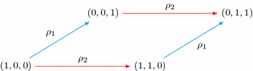
  and the relation gives the equation . Moreover, implies and which establishes (13) for $\rho =\rho _1, \rho _2$. The remaining arrow $a^k_{\rho _3}$ with head at k requires Step 3, and in this case for $\rho =\rho _3$ we have $\mu =2$ and $\lambda =1$. Since and , we require Step 3 (i) to deduce . This implies , establishing (13) for $\rho =\rho _3$.

• (b) Suppose , so $\beta =2$, and . Suppose that $\rho (e_2)=\rho _2$, so $\gamma =0$ and . Since $\delta =\beta$ and , this is an example of Case 2. Since $k\ne e_2$, we compute $\xi =3$. Write $\rho _4$ for the label of the pink arrow with head at (0, 0, 1) and tail at (0, 1, 0), and suppose $\rho (e_3)=\rho _4$. Then $\eta =\mathrm{t}(a_{\rho _4})=2$ and . Since $\eta =\delta$ and , we require Subcase 2B. Following Step 1, since $\gamma =0$ we use Fig. 4 as shown below. This yields the equation which simplifies

  

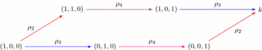
  to $1=w_{\rho _3} w^k_{\rho _2}$, giving as required. Step 2 of Subcase 2B establishes (13) for $\rho =\rho _1,\rho _2,\rho _3$: we already know this for $\rho =\rho _3$ by assumption; the case $\rho =\rho _2$ is provided by Step 1 since ; and the case $\rho =\rho _1$ is a simple application of Step 2 (i), where we apply Fig. 3 to the rectangle with vertices (2, 0, 0), (1, 1, 0), (1, 0, 1), k and arrows labelled $\rho _1$ and $\rho _3$.

References

Beilinson, A.A.: Coherent sheaves on \(\mathbb{P}^{n}\) and problems of linear algebra. Funct. Anal. Appl. 12(3), 214–216 (1978)
Bergman, A., Proudfoot, N.J.: Moduli spaces for Bondal quivers. Pacific J. Math. 237(2), 201–221 (2008)
Craw, A.: Quiver flag varieties and multigraded linear series. Duke Math. J. 156(3), 469–500 (2011)
Craw, A., Ito, Y., Karmazyn, J.: Multigraded linear series and recollement (2017). arXiv:1701.01679 (to appear in Math. Z.)
Craw, A., Smith, G.G.: Projective toric varieties as fine moduli spaces of quiver representations. Amer. J. Math. 130(6), 1509–1534 (2008)
Kapranov, M.M.: On the derived categories of coherent sheaves on some homogeneous spaces. Invent. Math. 92(3), 479–508 (1988)
King, A.D.: Moduli of representations of finite-dimensional algebras. Quart. J. Math. Oxford Ser. 45(180), 515–530 (1994)
Nakajima, H.: Varieties associated with quivers. In: Bautista, R., Martínez-Villa, R., de La Pena, J.A. (eds.) Representation Theory of Algebras and Related Topics. CMS Conference Proceedings, vol. 19, pp. 139–157. American Mathematical Society, Providence (1996)
Reineke, M.: Framed quiver moduli, cohomology, and quantum groups. J. Algebra 320(1), 94–115 (2008)
Acknowledgements
We thank the anonymous referee for a number of helpful comments.
Author information
Authors and Affiliations
Corresponding author
Additional information
The first author was supported in part by EPSRC Grant EP/J019410/1, and the second author is supported by a doctoral studentship from EPSRC.
Rights and permissions
Open Access This article is distributed under the terms of the Creative Commons Attribution 4.0 International License (http://creativecommons.org/licenses/by/4.0/), which permits unrestricted use, distribution, and reproduction in any medium, provided you give appropriate credit to the original author(s) and the source, provide a link to the Creative Commons license, and indicate if changes were made.
About this article
Cite this article
Craw, A., Green, J. Reconstructing toric quiver flag varieties from a tilting bundle. European Journal of Mathematics 4, 185–199 (2018). https://doi.org/10.1007/s40879-017-0194-9
Received:
Revised:
Accepted:
Published:
Issue Date:
DOI: https://doi.org/10.1007/s40879-017-0194-9