
Abstract
Given Hölder continuous functions f and \(\psi \) on a subshift of finite type \(\mathrm{\Sigma }_{A}^{+}\) such that \(\psi \) is not cohomologous to a constant, the classical large deviation principle holds with a rate function \(I_\psi \geqslant 0\) such that \(I_\psi (p) = 0\) iff  , where
  is the equilibrium state of f. In this paper we derive a uniform estimate from below for \(I_\psi \) for p outside an interval containing
  , which depends only on the subshift \(\mathrm{\Sigma }_{A}^{+}\), the function f, the norm \(|\psi |_\infty \), the Hölder constant of \(\psi \) and the integral \(\widetilde{\psi }\). Similar results can be derived in the same way, e.g. for Axiom A diffeomorphisms on basic sets.
1 Introduction
Let \(T:X \rightarrow X\) be a transformation preserving an ergodic probability measure \(\mu \) on a set X. Given an observable \(\psi :X \rightarrow \mathbb {R}\), Birkhoff’s ergodic theorem implies that

for \(\mu \)-almost all \(x\in X\). It follows from general large deviation principles (see [3, 6, 12]) that if X is a mixing basic set for an Axiom A diffeomorphism T, and f and \(\psi \) are Hölder continuous functions on X with equilibrium states
 and \(\mu _\psi \), respectively, and \(\psi \) is not cohomologous to a constant (see the definition below), then there exists a real-analytic rate function
 , where
  , such that

for all  . Here \({\mathscr {M}}_T\) is the set of all T-invariant Borel probability measures on X. Moreover, \(I(p) = 0\) if and only if
  , and the (closed) interval \({\mathscr {I}}_{\psi }\) is non-trivial, since \(\psi \) is not cohomologous to a constant.
Similar large deviation principles apply for any subshift of finite type \(\sigma :\mathrm{\Sigma }_{A}^{+}\rightarrow \mathrm{\Sigma }_{A}^{+}\) on a one-sided shift space

Here A is an  -matrix of 0’s and 1’s (\(s_0\geqslant 2\)). We assume that A is aperiodic, i.e. there exists an integer \(M > 0\) such that
  for all i, j (see, e.g. [7, Chapter 1]). The shift map
\(\sigma \) is defined by \(\sigma (\xi ) = \xi '\), where \(\xi '_i = \xi _{i+1}\) for all \(i \geqslant 0\). We consider \(\mathrm{\Sigma }_{A}^{+}\) with a metric \(d_\theta \) defined for some constant \(\theta \in (0,1)\) by \(d_\theta (\xi ,\eta ) = 0\) if \(\xi = \eta \) and \(d_\theta (\xi ,\eta ) = \theta ^k\) if \(\xi \ne \eta \) and \(k\geqslant 0\) is the maximal integer with \(\xi _i = \eta _i\) for \(0\leqslant i \leqslant k\).
for all i, j (see, e.g. [7, Chapter 1]). The shift map
\(\sigma \) is defined by \(\sigma (\xi ) = \xi '\), where \(\xi '_i = \xi _{i+1}\) for all \(i \geqslant 0\). We consider \(\mathrm{\Sigma }_{A}^{+}\) with a metric \(d_\theta \) defined for some constant \(\theta \in (0,1)\) by \(d_\theta (\xi ,\eta ) = 0\) if \(\xi = \eta \) and \(d_\theta (\xi ,\eta ) = \theta ^k\) if \(\xi \ne \eta \) and \(k\geqslant 0\) is the maximal integer with \(\xi _i = \eta _i\) for \(0\leqslant i \leqslant k\).
For any function \(g:\mathrm{\Sigma }_{A}^{+}\rightarrow \mathbb {R}\) set

Denote by \({\mathscr {F}}_\theta (\mathrm{\Sigma }_{A}^{+})\) the space of all functions g on \(\mathrm{\Sigma }_{A}^{+}\) with \(\Vert g\Vert _\theta < \infty \).
Two functions f, g on \({\mathscr {F}}_\theta (\mathrm{\Sigma }_{A}^{+})\) are called cohomologous if there exists a continuous function h on \(\mathrm{\Sigma }_{A}^{+}\) such that  .
.
The Ruelle transfer operator
 is defined by

Here \(C(\mathrm{\Sigma }_{A}^{+})\) denotes the space of all continuous functions \(g :\mathrm{\Sigma }_{A}^{+}\rightarrow \mathbb {R}\) with respect to the metric \(d_\theta \). Denote by  the topological pressure

of \(\psi \) with respect to the map \(\sigma \), where \({\mathscr {M}}_{\sigma }\) is the set of all \(\sigma \) -invariant probability measures on \(\mathrm{\Sigma }_{A}^{+}\) and \(h_{\sigma }(m)\) is the measure theoretic entropy of m with respect to \(\sigma \) (see [7] or [10]). Given \(\psi \in {\mathscr {F}}_\theta (\mathrm{\Sigma }_{A}^{+})\), there exists a unique \(\sigma \)-invariant probability measure \(\mu _\psi \) on \(\mathrm{\Sigma }_{A}^{+}\) such that

(see, e.g. [7, Theorem 3.5]). The measure \(\mu _\psi \) is called the equilibrium state of \(\psi \).
For brevity throughout we write  for
for  . In what follows we assume that \(\theta \in (0,1)\) is a fixed constant, \(f :\mathrm{\Sigma }_{A}^{+}\rightarrow \mathbb {R}\) is a fixed function in \({\mathscr {F}}_\theta (\mathrm{\Sigma }_{A}^{+})\) and
  .
.
As we mentioned earlier, it follows from the Large Deviation Theorem [3, 6, 12] that if \(\psi \) is not cohomologous to a constant, then there exists a real analytic rate function
 with \(I(p) = 0\) iff
  for which (1) holds. More precisely, we have

It is also known that

and  is a strictly convex function of q (see [7, 10] or [4]).
In his paper we derive an estimate from below for \(I_\psi (p)\) for p outside an interval containing

The estimate depends only on \(|\psi |_\infty ,\widetilde{\psi },|\psi |_\theta \) and some constants determined by the given function f. In what follows we use the notation \(\min \psi = \min _{x\in \mathrm{\Sigma }_{A}^{+}} \psi (x)\),

Since \(\widetilde{\psi }> \min \psi \) (\(\psi \) is not cohomologous to a constant), we have \(\widetilde{\psi }- \min \psi > 0\), so \(B_\psi > 0\) always.
Theorem 1.1
Let \(f, \psi \in {\mathscr {F}}_\theta (\mathrm{\Sigma }_{A}^{+})\) be real-valued functions. Assume that \(\psi \) is not cohomologous to a constant, and let \(0< \delta _0 < B_\psi \). Then for all  we have

where  for some constant \(C >0\) depending only on
  , \(|f|_\theta ,|\psi |_\infty ,\widetilde{\psi }\) and \(\delta _0\).
The motivation to try to obtain estimates of the kind presented in Theorem 1.1 comes from attempts to get some kind of an ‘approximate large deviation principle’ for characteristic functions \(\chi _K\) of arbitrary compact sets K of positive measure. In the special case when the boundary \(\partial K\) of K is ‘relatively regular’ (e.g. \(\mu (\partial K) = 0\)) large deviation results were established by Leplaideur and Saussol in [5], and also by Kachurovskii and Podvigin [2]. The next example presents a first step in the case of an arbitrary compact set K of positive measure.
Example 1.2
Let K be a compact subset of \(\mathrm{\Sigma }_{A}^{+}\) with \(0< \mu (K) < 1\), let \(0 < \delta _0 \leqslant \mu (K)\), and let \(\psi \) be a Hölder continuous function that approximates \(\chi _K\) from above, i.e. \(0 \leqslant \psi \leqslant 1\), \(\psi = 1\) on K and \(\psi = 0\) outside a small neighbourhood V of K. Then \(b = |\psi |_\theta \gg 1\) if V is sufficiently small, so \(q_0\) in Theorem 1.1 has the form \(q_0 = 1/b\). It then follows from Theorem 1.1 (in fact, from Lemma 2.3) that  for
for  .
.
A result similar to Theorem 1.1 can be stated, e.g. for Axiom A diffeomorphisms on basic sets. Recall that if \(F:M \rightarrow M\) is a \(C^1\) Axiom A diffeomorphism on a Riemannian manifold M, a non-empty subset \(\mathrm{\Lambda }\) of M is called a basic set for F if \(\mathrm{\Lambda }\) is a locally maximal compact F-invariant subset of M which is not a single orbit, F is hyperbolic and transitive on \(\mathrm{\Lambda }\), and the periodic points of F in \(\mathrm{\Lambda }\) are dense in \(\mathrm{\Lambda }\) (see, e.g. [1] or [7, Appendix III]). It follows from the existence of Markov partitions that there exists a two-sided subshift of finite type \(\sigma :\mathrm{\Sigma }_A\rightarrow \mathrm{\Sigma }_A\) and a continuous surjective map \(\pi :\mathrm{\Sigma }_A\rightarrow \mathrm{\Lambda }\) such that: (i)  , and (ii) for every Hölder continuous function g on \(\mathrm{\Lambda }\),
  for some \(\theta \in (0,1)\) and \(\pi \) is one-to-one almost everywhere with respect to the equilibrium state of f. Given a Hölder continuous function g on \(\mathrm{\Lambda }\), the rate function \(I_g\) is naturally related to the rate function
  of
of  . On the other hand, f is cohomologous to a function \(f' \in {\mathscr {F}}_{\sqrt{\theta }}(\mathrm{\Sigma }_A)\) which depends on forward coordinates only, so
  . Applying Theorem 1.1 to \(f'\) provides a similar result for f and therefore for g.
For some hyperbolic systems, large deviation principles similar to (1), however with shrinking intervals, have been established recently in [8, 9].
2 Proof of Theorem 1.1
2.1 The Ruelle–Perron–Frobenius Theorem
For convenience of the reader we state here a part of the estimates in [11] that will be used in this section.
Theorem 2.1
(Ruelle–Perron–Frobenius) Let the  -matrix A and \(M > 0\) be as in Sect. 1, let \(f\in {\mathscr {F}}_\theta (\mathrm{\Sigma }_{A}^{+})\) be real-valued, and let
  . Then:
-
(i)
There exist a unique
 , a probability measure
  on \(\mathrm{\Sigma }_{A}^{+}\) and a positive function
 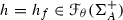 such that
  and
and  . The spectral radius of
  as an operator on \({\mathscr {F}}_\theta (\mathrm{\Sigma }_{A}^{+})\) is \(\lambda \), and its essential spectral radius is \(\theta \lambda \). The eigenfunction h satisfies
Moreover,
for any integer \(n \geqslant 0\).
-
(ii)
The probability measure \(\widehat{\nu } = h\nu \) (this is the so-called equilibrium state of f) is \(\sigma \)-invariant and \(\widehat{\nu } = \nu _{\widehat{f}}\), where
 . Moreover \(L_{\widehat{f}} 1 = 1\).
 -
(iii)
For every \(g\in {\mathscr {F}}_\theta (\mathrm{\Sigma }_{A}^{+})\) and every integer \(n \geqslant 0\) we have
where we can take

and
 , a probability measure
  on
on  such that
  and
and  . The spectral radius of
  as an operator on

 . Moreover


Remark 2.2
The constants that appear in the above estimates are not optimal. The proof of [11, Theorem 2] follows that in [1, Section 1.B] with a more careful analysis of the estimates involved. The main point here is that, apart from their obvious dependence on parameters related to the subshift of finite type \(\sigma :\mathrm{\Sigma }_{A}^{+}\rightarrow \mathrm{\Sigma }_{A}^{+}\), these constants can be taken to depend only on \(| f |_\theta \) and \(| f |_\infty \).
2.2 Reductions
Let \(f \in {\mathscr {F}}_\theta (\mathrm{\Sigma }_{A}^{+})\) be the fixed function from Sect. 1 and let  be as before. It follows from the properties of pressure (see, e.g. [10] or [7]) that
  for every continuous function g and every constant \(c \in \mathbb {R}\). Thus, replacing f by
  , we may assume that
  . Moreover, if g and h are cohomologous continuous functions on \(\mathrm{\Sigma }_{A}^{+}\), then
  and the equilibrium states \(\mu _g\) of g and \(\mu _h\) of h on \(\mathrm{\Sigma }_{A}^{+}\) coincide. Since f is cohomologous to a function \(\phi \in {\mathscr {F}}_\theta (\mathrm{\Sigma }_{A}^{+})\) with \(L_\phi 1 =1\) (see, e.g. [7]), it is enough to prove the main result with f replaced by such a function \(\phi \). Moreover, \(|\phi |_\infty \) and \(|\phi |_\theta \) can be estimated by means of
  and \(|f|_\theta \) [see e.g. Theorem 2.1 (ii)].
So, from now on we will assume that \(L_\phi 1 = 1\). It then follows that  . Let \(\mu = \mu _\phi \) be the equilibrium state of \(\phi \) on \(\mathrm{\Sigma }_{A}^{+}\).
For the proof of Theorem 1.1 we may assume that \(\psi \geqslant 0\). Indeed, assuming the statement of the theorem is true in this case, suppose \(\psi \) takes negative values. Set \(\psi _1 = \psi + c\), where \(c = - \min \psi \). Then \(\psi _1 \geqslant 0\). Moreover,  ,
,  , and for \(p_1 = p+c\) we have

for all \(q \in \mathbb {R}\). Therefore (2) implies

Moreover, if \(0< \delta _0 < B_\psi = B_{\psi _1}\), then  is equivalent to
  . Since \(|\psi _1|_\theta = |\psi |_\theta \) and \(|\psi _1|_\infty \leqslant 2 |\psi |_\infty \), using Theorem 1.1 for \(I_{\psi _1}(p_1)\) and changing appropriately the value of the constant \(q_0\), we get a similar estimate for \(I_\psi (p)\).
2.3 Proof of Theorem 1.1 for \(\psi \geqslant 0\)
From now on we will assume that \(\phi , \psi \in {\mathscr {F}}_\theta (\mathrm{\Sigma }_{A}^{+})\) are fixed real-valued functions such that \(\psi \geqslant 0\), \(\psi \) is not cohomologous to a constant, and
Given any \(q\in \mathbb {R}\), set

In what follows we will assume
for some constant \(q_0 > 0\) which will be chosen below. Then \(|f_q|_\theta \leqslant |\phi |_\theta + 1\) for all q with (5), and also \(|f_q|_\infty \leqslant |\phi |_\infty + |\psi |_\infty \). Thus, setting

we have

Let \(\nu _q\) be the probability measure on \(\mathrm{\Sigma }_{A}^{+}\) with
where \(\lambda _q\) is the maximal eigenvalue of \(L_q = L_{f_q}\), and let \(h_q > 0\) be a corresponding normalised eigenfunction, i.e. \(h_q \in {\mathscr {F}}_\theta (\mathrm{\Sigma }_{A}^{+})\), \(L_qh_q = \lambda _q h_q\) and  . Then \(\mu _q = h_q \nu _q\) is the equilibrium state of \(f_q\), i.e. \(\mu _q = \mu _{\phi + q \psi }\). Clearly \(h_0 = 1\) and \(\mu _0 = \mu \).
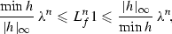
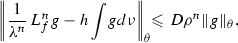
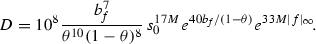
Using the uniform estimates in Theorem 2.1, it follows from (6) that there exist constants \(D \geqslant 1\) and \(\rho \in (0,1)\), depending on \(C_0\) but not on \(q_0\), such that

for all integers \(n \geqslant 0\), all functions \(g \in {\mathscr {F}}_\theta (\mathrm{\Sigma }_{A}^{+})\) and all q with  .
.
Set \(L = L_\phi \). Given \(x \in \mathrm{\Sigma }_{A}^{+}\) and \(m \geqslant 0\), set \(g_m(x) = g(x) + g(\sigma x) + \cdots + g(\sigma ^{m-1} x)\).
It follows from (7) with \(g = 1\) that  . Now
. Now

for all \(x\in \mathrm{\Sigma }_{A}^{+}\) implies \(\lambda _q \leqslant e^{q_0|\psi |_\infty }\). Similarly, \(\lambda _q \geqslant e^{-q_0|\psi |_\infty }\). Thus,
To estimate \(h_q\) for q with (5), first use (8) with \(g =1\) to get
Using (4), this gives

for all \(x \in \mathrm{\Sigma }_{A}^{+}\) and \(n \geqslant 0\). Similarly,

for all \(n \geqslant 0\). Thus,

From now on we will assume that  is fixed. Consider the function

Then \(I(p) = \sup _{q\in \mathbb {R}} \mathrm{\Gamma }(q)\). Clearly, \(\mathrm{\Gamma }(0) = 0\) and moreover by (3),

In particular,  .
.
We will now estimate the integral in the right-hand side of (11). Let \(\alpha > 0\) be the constant so that  .
.
Lemma 2.3
Assume that \(\psi \geqslant 0\) on \(\mathrm{\Sigma }_{A}^{+}\) and \(0< \delta _0 < B_\psi = \widetilde{\psi }\). Set

where \(n_0\) is the integer with

Then \(\mathrm{\Gamma }(q_0) \geqslant \delta _0 q_0/2\) and \(\mathrm{\Gamma }(-q_0) \geqslant \delta _0 q_0/2\).
Proof
For any \(q \in [0,q_0]\) and any integer \(n \geqslant 0\), (7), (9) and (10) yield

It follows from (8) with \(q = 0\) and \(g = \psi \) and the choice of \(C_0\) that

therefore \(L^n\psi \leqslant \widetilde{\psi }+ C_0 D \rho ^n\). Combining this with the above gives

Let \(n_0 = n_0(f,\theta , \delta _0) \geqslant 1\) be the integer such that

Then  , so \(n_0\) satisfies (13). With this choice of \(n_0\) define \(q_0\) by (12). Then for
  we have \(12 qC^2_0n_0 \leqslant \delta _0/8\) and so \(12 qC_0 n_0 \leqslant 1\). It now follows from (15) with
  and \(n = n_0\), \(0 < \delta _0 \leqslant B_\psi = \widetilde{\psi }\leqslant C_0\), (16) and the fact that \(e^{x} \leqslant 1+ 3x\) for
  that
that

Thus, in the case \(p \geqslant \widetilde{\psi }+ \delta _0\), it follows from (11) that \(\mathrm{\Gamma }'(q) \geqslant \delta _0/2\) for all  , and therefore \(\mathrm{\Gamma }(q_0) \geqslant \delta _0 q_0/2\).
Next, assume that \(p \leqslant \widetilde{\psi }- \delta _0\). We will now estimate  from below for
  . As in the previous estimate, using (9) and (10), for such q we get

Notice that by the choice of \(q_0\) and \(n_0\) we have  . In fact, it follows from \(e^{-x} > 1-x\) for \(x > 0\) that \(e^{-2q_0C_0 n_0} > 1 - 2q_0C_0 n_0\), while (16) implies \(D\rho ^{n_0} < \delta _0/(16 C_0)\). Thus,

On the other hand, (14) yields  . Hence for
  we get

Thus, for  we have

and therefore \(\mathrm{\Gamma }(-q_0) \geqslant \delta _0 q_0/2\).\(\square \)
Proof of Theorem 1.1
Assume again that \(\psi \geqslant 0\). Let \(p \geqslant \widetilde{\psi }+ \delta _0\). Then \(I(p) = \sup _{q\in \mathbb {R}} \mathrm{\Gamma }(q)\), so by Lemma 2.3, \(I(p) \geqslant \mathrm{\Gamma }(q_0) \geqslant \delta _0 q_0/2\). Similarly, for \(p \leqslant \widetilde{\psi }- \delta _0\) we get \(I(p) \geqslant \delta _0 q_0/2\).
As explained in Sect. 2.2, the case of an arbitrary real-valued \(\psi \in {\mathscr {F}}_\theta (\mathrm{\Sigma }_{A}^{+})\) follows from the case \(\psi \geqslant 0\).\(\square \)
References
Bowen, R.: Equilibrium States and the Ergodic Theory of Anosov Diffeomorphisms. Lecture Notes in Mathematics, vol. 470. Springer, Berlin (1975)
Kachurovskii, A.G., Podvigin, I.V.: Large deviations and rates of convergence in the Birkhoff ergodic theorem: from Hölder continuity to continuity. Dokl. Math. 93(1), 6–8 (2016)
Kifer, Yu.: Large deviations in dynamical systems and stochastic processes. Trans. Amer. Math. Soc. 321(2), 505–524 (1990)
Lalley, S.P.: Distribution of periodic orbits of symbolic and Axiom A flows. Adv. in Appl. Math. 8(2), 154–193 (1987)
Leplaideur, R., Saussol, B.: Large deviations for return times in non-rectangle sets for Axiom A diffeomorphisms. Discrete Contin. Dyn. Syst. 22(1–2), 327–344 (2008)
Orey, S., Pelikan, S.: Deviations of trajectory averages and the defect in Pesin’s formula for Anosov diffeomorphisms. Trans. Amer. Math. Soc. 315(2), 741–753 (1989)
Parry, W., Pollicott, M.: Zeta Functions and the Periodic Orbit Structure of Hyperbolic Dynamics. Astérisque, vol. 187–188. Société Mathmatique de France, Paris (1990)
Petkov, V., Stoyanov, L.: Sharp large deviations for some hyperbolic systems. Ergodic Theory Dynam. Systems 35(1), 249–273 (2015)
Pollicott, M., Sharp, R.: Large deviations, fluctuations and shrinking intervals. Comm. Math. Phys. 290(1), 321–334 (2009)
Ruelle, D.: Thermodynamic Formalism. Encyclopedia of Mathematics and its Applications, vol. 5. Addison-Wesley, Reading (1978)
Stoyanov, L.: On the Ruelle–Perron–Frobenius theorem. Asymptot. Anal. 43(1–2), 131–150 (2005)
Young, L.-S.: Large deviations in dynamical systems. Trans. Amer. Math. Soc. 318(2), 525–543 (1990)
Acknowledgments
Thanks are due to the referees for their valuable comments and suggestions.
Author information
Authors and Affiliations
Corresponding author
Rights and permissions
About this article

Cite this article
Stoyanov, L. A uniform estimate for rate functions in large deviations. European Journal of Mathematics 2, 1013–1022 (2016). https://doi.org/10.1007/s40879-016-0119-z
Received:
Revised:
Accepted:
Published:
Issue Date:
DOI: https://doi.org/10.1007/s40879-016-0119-z