Division polynomials and intersection of projective torsion points

Abstract

Given two elliptic curves, each of which is associated with a projection map that identifies opposite elements with respect to the natural group structure, we investigate how their corresponding projective images of torsion points intersect.

1 Introduction

Throughout the article, let K be a field of characteristic 0, (E, O) an elliptic curve defined over K, the collection of n-th torsion points, the collection of torsion points of exact order n, $E[\infty ]$ the collection of all torsion points, and $\pi \in K(E)$ an even morphism of degree 2.

Bogomolov and Tschinkel [1] observed that

Theorem 1.1

If $\pi _{1}(E_{1}[2])$ and $\pi _{2}(E_{2}[2])$ are different, then the intersection of $\pi _{1}(E_{1}[\infty ])$ and $\pi _{2}(E_{2}[\infty ])$ is finite.

Proof

Consider the product map , let $\mathrm{\Delta }$ be the diagonal curve. Suppose that $\#\,\pi _{1}(E_{1}[2])\cap \pi _{2}(E_{2}[2])=0$ $(\text {resp. }1,2,3)$, then the preimage is a curve of genus 5 $(\text {resp. }4,3,2)$, and hence contains only finitely many torsion points of , by Raynaud’s theorem [10].$\square$

However, we expect not only the finiteness, but also the existence of a universal bound of the cardinality of their intersection.

Conjecture 1.2

$\sup {(\#\,\pi _{1}(E_{1}[\infty ])\cap \pi _{2}(E_{2}[\infty ]))}<\infty$, where supremum is taken over $(K,E_{1},O_{1},\pi _{1},E_{2},O_{2},\pi _{2})$ such that $\pi _{1}(E_{1}[2])\ne \pi _{2}(E_{2}[2])$.

Here the supremum is taken over all K, but clearly we can restrict to $K=\overline{\mathbb {\mathbb {Q}}}$ or $K=\mathbb {C}$. In Sect. 3, Theorems 3.1 and 3.2 will indicate that under some mild conditions, the cardinality is small, while Theorem 3.7 will give a construction to show that it can be at least 14. (See also Remark 3.8). The main tool to achieve these results is the explicit calculation of division polynomials, which will be introduced and developed in Sect. 2. Jordan’s totient function, as an ingredient of division polynomials, will be briefly discussed in Appendix. Calculations were assisted by Mathematica 10.0 [14].

2 Division polynomials

Now let $E:y^{2}+a_{1}xy+a_{3}y=x^{3}+a_{2}x^{2}+a_{4}x+a_{6}$ be in the generalized Weierstrass form with the identity element , then it has a canonical projection map $\pi ^\mathrm{W}:E\rightarrow \mathbb {P}^{1}$, $(x,y)\mapsto x$. We have the standard quantities

with relations

Traditionally, the division polynomials $\psi _{n}$ [13] are defined by the initial values

and the inductive formulas

Notice that

Since , we can eliminate $b_{8}$ and the leading coefficients.

Definition 2.1

Let $n>1$,

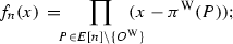
• (A) the normalized n-th division polynomial is

  

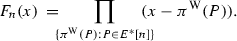
• (B) the normalized n-th primitive division polynomial is

  

Theorem 2.2

We have the following explicit formulas:

• (A)
  

  the degree and the first three coefficients are

  
• (B)
  

  the degree and the first three coefficients are

  

  where

  $$\begin{aligned} I(n)={\left\{ \begin{array}{ll} \,2 &{}\quad if \quad n=2,\\ \,1 &{}\quad if \quad n>2, \end{array}\right. } \end{aligned}$$

  and

  

  is Jordan’s totient function.

Proof

(A)  Notice that $f_{n}(x)=\psi _{n}^{2}(x)/n^{2}$, so the inductive formulas for $\psi _{n}$ can be transformed to

$$\begin{aligned} f_{2n+1} = \biggl (\frac{n^{3}(n+2)}{2n+1}\,\sqrt{f_{n}^{3}f_{n+2}}-\frac{(n-1)(n+1)^{3}}{2n+1}\,\sqrt{f_{n-1}f_{n+1}^{3}}\biggr )^{2} \end{aligned}$$

for $n\geqslant 2$, and

$$\begin{aligned} f_{2n} = \biggl (\frac{(n-1)^{2}(n+2)}{4}\,\sqrt{\frac{f_{n-1}^{2}f_{n}f_{n+2}}{f_{2}}}-\frac{(n-2)(n+1)^{2}}{4}\,\sqrt{\frac{f_{n-2}f_{n}f_{n+1}^{2}}{f_{2}}}\biggr )^{\!2} \end{aligned}$$

for $n\geqslant 3$. In order to use induction to prove the formulas for $t(n)=d(n)$, $c_{1,0,0}(n)$, $c_{0,1,0}(n)$, and $c_{0,0,1}(n)$, we need to check the initial values t(n) for $1\leqslant n\leqslant 4$, and verify that they all satisfy

for $n\geqslant 2$, and

for $n\geqslant 3$. All of these can be easily done.

(B)  By definition,

so for $T(n)=D(n)$, $C_{1,0,0}(n)$, $C_{0,1,0}(n)$, and $C_{0,0,1}(n)$, we have

Then the rest is a standard application of the Möbius inversion formula.$\square$

Theorem 2.3

Let $E_{1}$ and $E_{2}$ be two elliptic curves in the generalized Weierstrass form, then the following are equivalent:

• (A) $b_{i}(E_{1})=b_{i}(E_{2})$, $i=2,4,6$;

• (B) for any n, ;

• (C) $\pi ^\mathrm{W}(E_{1}[\infty ])=\pi ^\mathrm{W}(E_{2}[\infty ])$;

• (D) $\pi ^\mathrm{W}(E_{1}[\infty ])\cap \pi ^\mathrm{W}(E_{2}[\infty ])$ is infinite;

• (E) for some $n>1$, ;

• (F) for some $n_{1},\ldots ,n_{k}>1$, .

Proof

(A) $\Rightarrow$ (B) $\Rightarrow$ (C) $\Rightarrow$ (D) $\Rightarrow$ (E) $\Rightarrow$ (F) is clear, where (D) $\Rightarrow$ (E) is given by Theorem 1.1. Assume (F), then $E_{1}$ and $E_{2}$ share the same . Since $C_{1,0,0}(n)$, $C_{0,1,0}(n)$, and $C_{0,0,1}(n)$ are all strictly positive, the coefficients of $b_{2},b_{4}$, and $b_{6}$ in the product will always be nonzero, then $b_{2},b_{4}$, and $b_{6}$ can be solved, which proves (A).$\square$

Now let us go back to the general $(E,O,\pi )$, and assume that $\pi (O)=\infty$. By the Riemann–Roch theorem, there exists an isomorphism $\phi :E\rightarrow E'$ such that $E'$ is in the generalized Weierstrass form. Then $\phi$ induces fixing $\infty$, which must be a linear function [5]. Its inverse $\overline{\phi }{}^{\,-1}$ can be lifted to such that $E''$ remains in the generalized Weierstrass form. Thus the general case can be reduced to the Weierstrass case. Note that we can make everything above defined over K, except possibly $\widehat{\phi }$ has to be defined over a quadratic extension of K.

Corollary 2.4

Given $(E_{1},O_{1},\pi _{1})$ and $(E_{2},O_{2},\pi _{2})$ such that $\pi _{1}(O_{1})=\pi _{2}(O_{2})$, then the following are equivalent:

• (A) for any n, ;

• (B) for some $n>1$, ;

• (C) for some $n_{1},\ldots ,n_{k}>1$,;

• (D) $\pi _{1}(E_{1}[\infty ])=\pi _{2}(E_{2}[\infty ])$;

• (E) $\pi _{1}(E_{1}[\infty ])\cap \pi _{2}(E_{2}[\infty ])$ is infinite.

Proof

First move $\pi _{1}(O_{1})$ and $\pi _{2}(O_{2})$ to $\infty$ by a common fractional linear transformation, and then use the above argument.$\square$

The following corollary gives the converse of Theorem 1.1.

Corollary 2.5

Given $(E_{1},O_{1},\pi _{1})$ and $(E_{2},O_{2},\pi _{2})$, then the following are equivalent:

• (A) $\pi _{1}(E_{1}[2])=\pi _{2}(E_{2}[2])$;

• (B) $\pi _{1}(E_{1}[\infty ])=\pi _{2}(E_{2}[\infty ])$;

• (C) $\pi _{1}(E_{1}[\infty ])\cap \pi _{2}(E_{2}[\infty ])$ is infinite.

Proof

Assume (A), if $\pi _{1}(O_{1})=\pi _{2}(P)$ for some $P\in E_{2}[2]$, then the translation-by-P map $[+P]$ acts on $E_{2}[2]$ and $E_{2}[\infty ]$ bijectively, the projection map satisfies , which implies (B), by Corollary 2.4. (B) $\Rightarrow$ (C) is obvious, and (C) $\Rightarrow$ (A) is a restatement of Theorem 1.1.$\square$

Given Theorem 2.3, it is natural to ask

Question 2.6

Let $E_{1}$ and $E_{2}$ be two elliptic curves in the generalized Weierstrass form, if , can we always conclude that $n_{1}=n_{2}$?

If Conjecture 1.2 is true, then the answer must be yes, at least when $n_{1}$ and $n_{2}$ are large enough. A naive attempt is to write their division polynomials more explicitly, and then compare those coefficients. Clearly, a necessary condition is $D(n_{1})=D(n_{2})$. However, since we have, for example,

$$\begin{aligned} D(5)&=D(6)=12,\\ D(35)&=D(40)=D(42)=576,\\ D(55)&=D(57)=D(62)=D(66)=1440, \end{aligned}$$

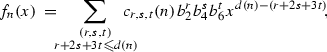
D(n) itself does not give a strong restriction on n. Notice that $C_{1,0,0}(n)=D(n)/12$, so $b_{2}(E_{1})=b_{2}(E_{2})$, we can assume the common value is 0, and consequently $b_{2}$ disappears in the formulas of $f_{n}(x)$ and $F_{n}(x)$. Based on the same approach as before, together with a tedious calculation, we can obtain all the coefficients $C_{0,s,t}(n)$ for $2s+3t\leqslant 6$.

Theorem 2.7

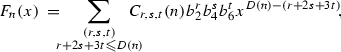
We have the following explicit formulas for the coefficients of $F_{n}(x)$:

$$\begin{aligned} C_{0,2,0}(n) =&-\biggl (\frac{1}{16800}\,J_{8}(n)+\frac{1}{600}\,J_{4}(n)+\frac{5}{672}\,J_{2}(n)\biggr )\,I(n)\\&+\frac{1}{2}\,\biggl (\frac{1}{120}\,J_{4}(n)+\frac{1}{24}\,J_{2}(n)\biggr )^{\!2}I^{2}(n),\\C_{0,1,1}(n) =&-\biggl (\frac{1}{92400}\,J_{10}(n)+\frac{1}{2800}\,J_{6}(n)+\frac{1}{1680}\,J_{4}(n)+\frac{1}{150}\,J_{2}(n)\biggr )\,I(n)\\&+\biggl (\frac{1}{120}\,J_{4}(n)+\frac{1}{24}\,J_{2}(n)\biggr )\biggl (\frac{1}{840}\,J_{6}(n)+\frac{1}{60}\,J_{2}(n)\biggr )\,I^{2}(n),\\ C_{0,0,2}(n) =&-\biggl (\frac{1}{1345344}\,J_{12}(n)+\frac{1}{7840}\,J_{6}(n)+\frac{1}{660}\,J_{2}(n)\biggr )\,I(n)\\&+\frac{1}{2}\,\biggl (\frac{1}{840}\,J_{6}(n)+\frac{1}{60}\,J_{2}(n)\biggr )^{\!2}I^{2}(n),\\ C_{0,3,0}(n) =&\; \biggl (\frac{1}{2574000}\,J_{12}(n)+\frac{1}{42000}\,J_{8}(n)+\frac{17}{36000}\,J_{4}(n)+\frac{5}{2464}\,J_{2}(n)\biggr )\,I(n)\\&-\biggl (\frac{1}{16800}\,J_{8}(n)+\frac{1}{600}\,J_{4}(n)+\frac{5}{672}\,J_{2}(n)\biggr )\\&\cdot \biggl (\frac{1}{120}\,J_{4}(n)+\frac{1}{24}\,J_{2}(n)\biggr )\,I^{2}(n)\\&+\frac{1}{6}\,\biggl (\frac{1}{120}\,J_{4}(n)+\frac{1}{24}\,J_{2}(n)\biggr )^{\!3}I^{3}(n). \end{aligned}$$

Proof

When n is odd, write

For this case, McKee [8] proved the following recurrence relation for $\widetilde{c}_{s,t}(n)$:

By this formula, we can first calculate $\widetilde{c}_{s,t}(n)$, and then $C_{0,s,t}(n)$. The case when n is even can be similarly dealt with another relation which is proved in the same paper.$\square$

Remark 2.8

Clearly, these formulas have some beautiful patterns, which we expect are shared by all $C_{r,s,t}(n)$. Specifically, depending on (r, s, t), each $C_{r,s,t}(n)$ is an alternating sum of several components, each component is a product of several subcomponents, and each subcomponent is a positive rational linear combination of $J_{k}(n)$.

If $j(E_{1}),j(E_{2})\ne 0,1728$, it suffices to show that the map

is injective. Unfortunately, although it is supported by extensive calculations, we fail to prove it. On the other hand, we have

Theorem 2.9

Let $E_{1}$ and $E_{2}$ be two elliptic curves in the generalized Weierstrass form such that for some $n_{1}\ne n_{2}$, then .

Proof

We have assumed $b_{2}=0$, so $j=0$ if and only if $b_{4}=0$, and $j=1728$ if and only if $b_{6}=0$. Since , we have

Thus there are three cases:

(A) $b_{4}(E_{1})=b_{4}(E_{2})=0$.  We can assume $b_{6}(E_{1}),b_{6}(E_{2})\in \mathbb {Q}^{{\times }}$, then $E_{1}$ and $E_{2}$ are both elliptic curves with complex multiplication by $\mathscr {O}_{L}$, the integer ring of . By class field theory [9] of imaginary quadratic fields [12],

is the ray class field of L for the modulus $n_{i}$. We want to determine all $\mathfrak {m}\ne \mathfrak {n}$ such that $L^{\mathfrak {m}}=L^{\mathfrak {n}}$. Since the common divisors of $\mathfrak {m}$ and $\mathfrak {n}$ give the same ray class field, it is enough to assume that , thus

so the indices

In L, 2 is inert, $3=\mathfrak {p}_{3}^{2}$ is ramified, and $7=\mathfrak {p}_{7a}\mathfrak {p}_{7b}$ splits. Then

$$\begin{aligned} I_{L}^{\mathfrak {m}}\cap L^{\times }= {\left\{ \begin{array}{ll} \,\mu _{6} &{} \quad \text {if}\quad \mathfrak {m}=1,\\ \,\mu _{3} &{}\quad \text {if}\quad \mathfrak {m}=\mathfrak {p}_{3},\\ \,\mu _{2} &{} \quad \text {if}\quad \mathfrak {m}=2,\\ \,\mu _{1} &{} \quad \text {otherwise,} \end{array}\right. } \end{aligned}$$

where $\mu _{N}$ is the group of N-th roots of unity, and

We conclude that different moduli give different ray class fields except for

$$\begin{aligned} L^{1}=L^{2}=L^{\mathfrak {p}_{3}}=L^{2\mathfrak {p}_{3}}=L^{\mathfrak {p}_{7a}}=L^{\mathfrak {p}_{7b}}. \end{aligned}$$

Thus the conductor of $L^{n}$ is n / I(n), $L^{n_{1}}=L^{n_{2}}$ implies $n_{1}=n_{2}$.

(B) $b_{6}(E_{1})=b_{6}(E_{2})=0$.  We can assume $b_{4}(E_{1}),b_{4}(E_{2})\in \mathbb {Q}^{\times }$, then $E_{1}$ and $E_{2}$ are both elliptic curves with complex multiplication by $\mathscr {O}_{L}$, the integer ring of . By class field theory of imaginary quadratic fields,

is the ray class field of L for the modulus $n_{i}$. In L, $2=\mathfrak {p}_{2}^{2}$ is ramified, and $5=\mathfrak {p}_{5a}\mathfrak {p}_{5b}$ splits. Then

$$\begin{aligned} I_{L}^{\mathfrak {m}}\cap L^{\times }= {\left\{ \begin{array}{ll} \,\mu _{4} &{} \quad \text {if}\quad \mathfrak {m}=1,\mathfrak {p}_{2},\\ \,\mu _{2} &{}\quad \text {if}\quad \mathfrak {m}=2,\\ \,\mu _{1} &{} \quad \text {otherwise,} \end{array}\right. } \end{aligned}$$

and

We conclude that different moduli give different ray class fields except for

Thus the conductor of $L^{n}$ is n / I(n), $L^{n_{1}}=L^{n_{2}}$ implies $n_{1}=n_{2}$.

(C) $b_{4}(E_{1}),b_{4}(E_{2}),b_{6}(E_{1}),b_{6}(E_{2})\ne 0$.  The relation

implies

Now $b_{6}^{2}(E_{1})/b_{4}^{3}(E_{1})\in \overline{\mathbb {Q}}$ unless all coefficients are zero. Part (B) implies that

as polynomials, so there exists some s such that

which in turn implies the constant term

Thus $b_{6}^{2}(E_{1})/b_{4}^{3}(E_{1})\in \overline{\mathbb {Q}}$, which implies $j(E_{1}),j(E_{2})\in \overline{\mathbb {Q}}$.$\square$

3 Intersection of projective torsion points

Now let K be a number field, the absolute Galois group of K,

the cyclotomic character of K. Consider the associated Galois representation

Since , we always have . Zywina [16] proved that if $K\ne \mathbb {Q}$, then for almost all elliptic curves defined over K, this is actually an equality, namely, .

Theorem 3.1

Given $(E_{1},O_{1},\pi _{1})$ and $(E_{2},O_{2},\pi _{2})$, all defined over a number field $K\ne \mathbb {Q}$, if

• (A) $\pi _{1}(O_{1})=\pi _{2}(O_{2})$,

• (B) Corollary 2.4 does not hold,

• (C) ,

then $\#\,\pi _{1}(E_{1}[\infty ])\cap \pi _{2}(E_{2}[\infty ])=1$.

Proof

Suppose that there exists for some $n_{1},n_{2}>1$. By assumption (C), $G_{K^\mathrm{cyc}}$ transitively acts on , which is therefore the orbit of a, and the degree of a is given by $D(n_{i})$. We also have the exact sequence

as a consequence,

which implies that $n_{1}=n_{2}$, hence contradicts (A) and (B).$\square$

For any $\sigma \in G_{K}$, $\sigma (\sqrt{\mathrm{\Delta }})=\epsilon (\rho _{E}(\sigma ))\sqrt{\mathrm{\Delta }}$, where

is the signature character. If $K=\mathbb {Q}$, then $\sqrt{\mathrm{\Delta }}\in \mathbb {Q}^{ab}=\mathbb {Q}^\mathrm{cyc}$, so , a subgroup of index 2 in . Jones [6] proved that for almost all elliptic curves defined over $\mathbb {Q}$, this is actually an equality, namely, .

Theorem 3.2

Given $(E_{1},O_{1},\pi _{1})$ and $(E_{2},O_{2},\pi _{2})$, all defined over $\mathbb {Q}$, if

• (A) $\pi _{1}(O_{1})=\pi _{2}(O_{2})$,

• (B) Corollary 2.4 does not hold,

• (C) ,

then $\#\,\pi _{1}(E_{1}[\infty ])\cap \pi _{2}(E_{2}[\infty ])=1$.

Proof

The proof is nearly the same as the case $K\ne \mathbb {Q}$, except that

If $n_{1}\ne n_{2}$, then $n_{1}=n_{2}/2$ is odd, which implies $D(n_{1})=D(n_{2})/3$, a contradiction. $\square$

Remark 3.3

If Question 2.6 has an affirmative answer, then assumption (C) in Theorems 3.1 and 3.2 can be weakened by assuming that $G_{K}$ acts on transitively. This suggests that our Conjecture 1.2, apparently an unlikely intersection type problem [15], might be somewhat related to Serre’s uniformity conjecture [11].

With the condition $\pi _{1}(O_{1})=\pi _{2}(O_{2})$ dropped, more intersection points can be obtained. We begin with the classical results for 3-torsion points and 4-torsion points.

Proposition 3.4

For any elliptic curve E defined over K, there exists an even morphism $\pi \in \overline{K}(E)$ of degree 2 such that , where $\rho$ is a primitive cube root of unity.

Proof

Consider the family $E_{\lambda }:x^{3}+y^{3}+z^{3}=3\lambda xyz$, which is an elliptic curve provided $\lambda ^{3}\ne 1$. Its 3-torsion points are

If we take the origin to be , then the projection map $\pi _{\lambda }:E_{\lambda }\rightarrow \mathbb {P}^{1}$, maps $E_{\lambda }^{*}[3]$ to the desired set. Since every elliptic curve defined over K can be transformed to some $E_{\lambda }$ via an isomorphism defined over $\overline{K}$, the conclusion follows.$\square$

Proposition 3.5

For any elliptic curve E defined over K, there exists an even morphism $\pi \in \overline{K}(E)$ of degree 2 such that , where i is a primitive fourth root of unity.

Proof

Consider the family , which is a curve of genus 1 with a unique singularity at provided $\delta ^{4}\ne 0,1$. Its 2-torsion points respectively induce if we take $O_{\delta }=(\delta ,0)$, and $\pi _{\delta }:E_{\delta }\rightarrow \mathbb {P}^{1}$, $(x,y)\mapsto x$. The fixed points of those nontrivial ones, $\{0,\infty \}$, and , therefore constitute the collection of $\pi _{\delta }(E_{\delta }^{*}[4])$. Since every elliptic curve defined over K can be transformed to some $E_{\delta }$ via a birational isomorphism defined over $\overline{K}$, the conclusion follows.$\square$

Propositions 3.4 and 3.5 indicate that for any elliptic curve, the projective 3-torsion points are equivalent to the vertices of a regular tetrahedron, while the projective 4-torsion points are equivalent to the vertices of a regular octahedron. It is therefore tempting to guess the projective 5-torsion points are equivalent to the vertices of a regular icosahedron. However, this is not the case. Following Klein [7], consider the family

Its projective 5-torsion points can be explicitly expressed as

where $\omega$ is a primitive fifth root of unity, and $k\in \mathbb {Z}/5\mathbb {Z}$. Since the cross ratio

is not a constant, the projective 5-torsion points are not equivalent to any fixed collection of 12 points.

Although any single $\pi (E^{*}[2]),\pi (E^{*}[3])$, or $\pi (E^{*}[4])$ is insufficient to determine $\pi (E[\infty ])$, any pair of them can do so.

Corollary 3.6

Given $(E_{1},O_{1},\pi _{1})$ and $(E_{2},O_{2},\pi _{2})$, if

• (A) $\pi _{1}(E_{1}^{*}[2])=\pi _{2}(E_{2}^{*}[2])$ and $\pi _{1}(E_{1}^{*}[3])=\pi _{2}(E_{2}^{*}[3])$, or

• (B) $\pi _{1}(E_{1}^{*}[2])=\pi _{2}(E_{2}^{*}[2])$ and $\pi _{1}(E_{1}^{*}[4])=\pi _{2}(E_{2}^{*}[4])$, or

• (C) $\pi _{1}(E_{1}^{*}[3])=\pi _{2}(E_{2}^{*}[3])$ and $\pi _{1}(E_{1}^{*}[4])=\pi _{2}(E_{2}^{*}[4])$,

then $\pi _{1}(O_{1})=\pi _{2}(O_{2})$. In particular, Corollary 2.4 holds.

Proof

(A)  It suffices to show that $\pi (E^{*}[2])$ and $\pi (E^{*}[3])$ determine $\pi (O)$. By Proposition 3.4, we can assume . Let $\lambda =\pi (O)$, and consider $(E_{\lambda },O_{\lambda },\pi _{\lambda })$. Since

we have $\pi _{\lambda }(O_{\lambda })=\lambda$. By Corollary 2.4, $\pi _{\lambda }(E_{\lambda }^{*}[2])=\pi (E^{*}[2])$. Thus we just need to show that $\pi _{\lambda }(E_{\lambda }^{*}[2])$ determines $\lambda$. Since the points in $\pi _{\lambda }(E_{\lambda }^{*}[2])$ are the roots of $x^{3}+3\lambda x^{2}-4$, this is clear.

(B)  determines $\delta$.

(C)  We need to show that $\pi _{\delta }(E_{\delta }^{*}[3])$ determines $\delta$. The nonsingular model of $E_{\delta }$ is

$$\begin{aligned} E_{\delta }^{ns}:\; Y^{2}=X(X-1)\biggl (X-\frac{1}{4}\biggl (\delta +\frac{1}{\delta }\biggr )^{2}\biggr ), \end{aligned}$$

where

The division polynomials of $E_{\delta }^{ns}$ imply the division polynomials of $E_{\delta }$ via this birational isomorphism. In particular, the points in $\pi _{\delta }(E_{\delta }^{*}[3])$ are the roots of , then the result is immediate.$\square$

Now we are ready to give the main result of this article. For any $E_{\delta _{1}}$ and $E_{\delta _{2}}$, the intersection of $\pi _{\delta _{1}}(E_{\delta _{1}}[\infty ])$ and $\pi _{\delta _{2}}(E_{\delta _{2}}[\infty ])$ has at least six elements. If it contains another element a, then as we have seen in the proof of Proposition 3.5, it also contains , 1 / a, and . Therefore, its cardinality must be $4k+6$. If we fix $\delta _{1}$ and vary $\delta _{2}$, then $k=1$ can be easily attained. In the next theorem, we construct an example to improve $k=2$.

Theorem 3.7

$\sup {(\#\,\pi _{1}(E_{1}[\infty ])\cap \pi _{2}(E_{2}[\infty ]))}\geqslant 14$, where supremum is taken over $(K,E_{1},O_{1},\pi _{1},E_{2},O_{2},\pi _{2})$ such that $\pi _{1}(E_{1}[2])\ne \pi _{2}(E_{2}[2])$.

Proof

From the division polynomials of $E_{\delta }^{ns}$, we know that the third and fifth primitive division polynomials of $E_{\delta }$ are

Now we want to find $\delta _{1}$ and $\delta _{2}$ such that there exist $u\in \pi _{\delta _{1}}(E_{\delta _{1}}^{*}[3])\cap \pi _{\delta _{2}}(E_{\delta _{2}}^{*}[3])$, and $v\in \pi _{\delta _{1}}(E_{\delta _{1}}^{*}[5])\cap \pi _{\delta _{2}}(E_{\delta _{2}}^{*}[5])$. In other words, , and . Since is a quadratic polynomial in $\delta$, any fixed u such that $u^{4}\ne 0,1$, and $u^{8}+14u^{4}+1\ne 0$ gives exactly two roots satisfying $\delta _{1}^{4},\delta _{2}^{4}\ne 0,1$, and . Since $\delta _{1}$ and $\delta _{2}$ are also two roots of , we have as polynomials in $\delta$. By long division, this is equivalent to require

Consider $C_{0}$ and $C_{1}$ as polynomials in v, then their resultant is

whose roots are the u-coordinates of their common points. Let u such that $u^{4}\ne 0,1$ be any nontrivial root, (u, v) the corresponding common point, $\delta _{1}$ and $\delta _{2}$ the roots of , then we have

so the supremum is at least 14.$\square$

Remark 3.8

After submitting this article, we have successfully improved the previous result from 14 points (using 3-torsion points and 5-torsion points) to 22 points (using 3-torsion points and 7-torsion points). We will give full details in the next publication.

Remark 3.9

The intersection can also be investigated using Tate’s explicit parametrization of elliptic curves over p-adic fields [12]. We plan to explore the details of this approach in the future.

4 Appendix: Jordan’s totient function

We are concerned with the values taken by $J_{k}(n)$ as well. $J_{1}(n)$ is simply Euler’s totient function, for which we have the famous Ford’s theorem [4] and Carmichael’s conjecture [2, 3]. $J_{2}(n)$ is far from being injective, which prevents a simple answer to Question 2.6. Even their combination is not injective, since

$$\begin{aligned} J_{1}(15)=J_{1}(16)=8,\qquad J_{2}(15)=J_{2}(16)=192. \end{aligned}$$

It is quite surprising that $J_{3}(n)$ is still not injective, the smallest identical pair is

$$\begin{aligned} J_{3}(28268)=J_{3}(28710)=19764446869440. \end{aligned}$$

We do not know any identical pair for $k\geqslant 4$, and expect that such coincidence should be very rare.

Finally, let us conclude this article with a collection of partial results:

Proposition 4.1

Let $p,q,p_{1}\ne p_{2}$, $q_{1}\ne q_{2}$ be primes, $v_{p}(n)$ the power of p in the prime decomposition of n, $\omega (n)$ the number of distinct prime divisors of n, then

• (A) If $J_{2}(p^{s})=J_{2}(q^{t})$, then $p^{s}=q^{t}$ or $\{p^{s},q^{t}\}=\{7,8\}$.

• (B) If $J_{k}(p_{1}p_{2})=J_{k}(q_{1}q_{2})$, $k=2,4$, then $p_{1}p_{2}=q_{1}q_{2}$.

• (C) If $J_{k}(m)=J_{k}(n),k=2,4,6$, then $v_{p}(m)=v_{p}(n)$ for $p=2,3$, $v_{p}(m)=v_{p}(n)$ or for any other $p\not \equiv 1 mod 12$, and $\omega (m)=\omega (n)$.

• (D) If $J_{k}(m)=J_{k}(n)$ for infinitely many k, then $m=n$.

Proof

(A)  Now we have . If $p,q\ne 2$ and $s,t\ne 1$, then p (resp. q) is the largest prime divisor of left-hand side (resp. right-hand side). Hence $p=q$ and $s=t$. If $p=2$, then . Since 4 cannot be a common divisor of $q+1$ and $q-1$, one of them must be a divisor of 6. Hence $q=2$ and $s=t$, or . If $s=1$, then . We can assume $q\ne 2$, then q cannot be a common divisor of $p+1$ and $p-1$, so , so $t=1$ and $p=q$, or $t=2$. If $t=2$, then either or , neither is possible.

(B)  It is straightforward that $(p_{1}^{2}-1)(p_{2}^{2}-1)=(q_{1}^{2}-1)(q_{2}^{2}-1)$ and $(p_{1}^{4}-1)$ $\cdot (p_{2}^{4}-1)=(q_{1}^{4}-1)(q_{2}^{4}-1)$ imply $p_{1}p_{2}=q_{1}q_{2}$.

(C)  Since , from , we can see $v_{2}(m)=v_{2}(n)$ or . Since , from , we can see $v_{3}(m)=v_{3}(n)$ or . This strategy works for any other $p\not \equiv 1\text { mod }12$, since either or is a quadratic nonresidue. If $v_{2}(m)=0$ and $v_{2}(n)=1$, then , a contradiction. If $v_{3}(m)=0$ and $v_{3}(n)=1$, then $5/4=$ , again a contradiction. Moreover, since , but , from $J_{4}(n)/J_{2}(n)$, we can see $\omega (m)=\omega (n)$.

(D)  Assume $k>1$, then , thus by symmetry. Since as $k\rightarrow \infty$, we have $m=n$.$\square$

References

Bogomolov, F., Tschinkel, Yu.: Algebraic varieties over small fields. In: Zannier, U. (ed.) Diophantine Geometry. CRM Series, vol. 4, pp. 73–91. Edizioni della Normale, Pisa (2007)
Carmichael, R.D.: On Euler’s \(\phi \)-function. Bull. Amer. Math. Soc. 13(5), 241–243 (1907)
Carmichael, R.D.: Note on Euler’s \(\varphi \)-function. Bull. Amer. Math. Soc. 28(3), 109–110 (1922)
Ford, K.: The number of solutions of \(\phi (x)=m\). Ann. Math. 150(1), 283–311 (1999)
Hartshorne, R.: Algebraic Geometry. Graduate Texts in Mathematics, vol. 52. Springer, New York (1977)
Jones, N.: Almost all elliptic curves are Serre curves. Trans. Amer. Math. Soc. 362(3), 1547–1570 (2010)
Klein, F.: Lectures on the Icosahedron and the Solution of Equations of the Fifth Degree, 2nd edn. Dover, New York (1956)
McKee, J.: Computing division polynomials. Math. Comput. 63(208), 767–771 (1994)
Neukirch, J.: Class Field Theory. Grundlehren der Mathematischen Wissenschaften, vol. 280. Springer, Berlin (1986)
Raynaud, M.: Courbes sur une variété abélienne et points de torsion. Invent. Math. 71(1), 207–233 (1983)
Serre, J.-P.: Propriétés galoisiennes des points d’ordre fini des courbes elliptiques. Invent. Math. 15(4), 259–331 (1972)
Silverman, J.H.: Advanced Topics in the Arithmetic of Elliptic Curves. Graduate Texts in Mathematics, vol. 151. Springer, New York (1994)
Silverman, J.H.: The Arithmetic of Elliptic Curves. Graduate Texts in Mathematics, vol. 106, 2nd edn. Springer, Dordrecht (2009)
Wolfram Research, Inc. Mathematica, Version 10.0. Champaign, IL (2014)
Zannier, U.: Some Problems of Unlikely Intersections in Arithmetic and Geometry. Annals of Mathematics Studies, vol. 181. Princeton University Press, Princeton (2012)
Zywina, D.: Elliptic curves with maximal Galois action on their torsion points. Bull. London Math. Soc. 42(5), 811–826 (2010)
Author information
Authors and Affiliations
Corresponding author
Additional information
The first author acknowledges that the article was prepared within the framework of a subsidy granted to the HSE by the Government of the Russian Federation for the implementation of the Global Competitiveness Program. The first author was also supported by a Simons Travel Grant. The second author was supported by the MacCracken Program offered by New York University.
Rights and permissions
About this article
Cite this article
Bogomolov, F.A., Fu, H. Division polynomials and intersection of projective torsion points. European Journal of Mathematics 2, 644–660 (2016). https://doi.org/10.1007/s40879-016-0111-7
Received:
Revised:
Accepted:
Published:
Issue Date:
DOI: https://doi.org/10.1007/s40879-016-0111-7