
Abstract
The advent of smart grid is a revolution that has enabled power distribution in a more efficient way. However, load forecasting, demand response management and accurate consumer load profiling using smart meter data continue to be challenging industry and research problems. Clustering is an efficient technique for load profiling. K-means clustering algorithm for clustering electricity consumers based on raw meter data directly result in cumbersome, redundant and inefficient computations. This paper presents a methodology for reducing the raw data set dimension via features extraction and cluster the load profiles based on computed features. The feature set formed comprises of Singular Values by Singular Value Decomposition and Wavelet Energy Entropy of approximate and detailed Coefficients. K means Clustering technique is used. The proposed method enables efficient and quick clustering and at the same time the information content in load profiling is preserved. The time consumed for clustering of feature set formed is found to be much less than that of raw data set. By comparing the Silhouette Values K = 6 was found to be the optimal number of clusters with average silhouette coefficient around 0.79. Clustering of load profiles both for Raw Data Set as well as computed Feature Set are compared by evaluating average silhouette value, number of negative silhouettes and computation time for clustering and Silhouette Coefficient was found to be 0.79 by proposed methodology showing better clustering result as compared to raw dataset.
Introduction
An electricity network with advanced digital technology and two way communication forms the smart grid which has taken energy industry to a higher level. This is the need of time due to depleting resources, deteriorating environmental conditions and escalating energy demand [1]. One of the most important component of smart grid are smart meters. They are advanced energy meters that provide high frequency energy consumption data from the end user’s load devices to the utility company with some added information. These meters allows two way communication of information between users and utilities which helps consumers to make informed energy choices. For harnessing maximum information from the data provided by smart meters, analysis and processing of data is one of the most important step.
In this paper the analysis of residential and small enterprises consumer smart meter data is done to understand the variation in load profile of various consumers at different time intervals. This helps the Distribution Network Operators (DNO) to identify suitable candidates for demand response management. It also helps DNOs to understand the energy behaviour of different types of consumers and improve the modelling of overall energy profile [2]. The consumer end demand is highly stochastic and irregular, hence detailed analysis is required [3].
The load profiles obtained from electricity consumption data are clustered into different groups based on the evaluated attributes from smart meter data with the inclusion of Time of Use (ToU) [4]. This is done to identify consumers with heavy usage during peak demand time. If dynamic tariffs are introduced, informed consumers will shift their usage from peak load time to off peak time and hence assist in flattening the energy load demand curve [5]. But clustering the raw data from smart meters takes more time hence it is necessary to extract the key features from the dataset (to reduce the redundancy and increase the efficiency of process) [2].
Literature Review
The large amount of data from smart meters over short duration of time is providing researchers with deeper insight into the consumer energy use pattern. Analysing this data will help the power companies in areas like demand response management, load forecasting, power quality monitoring and event detection [4, 8, 24].
In order to determine the eligible consumers for demand response programmes, the normalised weekday load profiles are clustered in [11]. Four clustering techniques, i.e., random forest approach, k- Nearest Neighbour, decision tree and artificial neural network, are compared and it is found that random forest clustered the data better than others. But due to high computational cost and redundancy in data, instead of using raw data, extraction of salient features is considered an important step before clustering [2] [4,5,6,7,8,9,10] [12,13,14]. Features can be found in time [2] [7, 8] [13], frequency [8] and time frequency [9] domains in order to have better knowledge about characteristics of meter data. The smart meter data is divided into four key time periods in [2] for capturing the peak load and major sources of variability in a day. Seven statistical features were found in each time period for clustering. Due to weak correlation between different features, finite mixture model technique was used for clustering the data into 10 unique clusters. The optimal number of clusters was chosen by Bayesian Information Criterion and to check robustness of model, bootstrapping was used. When analysing data from many smart meters, clustering can be done in two stages as shown in [6]. In first stage the pattern variability was captured and clustered for each user individually and then in second stage these clusters were combined to find global clusters. Comparison of k-means and g-means clustering techniques was done based upon the coefficients found by fast wavelet transform (using haar wavelet). The number of clusters formed in this method are very high as compared to other work in literature which is not considered good. Feature extraction technique can also be used for classifying different types of disturbances in the signal as in [8]. Here, features are extracted in both time and frequency domain (using FFT) of synthetic signals, to determine the most relevant characteristics for off- line analysis of disturbances in power line. For classification of disturbances decision tree showed better performance as compared to artificial neural network. In [9] for extracting hidden electricity usage patterns, the data is decomposed into several partial usage patterns using K-SVD. This is done so that load gets compressed in sparse way. The advantage of using this technique is that there is no assumption required for base signal rather it learns them automatically. In this work, features from consumer load data are classified using linear SVM (supervised learning technique) into two classes i.e. residents and small and medium enterprises. Clustering techniques can also be used to estimate the load demand as shown in [10]. There, an algorithm based on k-means cluster analysis was applied on segmented load profiles (less than or equal to 24 h) of aggregated smart meters. The cluster centres along with various distance functions (Canberra, manhattan, Euclidean and pearson) were used to estimate missing and future values by using other data in the same cluster. For harvesting the inherent structure from smart meter data, autocorrelation was applied with 24 lags on one week smart meter data in [12]. Then k means clustering technique was used on reduced dataset and it was found that for 32,241 smart meter data (over a period of one week) the optimal number of clusters were 12 (found by evaluating DBI mean index). In [13] a novel approach for modelling smart meter data is proposed using clustering and linearization of smart meter data curves. After pre-processing the data, extended k means algorithm is applied for obtaining the patterns with similar energy consumption. The load profile in each cluster is averaged, smoothened and then linearized. Using Particle Swarm Optimization, the linearized load profile are optimized for classification.
The high frequency data obtained from numerous smart meters introduces challenges for communication, storage and analysis of load profiles of consumers. This leads to the need for introduction of dimensionality reduction of data in a way that the features which define the maximum information about the load curve are retained and remaining are removed [9, 14]. Choosing appropriate features for efficient clustering of consumer load profile is very important.
Contribution of the Paper
In this work analysis of smart meter data obtained over prolong period of time (approximately six months) is done. In literature most of the work focussed on feature extraction in only one domain; mostly time domain. But in this work features are extracted in both time and time-frequency domains for better understanding of the load profiles and to obtain unique set of features for efficient clustering. By graphical analysis of the load profiles it is found that they show similar characteristics on each day of week (i.e. all Monday’s show similar profiles over a period of atleast one month and so on) as shown in Fig. 3a, b. This might be due to similar type of power consumption on same day of week. Hence load profiles are grouped together over a month for feature extraction so that redundancy in the load profiles having similar characteristics is reduced.
Aim of this work is to cluster the load profiles in a way that the process takes minimum time and the clusters formed are well separated from each other. For redundancy reduction, singular value decomposition is applied on raw data set for feature extraction. Five features are found from smart meter data for reducing computational cost, dimensionality and redundancy in data while clustering. For this purpose K means clustering algorithm is applied on the feature set and results are evaluated by using three clustering performance parameters i.e. Silhouette coefficient, process time and number of negative silhouettes. The number of clusters are chosen accordingly. It is shown in table 1 that derived feature set takes much less time when compared with raw dataset for clustering the load profiles.
Structure
The remaining part of the paper is organized such that section II describes the methodology for feature extraction in both the time and time-frequency domains, and the clustering techniques used. Section III shows details about data set and evaluation and validation of the proposed methodology. In Section IV, results and discussion on clustering technique used is presented. Section V gives conclusions and scope for future work.
Methodology
The various steps taken for clustering of load profiles is shown with the help of block diagram in fig.1. After data acquisition and pre-processing of smart meter data, the aim is to extract features which gives maximum information about the signal with minimum dimension of the feature set. The feature set proposed in this method consists of singular values obtained by singular value decomposition (SVD) and wavelet energy entropy obtained by finding the entropy of the energy content of wavelet coefficients (both detailed and approximate). These features are clustered using K-means algorithm. To find out how well separated each cluster values are from the values in another cluster, silhouette coefficients are computed.

Block Diagram representation for clustering load profiles
Singular Value Decomposition (SVD)
The raw data set consisting of energy consumption of each consumer is quite large. Much of the information it contains is redundant hence it is required to extract relevant information from it. For this purpose Singular values are determined by carrying out Singular Value Decomposition for each set of data matrix. It acts as an excellent technique to process the data, reduce the dimensions and find hidden information of the signal [16]. Singular Value Decomposition decomposes a matrix A such that the resultant describes basic properties of A [16, 17]. If matrix A of size n*d is decomposed by Singular Value Decomposition, a product of three matrices is obtained –
Where columns of matrices U and V of size m*n and n*n respectively gives left and right singular vectors. The columns of these vectors are orthonormal Eigen vectors of ATA and AAT. S is a diagonal matrix of size n*n containing the singular values of the matrix A. Equation (1) can also be expressed as sum of rank 1 matrices as shown in eq. (2)–
Where ui and vi are the elements of matrices U and V and 휎i corresponds to the singular values. These values are arranged in descending order of their magnitude with most significant value being the highest [15]. The singular values are related to Eigen values of matrices ATA and AAT and gives an idea of relation between various elements of data matrix with it’s transpose matrix [14, 18].
Wavelet Energy Entropy
Discrete Wavelet Transformation (DWT) of a signal allows both time and frequency domain analysis using discretely sampled wavelets. It captures both frequency and location (in time) information. DWT decomposes a signal into different sub-bands on the basis of frequency, i.e., low frequency band and high frequency band [19].
The wavelet transform of signal arranged in the form of matrix A is found by convolving the elements of matrix with the low pass filter and the high pass filter to give approximate (cA1) and detail (cD1) wavelet coefficients after down-sampling as shown in fig. 2. With each step of wavelet decomposition, the approximate coefficients are further decomposed into sub-bands of low and high frequency coefficients. For example in this work signal is decomposed upto 3 levels hence cA1, cD1, cD2 and cD3 were obtained as wavelet coefficients.

Discrete Wavelet Transform upto first decomposition level
Now, to find the wavelet energy, each of these coefficients is squared and summed in each time stamp. These energies are used for finding wavelet energy entropy which is the measure of randomness or uncertainty of the wavelet energy signal [20]. Shannon defined information entropy [21] as follows which is used in this work to find wavelet energy entropy–.
If X is the sample space consisting of n samples and P is the probability of ith piece of information i.e. xi then the self-information of each sample xi is given by –logePi and its expected value gives the entropy of the information source as given by the following equation –
If probability of each event is same, then their uncertainty is maximum and hence their entropy. To find wavelet energy entropy, Pi is given by the relative wavelet energy which is the ratio of each energy term with the total energy.
Clustering
Clustering is a technique to partition the data (here load profiles) into groups such that number of load profiles are more than the number of clusters. Thus, the load profiles showing similar behaviour are grouped in same cluster in a way that the intra cluster similarity is maximum and inter cluster similarity is minimum [22]. In this work, K-means clustering technique is used which comes under partitional clustering analysis method. In K means clustering, data is divided into k discrete clusters by minimizing the Euclidean distance of each load profile characteristics from the cluster centre.
Clustering results are checked in this work by evaluating cluster productivity ratio and silhouette coefficient. Cluster Productivity Ratio is the ratio of number of output clusters with number of input profiles. It tells how less number of clusters are used for grouping the similar load profiles.
Silhouette Coefficient indicates how close samples of a cluster are to each other and how far are the samples from other clusters which is given by the following equation –
Here, ‘b’ is smallest average distance of a sample in one cluster from the samples in another cluster and ‘a’ is the smallest distance of this sample from the samples in its own cluster. It’s value lies between −1 and 1, with 1 indicating the best clustering and − 1 indicating wrong clustering.
Work Done
In this work the analysis of residential and small enterprises consumer smart meter data is done to understand the variation in load profile of various consumers at different time intervals.
Data Acquisition and Pre-Processing
Statistically robust smart meter data is required for analysis and design of a reliable clustering model. Hence, in this work, smart meter data from Irish Smart Meter Database is used [23]. Data of 40 customers over a period of half year (from 20 July 2009 to 13 January 2010) is taken. The aim of using data for prolong period of time is to obtain results that contain load profiles of consumers in varying environmental conditions. The readings are taken at half hourly intervals which accounts for 48 samples of energy consumption data throughout the day and 8544 samples over the specified period of time for a single consumer. For 40 smart meters the total samples are 3,41,760. The data obtained is arranged in a matrix such that each row vector represents load consumption of a customer over a day.
Feature Extraction
After pre-processing the data (removal of absurd values and matrix formation), the load profile of various consumers was plotted. Similar consumption behaviour was observed on same day of the week (i.e. all Mondays have similar load profile and so on) over a period of one month as shown in Fig. 3.

(a). Load profile of ID2040 on Tuesdays of week 5, 6, & 7; (b). Load profile of ID2030 on Tuesdays of week 6,7 & 8.
It was also observed that mainly load profile of a day can be divided into three key time periods based on the variation in their consumption pattern. In these time periods (with 16 samples each) relevant attributes were found for clustering –.
•Time period 1: 12:00 am to 8:00 am.
•Time period 2: 8:00 am to 4:00 pm.
•Time period 3: 4:00 pm to 12:00 am.
Practically the number of consumers is much higher and for clustering it is essential to find certain attributes from the raw data set that defines this data in best possible way. This is done so that best possible clusters are formed in minimum time. Therefore Singular Value Decomposition has been performed on the dataset to compute the singular values. For SVD the data of 178 days (arranged row wise) of a consumer was arranged in a matrix form and from this data singular values were found for each block of 4*16 samples where 4 represented all load profiles of a day of week for a period of one month (e.g. all Tuesdays over a month) and 16 samples were taken for each day at a time that included key time periods of a day.
SVD helps in reducing the matrix dimension by pushing the less significant rows to the bottom. It was found that there is a wide difference between first singular value and the remaining ones (as shown in fig. 4).

Singular Values of ID2030 for 1 time stamp
Hence only first singular value was taken as the key feature for clustering the load profiles as it contained maximum information. Almost negligible difference was observed in the clustering results on inclusion of other singular values hence they were excluded from the feature set in order to reduce feature set dimension and complexity.
Other features were computed in time-frequency domain. Wavelet transform of load profile was found upto 3 levels of decomposition in each time stamp. Figure 5 shows the coefficients obtained after wavelet decomposition of one of the consumers. Daubechies2 (db2) wavelet was used for decomposition as it is generally used to find closely spaced features. Energy and hence energy entropy of approximate and detailed coefficients was further evaluated.

Wavelet Decomposition of energy consumption of ID2030 upto 3 levels using db2 wavelet
The aim of evaluating features in time-frequency domain was to find randomness in signal due to both low frequency and high frequency coefficients. In this work all detailed and approximate coefficients were included in the feature set matrix for the calculation of energy entropy so that each band of frequency was taken into consideration.
As explained in the earlier sections similarity was observed in load profile of consumers on each day of the week for a period of month. Thus for each coefficient a single value of wavelet energy entropy was found for specified period of time. It reduces the redundancy in the feature set in a way that a single feature in each frequency band gives maximum information about the possible randomness in signal showing similar characteristic.
Figure 6 illustrates the plot of all features extracted for a single customer over a span of specified time period. Variations in each feature can be seen in peaks as well as pattern. Hence they all can be included for clustering.

Values of Maximum Singular Values, wavelet energy entropy (WEE) of approximate coefficient, WEE of detailed coefficient 1, WEE of detailed coefficient 2 and detailed coefficient 3 (arranged from top to bottom) of ID2030
Results obtained by clustering these features are presented in the next section.
Results and Discussions
For each customer 5 attributes in each time slot were calculated as shown in fig. 6. One of the attributes is the maximum singular value and the remaining four were obtained from wavelet energy entropy of coefficients. The feature matrix reduced the raw dataset from 3,41,760 samples to 25,200 samples in a way that maximum information required for clustering the load profiles was retained. For clustering these load profiles k means clustering technique was used. This clustering technique uses an iterative approach to reduce the sum of distance from each point to centroid for all k clusters. For evaluating the performance of the clustering technique chosen and for checking for optimal number of clusters various parameters i.e. Average Silhoutte Value, Computation Time for Clustering and Number of Negative Silhouttes as shown in Table 1 were computed. From Table 1 it can be clearly inferred that clustering the profiles by reducing the dimensionality (i.e. by evaluating key feature set) is a better and less time consuming approach as compared to clustering the raw data.
From Table 1 it can also be inferred that optimal number of clusters for a set of 40 houses is 6 as all the parameters are optimized. It can be seen that average silhouette value is close to 1 with lesser negatives for k = 6. This shows that the distance of sample from samples in its own cluster is lesser than that from samples in other clusters. The computation time for clustering is also less for k = 6.
Further, in Table 2 Cluster Productivity Ratio is found in order to find the compactness of the clusters. It is the ratio of number of clusters formed and number of profiles given as input. Lower value of cluster productivity ratio indicates that fewer clusters are required for grouping the load profiles. Hence, in this work, the cluster productivity ratio of two best cases (i.e. when number of clusters are 6 and 7) was compared and it was found that choosing k = 6 is showing better results.
The Silhouette plot obtained for two best clusters i.e. k = 6 and k = 7 are shown in Fig. 7 below. It could be clearly observed that for k = 6, the plot shows fewer negative values. This indicates most of the clusters formed are able to group the feature set of load profiles in a way that intra cluster distance is minimum and inter cluster separation is maximum. Hence, taking k = 6 to be the optimum value for clustering these load profiles.

Silhouette Plot for K-6 and K-7 respectively of the result obtained after clustering the feature set.
Conclusions
The advent of smart metering has enabled efficient load forecasting, demand response management and event detection. This paper proposes a method to analyse fine-grained smart meter data obtained from consumer electricity consumption. Five features are found from smart meter data for reducing computational cost, dimensionality and redundancy in data while clustering.
The singular values are obtained from SVD of raw data and WEE of detailed and approximation coefficients are the selected features as they capture maximum information content and randomness in data. These features are clustered by using k-means clustering algorithm as it is a simple and fast clustering technique. The focus of this paper is on reducing computational complexity, at the same time preserving the information content in load profiles and hence enable efficient and quick. It is found that clustering of features from smart meter data takes lesser time and shows better clustering as compared to clustering raw dataset. The clustering performance is found by evaluating Silhouette Coefficient and Cluster Productivity Ratio. For half yearly data of 40 consumers, it is found that k = 6 shows better performance.
In future, after clustering load profiles, it is intended to predict the load demand of consumer based on the cluster it falls in. The evaluated features will further be used for getting better insight of decomposed data by including singular vectors (U and VT) in the feature set. More features in all three domains (time, frequency and time-frequency) will be evaluated and compared for better analysis of the load profile by using different clustering techniques.
Apart from load profile segmentation, clustering techniques also assist in load forecasting, state estimation, load management like consumer characterization and demand response management etc. areas. These areas are the pressing issues for implementation of smart grid and may be taken into consideration in future.
-
1.
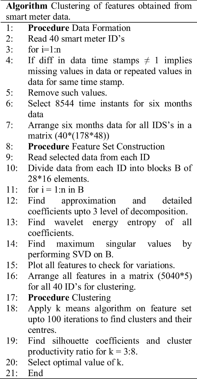
Algorithm

Abbreviations
- DNO:
-
Distribution Network Operator
- ToU:
-
Time of Use
- kSVD:
-
k Singular Value Decomposition
- SVM:
-
Support Vector Machine
- kNN:
-
k Nearest Neighbour
- ANN:
-
Artificial Neural Network
- SVD:
-
Singular Value Decomposition
- DWT:
-
Discrete Wavelet Transform
- cA1:
-
Approximation Coefficient
- cD1:
-
Detailed Coefficient
- db2:
-
Daubechies2
- WEE:
-
Wavelet Energy Entropy
References
Melzi F, Same A, Zayani M, Oukhellou L (2017) A Dedicated Mixture Model for Clustering Smart Meter Data: Identification and Analysis of Electricity Consumption Behaviours. Energies 10(10) https://pdfs.semanticscholar.org/d63f/a210852a22216566c9e9b84bc80d0e7c6a4c.pdf, Accessed on 10 Feb 2018
Haben S, Singleton C, Grindrod P (2016) Analysis and clustering of residential customers energy behavioral demand using smart meter data. IEEE Transactions on Smart Grid 7(1):136–144
De Souza J, Assis T, Pal B (2017) Data compression in smart distribution systems via singular value decomposition. IEEE Transactions on Smart Grid 8(1):275–284
Wang Y, Chen Q, Kang C, Zhang M (2015) Ke Wang and Yun Zhao, ‘load profiling and its application to demand response: a review’. Tsinghua Sci Technol 20(2):117–129
Azaza M, Wallin F (2017) Smart meter data clustering using consumption indicators: responsibility factor and consumption variability. Energy Procedia 142:2236–2242
Mets K, Depuydt F, Develder C (2016) Two-stage load pattern clustering using fast wavelet transformation. IEEE Trans Smart Grid 7(5):2250–2259
Al-Otaibi R, Jin N, Wilcox T, Flach P (2016) Feature construction and calibration for clustering daily load curves from smart-meter data. IEEE Trans Ind Informat 12(2):645–654
Borges F, Fernandes R, Silva I, Silva C (2016) Feature extraction and power quality disturbances classification using smart meters signals. IEEE Transactions on Industrial Informatics 12(2):824–833
Wang Y, Chen Q, Kang C, Xia Q, Luo M (2017) Sparse and redundant representation-based smart meter data compression and pattern extraction. IEEE Trans Power Syst 32(3):2142–2151
Al-Wakeel A, Wu J, Jenkins N (2017) K -means based load estimation of domestic smart meter measurements. Appl Energy 194:333–342
Martinez-Pabon M, Eveleigh T, Tanju B (2017) Smart meter data analytics for optimal customer selection in demand response programs. Energy Procedia 107:49–59
Tureczek A, Nielsen PS, Madsen H Electricity Consumption Clustering using Smart Meter Data. Energies 11(4):859
Khan Z, Jayaweera D, Alvarez-Alvarado M (2018) A novel approach for load profiling in smart power grids using smart meter data. Electr Power Syst Res 165:191–198
Wang Y, Chen Q, Kang C (2016) And Xia, ‘clustering of electricity consumption behavior dynamics toward big data applications’. IEEE Transactions on Smart Grid 7(5):2437–2447
Pisani D. (2004). Matrix decomposition algorithms for feature extraction. 2nd Computer Science Annual Workshop (CSAW’04), Kalkara. pp71–77. http://www.cs.um.edu.mt/~csaw/CSAW04/Proceedings/09.pdf, accessed 4 Mar 2018
‘A Singular Value Decomposition: The SVD of a Matrix’, pp 1–8. http://www-users.math.umn.edu/~lerman/math5467/svd.pdf, accessed 8 Feb 2018
‘The Singular Value Decomposition; Clustering’, https://people.eecs.berkeley.edu/~jrs/189/lec/21.pdf, accessed 2 Mar 2018
Biglieri E, Yao K (1989) Some properties of singular value decomposition and their applications to digital signal processing. Signal Process 18(3):277–289
He Z, Chen X, Qian Q (2007) A study of wavelet entropy measure definition and its application forfault feature pick-up and classification. J Electron 24(5):628–634
Shiyin Z., Robert B. and Steve S., ‘Wavelet Based Load Models from AMI Data’, https://arxiv.org/abs/1512.02183v1, Accessed 10 March 2018
Shannon C The Mathematical Theory of Communication. Bell Syst Tech J 27:388–393
Wu J (2012) Advances in K-means clustering. Springer, Heidelberg
Irish Social Science Data Archive, ‘CER Smart Metering Project’, 2012
Wang Y, Chen Q, Hong T, Kang C (2018) Review of smart meter data analytics: applications, methodologies, and challenges. IEEE Transactions on Smart Grid
Author information
Authors and Affiliations
Corresponding author
Additional information
Publisher’s Note
Springer Nature remains neutral with regard to jurisdictional claims in published maps and institutional affiliations.
Rights and permissions
About this article

Cite this article
Shamim, G., Rihan, M. Multi-Domain Feature Extraction for Improved Clustering of Smart Meter Data. Technol Econ Smart Grids Sustain Energy 5, 10 (2020). https://doi.org/10.1007/s40866-020-00080-w
Received:
Accepted:
Published:
DOI: https://doi.org/10.1007/s40866-020-00080-w