
Abstract
The rapid increases in the quantity of data being gathered regarding technological systems such as railways can promote improvements in their design and operation. Combining information from different datasets allows more in-depth analysis, such as using train location data to enhance the analysis of speed profiles and energy consumption. Positioning systems such as GPS are frequently used to obtain this information, but are not necessarily always available, such as in underground metro systems. The focus of this paper is therefore the development of algorithms to derive train location information from measured speed profile data and network topology. Two different algorithms were developed to extract individual station-to-station journeys from an example consisting of a dataset of speed profiles and energy consumption from an urban rail system, and four classification algorithms were developed to identify the station pairs associated with each journey. It was found that the best-performing approach for this task was to compare the cumulative distance of a group of several consecutive journeys against a database of station-to-station distances to find the best match. This was more resilient than constructing sequences of consecutive journeys from possible matches in a database of station-to-station distances and orders of magnitude faster than heuristic algorithms.
1 Introduction
One of the most important trends in recent years has been the growth in the quantities of information being gathered about the world around us. There are significant opportunities to use this information to drive improvements in the design and operation of technological systems, and the railway sector is no exception. For example, Longo et al. [1] demonstrated how the measurement of train speed profiles over many days of operation has become much more practical with the advent of cheaper sensing technology and can be used to provide a better understanding of train performance and improve the timetabling process.
A key challenge is the processing and analysis of increasingly larger datasets to continue to provide meaningful and useful results, as the time required for manual analysis of such datasets will soon become impractical. There is a risk that large amounts of data are collected, but subsequent analysis does not take full advantage of the potential of the dataset. Pritchard et al. [2] provided an illustrative example of this potential: a large set of energy metering data was combined with train timetables and geographical (GIS) databases of network topology in order to compare the energy consumption of fleets of trains on different routes. Although the overall average energy consumption figures from the initial dataset did have some value alone, the algorithms developed in this paper took advantage of the additional location information available to provide greater insight into the factors that influence energy consumption.
A second challenge for data collection and governance is to determine the most efficient way to build comprehensive, high quality and useful datasets. The proliferation of sensors is creating more opportunities for combining datasets in ways that were not expected or foreseen when the individual sensors were implemented. A specific practical example is the provision of location information for data gathered on-board a train, such as speed profiles and energy consumption, for subsequent use in studies such as those described above. Satellite positioning systems such as GPS are frequently used for this purpose, but may not be available, as is often the case for underground urban rail systems. Rather than choosing the expense of fitting additional equipment to specifically perform this function, a better option may be to derive this information from data already available elsewhere.
The contribution of this paper towards addressing these challenges is therefore the development and comparison of several different algorithms that could potentially be used to combine data gathered from on-train sensors with location information from separate databases, in turn allowing deeper analysis and insight into the trends in large datasets. As demonstrated by the papers referenced above, this subsequent analysis is a significant area of research in its own right, and so is beyond the scope of this paper. Section 2 examines previous research in this area, to identify gaps in the literature and establish the specific aims for this paper. Based on the findings, Sect. 3 translates these specific aims into an outline methodology and introduces a case study used to quantify and compare the performance of different algorithms. Section 4 details the development and testing of each of the algorithms in this study, and these results are compared in Sect. 5. Finally, Sect. 6 contains the conclusions of the paper.
2 Background
Longo et al. [1] described three possible sources of train location data for analysis: sensors embedded in the infrastructure to detect trains, on-board sensors to record the distance travelled and positioning equipment such as GPS. The remainder of the paper used high-accuracy GPS to measure speed profiles of specific journeys precisely. By contrast, Pritchard et al. [2] used intermittent GPS data points recorded as part of energy metering data to analyse energy consumption of train fleets on different routes. As noted above, part of the method involved matching the GPS data points with both GIS and timetable databases to identify individual train services. The existing literature is dominated by papers about GPS (or other satellite positioning information) being used to provide location data to support such investigations, or to augment traditional methods of train detection for signalling systems. There is rather less published information about determining train location when positioning systems such as GPS are not actually available.
Geistler [3] described a system for measuring train speed using a pair of eddy-current sensors that interact with the running rails. The sensors are mounted with a known distance apart on the train, and correlation of the output signals to determine the time offset between them is used to determine train speed. The speed can then be integrated to calculate the distance travelled in a given time. In addition, the system can recognise when the train is passing over switches and crossings and also identify which direction the train has taken at a junction from the characteristics of the sensor output signal. The distance travelled between junctions is then compared against a digital route map, which includes a database of the locations of junctions on different routes, in order to determine the train’s location within a network.
Accelerometers are another example of an on-board sensor that can be used for this purpose, and Heirich et al. [4] used accelerometers to derive speed profiles and detect track features, in this case measuring track curvature, changes in cant and changes in relative heading, instead of detecting switches and crossings as per Ref. [3]. Note that GPS was also used in the accelerometer experiments, but only for independent validation of the method. An alternative option for smaller scale studies is to manually record the timing of specific station stops, in order to match the accelerometer/speed profile data to the location of the train [5].
A third source for speed profiles is the train’s existing odometry measurements, and the research in this area is typically focused on real-time train location for signalling or automatic train protection. Allotta et al. [6] developed an algorithm to correct the wheel slip when using wheel rotational speed to estimate train position between automatic train protection balises. Subsequent development of this work also incorporated accelerometers/gyroscopes to improve the location accuracy [7]. Ernest et al. [8] used a combination of accelerometers and on-board odometry to determine train location for a GPS-based system in places where GPS was temporarily unavailable, such as tunnels or deep cuttings. Signalling systems are safety-critical, and so another area of research is investigations into the accuracy of location estimates when the outputs of different types of sensors are combined [9].
If the goal is an analysis of a number of different runs, rather than real-time location of an individual train, a potential source of speed profiles is from on-train event recorders (also known as an On-Train Monitoring Recorder or Juridical Recording Unit). Depending on the legislation in the country of operation, additional data may also be available to determine train location directly. Digital train event recorders in Italy include signalling system data and GPS, which have been used to improve the understanding of train running times and timetable planning [10]. Event recorder data may be more limited however, and two possible alternatives are to compare the timing of station stops against the timetable for the recorded diagram, and/or compare the speed profile against the maximum line speed for candidate sections of track [11].
The conclusions from the literature are that GPS is the most commonly reported method for obtaining train location for subsequent analysis. Where no such positioning system is present, the majority of existing research is about determining the location of individual trains in real time using other equipment. There is relatively little published work on the matching of train location to previously measured speed profile data, especially for large datasets where manual processing is impractical.
3 Methodology
3.1 Aims and Objectives
The specific aim of this paper is to develop and compare algorithms that can determine train location from large datasets of previously measured speed profiles that contain no explicit position information. There are two objectives for this automated classification process: divide the complete dataset into individual journeys and then identify the starting and finishing location of these journeys. The precise definition of a single journey will depend on the ultimate goal of the analysis, and could be anything from a single station-to-station run to a complete timetabled service.
3.2 Train Location
An estimate of the distance s travelled between two specific times can be obtained from the speed profile by integration:
The accuracy of this estimate will depend on the accuracy and sample rate of the equipment used to measure the speed profile. Furthermore, there may be other external sources for noise or error, such as wheelslip. If the speed signal is based on the rotational speed of one (or more) wheelsets, instances of wheel spin in traction or wheel slide under braking will provide an incorrect measurement of vehicle speed, and hence, the overall distance calculated from the speed profile will be less accurate. The implications of this are discussed further in Sect. 4.2.2.
Once a calculated distance between two given times has been obtained, additional information is required to locate the train within a network. There are a number of possible features that can be derived from the speed profile for this purpose:
-
A key feature in speed profiles is the times where trains are stationary: these will almost certainly correspond to the train being stabled out of service, stopped at a station or stopped at a signal. In rare cases, they may also represent out-of-course/emergency stops, or a problem with the measurement equipment. The distance between stops can be calculated and then compared against a database of station-to-station distances to locate the train. If required, this database may be extended to also include the distances between lineside signals, as well as the distance from stations to stabling locations such as sidings and depots.
-
Another source of information to assist with the classification is the speed profile itself: the maximum speeds within a given profile can be compared against a database of maximum line speeds for routes within a network to help determine location. This can be extended to compare the line speed profile against the measured speed profile throughout the journey.
-
Finally, the diagram of the train in question can also be used as a reference, which will include the planned route of the train, and the timetabled arrival/departure times and the journey times between specific locations. This information can then be compared against the measured data to determine train location at particular times.
The characteristics of the train services and the infrastructure will determine which of the above (or combination of the above) is most appropriate for a given dataset. Services in metro systems typically stop at stations every few minutes, and the patterns of station stops are therefore likely to be a good method for locating the train in a network. By contrast, intercity trains do not make frequent scheduled stops, and so it may become necessary to augment or replace this strategy with other methods such as reference to the line speed limits or the signalling process. This can become more challenging for freight trains, as they a more likely to run non-stop, and also more likely to have a maximum speed that is below the line speed limit, meaning some speed restrictions in the line speed profile will not appear in the train speed profile if they are still higher than the train’s maximum speed. In systems with moving-block signalling, the fixed locations of specific lineside signals are no longer an additional point of reference, and so signalling information would be less useful for locating trains from their speed profiles. The timetable or train orders of a given service can be a useful source of information, but automating the use of this information must account for trains running late, being rerouted, skipping stations or terminating short of their destination. The distance between two given stations on a particular route is a simpler measure, as it will always be the same, but the running times between stations will vary day-to-day. Overall, it can be seen that there are several possible approaches when designing algorithms for train location from speed profiles, and the most promising approach will depend on the information available in the target application datasets and the characteristics of the railway system under study.
3.3 Case Study
An energy metering dataset from an electrified metro system was used as the case study for this paper, providing raw data for a quantitative comparison of the speed and accuracy of the algorithms developed. Several vehicles in the fleet are fitted with energy meters; the data collected by this equipment are temporarily stored on-train, then manually downloaded in the depot during routine maintenance and can be exported as .csv files for further analysis. Table 1 provides an extract of one of these .csv files to illustrate the format of the raw data. The complete dataset used for the case study consisted of data from a single train throughout a year, sampled approximately every second—a total of 199 million individual data points, giving a combined file size of around 1.18 GB. Manual analysis of a dataset of this size is impractical, and in its raw form there are few insights that can be gained directly.
The services within the metro network in question stop at all stations and are manually driven with lineside signalling. An individual journey was therefore defined here as a single station-to-station run between adjacent stations, while the train was in service. Once the algorithm had determined such journeys from the dataset, the station-to-station distance was chosen to be the primary method of identifying the location within the network and hence classifying each journey. The use of speed limits, signal stops and the timetable to support this classification process would certainly have been possible, but ultimately was not required in this particular case.
To provide a quantitative comparison between the performance of the algorithms developed for analysis of this dataset, the time taken to develop/run the algorithm and for subsequent processing of the results was recorded. This subsequent processing included an estimation of the accuracy of the algorithm results. Together, these allowed a quantitative comparison to be made of different algorithms to assess their suitability for future applications.
MathWorks MATLAB R2016a was used to write and run the algorithms to process the raw data, and Microsoft Excel 2013 (including VBA macros) to develop the final index of individual journeys. All of the algorithms were run on a single Windows 7 desktop PC with a 3.1 GHz processor and 4 GB of RAM.
4 Algorithm Development
In total, two different algorithms were specifically written as part of this study to divide the dataset into individual station-to-station profiles (extraction algorithms), and four different algorithms were written to identify the station pairs that each of these individual profiles corresponds to (classification algorithms). This section details each of these algorithms in turn.
4.1 Initial Extraction and Classification Algorithm
4.1.1 Method
The first step for the initial extraction algorithm was a pre-processor to divide the year-long dataset into individual days, with each day starting at 02:00 to ensure that all trains were stabled, as the last timetabled services of each day continue past midnight. To reduce the file sizes, the overhead line power draw, 415 V auxiliary supply voltage and 110 V battery circuit voltage data were not included in the files used to store data from individual days. The instantaneous power, cumulative distance and cumulative energy consumption were also calculated by the pre-processor, as detailed below. The next step was to examine each day in turn and divide it up into individual journey segments. The start of a new segment was simply defined to be the point where the speed is zero in the previous row, and greater than zero in the current row. The following information for each segment was then written into a separate index file:
-
Date/time of segment start—as determined above.
-
Segment duration—calculated from the start times of the current and next segment.
-
Moving time—the first point within the segment where the speed is equal to zero is found, and the moving time defined as the time between the start of the segment and this point.
-
Dwell time—calculated by subtracting the moving time from the total duration.
-
Distance—calculated by numerical integration of the speed profile over the duration of the segment.
-
Energy consumption—the trains are supplied with direct current, and so the instantaneous power drawn is simply calculated by multiplying the measured current and voltage. The total energy consumption for the duration of the segment is also calculated by numerical integration of the power profile. This method is more accurate than using the overhead line power present in the original data, which had already been rounded to the nearest kW.
-
Movement energy—calculated in the same way as total energy consumption above, but only over the moving time rather than the entire segment duration.
This process provided a total of 119,380 individual segments from the complete dataset for classification. The starting point for the classification algorithms was to compare the distance travelled in each segment against a reference database of station-to-station distances, in order to match the speed profiles against their location within the network. Furthermore, for consecutive segments, the destination station must be the same as the origin station in the next segment. However, a complication is that there are many examples in the case study network where the difference in station-to-station distances between various station pairs is less than the uncertainty inherent in the measured speed profiles.
The principle adopted for the initial classification algorithm was therefore to take a group of consecutive segments and test the cumulative distance of those segments against the cumulative distance of the same number of station-to-station pairs in the reference database to find the best match. The size of the group aims to remove the possibility of the existence of several plausible matches for cumulative group distance in the reference database. A group size of five gave reasonable results in testing for this database.
Once this initial classification process was complete, there were two additional stages to check for anomalous results. The distance travelled in each individual segment was tested against the reference value in the database for the station-to-station identity assigned to it in the previous stage, and the classification identity was discarded if the mismatch between the values was greater than a certain threshold. A threshold of 10% was adopted, based on the variation in calculated distances observed in the dataset, to account for factors such as the measurement inaccuracy identified in Sect. 3.2. Secondly, the classification of each segment was compared against the identity of the previous segment to ensure that the destination station in the previous segment matched the origin station in the current segment. If there was a mismatch, the current segment classification was changed to the appropriate segment to follow the previous one, provided that the measured distance was within the threshold of the new identity’s reference distance in the database, otherwise the classification identity of the current segment was discarded. If the previous segment’s identity had already been discarded, this check was omitted.
4.1.2 Results
The identities assigned to the segments were then written into the index, along with the reference distance for that identity from the database. Where segment identities were discarded, the identity was set to ‘(unknown)’ in the index, which may refer to either the algorithm failing to find an identity, or a move to/from/within the depot, while the train was not in service. The algorithm assigned specific identities to 97,399 out of the 119,380 segments in the dataset, around 82% of the total. The remaining segments were assigned with the ‘(unknown)’ identity. Manual examination of these results highlighted a number of issues:
-
The algorithm cannot account for signal stops between stations, which would appear in the results as two separate segments with ‘(unknown)’ identities. Even if their actual identities are found as part of a group, these would likely fail the subsequent individual threshold check against the reference distance.
-
Some overnight shunting moves in the depot were comparable with some of the shortest station-to-station distances within the network. Likewise, empty coaching stock (ECS) movements between the depot and nearby stations in the network may also coincidentally match up with some of the reference distances in the database and have identities incorrectly assigned to them.
-
A dataset-specific problem was the presence of spurious speed signals, which typically occurred at stations or sidings where trains reversed, changed drivers, or in the depot. As such, these spurious signals are likely to be related to shutdown/startup of a driver’s cab, although it is not known whether this was a software or hardware issue with the data collection equipment. An example of this phenomenon is shown in Fig. 1. The spurious speed signal means the algorithm creates an extra segment, and so the duration/dwell time and total energy consumption of the previous segment are no longer accurate and must be corrected.
Fig. 1 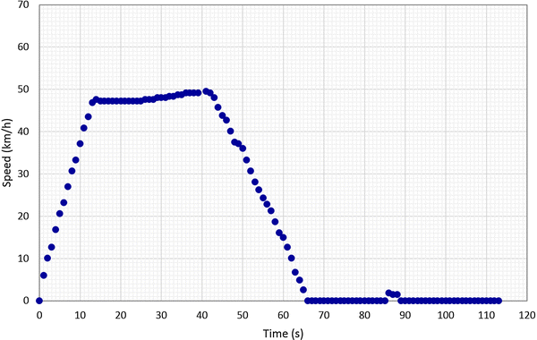
Spurious speed signal example

4.1.3 Discussion
The findings suggest that this initial algorithm is able to extract and classify individual journeys much more quickly than manual processing of the dataset, although a (relatively) brief manual check of the profiles chosen for use in further investigations is still required to correct or discard those where there is any doubt about the classification accuracy. For some applications, this may provide sufficient journeys for use in further investigations. Given the size of the dataset however, manually checking and correcting the entire dataset appeared to be impractical. The algorithm is therefore not suitable if there is a requirement for a large number of journeys with a high level of confidence in the classification accuracy, especially if a representative group of journeys is needed rather than a sample that is biased towards those journeys that are more likely to be classified correctly and are easy to verify.
4.2 Filtering Extraction/Classification Algorithm
4.2.1 Method
The basis of the second algorithm developed was to define additional rules to automatically correct for problems observed during the development of the initial extraction/classification algorithm. This was intended to reduce the amount of manual checking and processing required and hence provide more journey profiles for further analysis.
The initial extraction algorithm was modified in an attempt to filter out the spurious speed signals described above, with four criteria for the start of a new segment:
-
The speed in the previous row is equal to zero (as before).
-
The speed in the current row is greater than zero (as before).
-
The speed X rows ahead of the current row is greater than a threshold Y.
-
The speed in all of the rows between the current row and the current row + X (inclusive) does not equal zero.
The values of X and Y were set to 5 rows and 5 km/h, respectively, based on the duration and maximum speeds of the spurious profiles found while examining the results from the initial extraction/classification algorithm (such as the profile illustrated in Fig. 1). This revised extraction algorithm generated a total of 105,615 individual segments for classification.
Figure 2 illustrates pseudocode for the filtering extraction algorithm. Comment lines (% …) summarise the function of larger blocks of code. Column 5 of the ‘raw_data’ array contains speed.

Pseudocode for the filtering extraction algorithm
Pseudocode for the initial extraction algorithm can be obtained by removing the third and fourth condition from the first IF statement. The initial classification algorithm was also modified with an additional stage to recognise in-segment stops. If two ‘(unknown)’ segments were found between two already classified segments that have only one segment identity between them in the reference database, and the combined distance of the two ‘(unknown)’ segments was within the distance threshold of this missing reference segment identity, the identity of the first of the two segments was set to the identity of the missing segment and the identity of the second was set to ‘(in-segment stop)’. The index file was then modified in accordance with Table 2, so that the first segment reflects the complete journey segment, with the in-segment stop considered as part of the movement time. The second segment then records only the time and duration of the in-segment stop.
Figure 3 illustrates pseudocode for the filtering classification algorithm. The ‘station_distances’ database contains all possible segment identities and the corresponding station-to-station distances, ordered as a continuous journey that visits every station in the network in each direction (repeating sections of the network if necessary). Column 6 of the ‘journey_segment’ array contains distance.

Pseudocode for the filtering classification algorithm
Pseudocode for the initial classification algorithm can be obtained by removing the third FOR loop
4.2.2 Results
This revised classification algorithm identified a total of 98,691 segments from the set of 105,615 (around 93%), a significant improvement on the 82% of the initial extraction/classification algorithm. These improvements meant that it became practical to manually examine the entire dataset and make corrections where the index showed problems, which were typically manifested as unexpected ‘(unknown)’ segments, or single journey segments being assigned a specific identity despite the train almost certainly moving to/from/within the depot or sidings at the time. In total, 638 corrections were required, which changed 2609 of the 105,615 segment identities. 97.5% of the segment identities assigned by the algorithm remained unchanged. This resulted in a slight increase in the number of segments with a specific identity to 99,404.
To make this manual correction process possible in a reasonable time, a number of VBA macros were written for the Excel index file to display the speed profile for individual segments, flag segments with unusually high or low energy consumption and automate the process of recording and implementing corrections. The following bullet points summarise the issues that were most often encountered:
-
There were some cases with more than one in-segment stop, typically on sections of the route where stations are spaced further apart and signals are closer together. The same principles were applied as for the single in-segment stop outlined above, with the first of the unknown segments in the index being modified to reflect the complete station-to-station journey, and the other unknown segments recording only the time and duration of the stops.
-
A similar issue was encountered when there were one or more in-segment stops in consecutive station-to-station journeys, resulting in larger gaps between segments with identities already assigned by the algorithm. The groups of segments for each specific station-to-station journey within the unknown set were treated in the same way as above to fill these gaps.
-
During the autumn season with falling leaves, there were some days with a large number of what appeared to be wheel slide events, with the speed dropping rapidly to zero for a few seconds during braking, before returning to a value consistent with the overall deceleration profile. This meant that distances were being incorrectly calculated, as highlighted by Sect. 3.1. Furthermore, this also created additional spurious in-segment stops, preventing the algorithm from classifying the segments.
-
A specific issue arose where a set of consecutive stations had very similar station-to-station distances, with the last of these immediately followed by a longer station-to-station segment that included a lineside signal at a similar distance to the station-to-station distance shared by the preceding set. As a result, if a train stopped at this signal, the best matching group of reference distances found by the algorithm was for the train to reverse within the set, preventing the following segment from being identified correctly.
-
There were typically gaps in the data on some nights (and a few days) for scheduled maintenance that required the train to be isolated from the power supply. There were a small number of other gaps in the data however, lasting from a few hours to around a day. These may have been due to a fault with the train that resulted in the traction supply being isolated, or a fault with the data collection equipment itself.
There were 16 occurrences of another problem that initially appeared to be a measurement error, with a series of segments displaying very low energy consumption, typically lasting a few minutes to an hour. The train speed profile did not appear to be exceptional, but the line current remained low for the duration of the segment, at a level consistent with only feeding the auxiliaries. Drops in the line voltage consistent with traction current being drawn were observed however, which suggests that the traction equipment had been isolated on the vehicle with the measuring equipment, with other vehicles in the train providing all of the tractive effort. Closer inspection of the speed profile also suggested that the train was running with reduced tractive effort: Figure 4 illustrates two speed profiles for the same station-to-station segment, measured a few hours apart on the same day, with the reduced traction case referring to a segment with very low energy consumption. This also raises the possibility that there may also be a small number of cases within the dataset where other vehicles in the train have their traction equipment isolated, and the vehicle with the measurement equipment is providing a greater share of the total tractive effort. This situation would likely affect the relationship between journey times and energy consumption, but is more difficult to detect in the algorithm results.

Comparison of speed profiles for normal operation and reduced tractive effort
Another example of a rare problem that is potentially difficult to detect is illustrated in Fig. 5. Two separate instances of wheel slide can be seen, and the timing/duration of the second wheel slide event (at 62 s) was such that the next five data points met all four criteria for the start of a new segment. The algorithm therefore incorrectly assigned the start time of the next segment to be here, rather than at the end of the station dwell time, but the effect on the distances was small and it was still able to correctly classify the segments.

Wheel slide event circumventing segment extraction algorithm
4.2.3 Discussion
The results of the filtering algorithm show that it is possible to write additional algorithm rules to reduce the subsequent manual processing effort required. It would certainly be possible to continue to develop this algorithm, with each iteration including new rules to automate the manual corrections found necessary for the previous iteration. As the number of rules increases, there are fewer and fewer exceptions that require manual processing and corrections, but the rules to handle these exceptions generally become more complex. The results also demonstrated that with every new rule there is a small (but not negligible) risk of unintended consequences. Furthermore, they also highlight that some errors in the results can be much more difficult to find than others. Even though the instances of unintended consequences and hidden errors appeared to be very rare (affecting around 0.1% of the segments), their presence does reduce confidence in the accuracy of the results.
4.3 Heuristic Classification Algorithm
4.3.1 Method
One way to increase confidence in the accuracy of the classification process is to develop and run several different algorithms independently and compare their output. The third classification algorithm developed was a heuristic algorithm, intentionally chosen to provide a contrast with the explicit rule-based algorithms developed earlier. The initial extraction algorithm was reused, and a genetic algorithm implemented for classification. Although it was shown above that the initial extraction algorithm creates additional spurious journey segments compared to the filtering extraction algorithm, it should always be possible to combine these to obtain the correct segments. By contrast, the filtering algorithm was shown to (very occasionally) create segments that did not match with the actual journeys, some of which could be difficult to find and correct in the results.
The performance of a genetic algorithm for a given application is strongly influenced by the way in which the problem is represented, the operators that generate possible solutions and the way that the fitness is evaluated for these solutions. A simple representation for the classification problem at hand is to have one gene for each journey segment, with the set of possible alleles for each gene corresponding to all the possible station-station journey pairs (along with alleles for unknown segments and in-segment stops). However, this is a rather simplistic representation. The solution range would be very large, as it would consist of every possible combination of segment identities. Furthermore, the vast majority of these solutions would be infeasible, as there is no guarantee that the final station of one segment would match the initial station in the following segment.
A second representation was therefore considered, with a small set of alleles that represent instructions rather than segment identities, for example: ‘continue to next station’, ‘reverse direction and return to previous station’, ‘in-segment stop’, ‘move to depot’, and others. A post-processor then runs through these instructions to generate the segment identities. This gives a much smaller range of solution, in which all solutions are feasible. The fitness of potential solutions was assessed by comparing the actual distance travelled in each segment against the reference distance for the segment identity assigned, with a high fitness value for close matches between these distances. The problem with this approach is that the identity assigned to each segment depends on all of the instructions relating to previous segments. For example, changing the first gene from ‘continue to next station’ to ‘reverse direction and return to previous station’ would change every single segment identity and likely completely change the fitness value, whereas making this change in the last gene would only change one segment identity and the effect on the fitness value would be small. This makes it very difficult for the genetic algorithm to converge on better solutions. It is preferable for the fitness of solutions to change smoothly as they evolve, with improvements in fitness tied directly to particular sections of the chromosome, rather than relying on a very specific sequence of mutations to occasionally create a large improvement in fitness.
The third representation therefore returned to each gene representing a segment identity, but cut down the number of possible alleles per gene to reduce the number of potential combinations. It also used the fitness evaluation to discourage infeasible solutions. The possible alleles for each gene were found by a pre-processor that compared the distance travelled in the respective segment against the list of reference distances and only allowed segment identities that were within a given threshold (set to 10%, as with the initial classification algorithm). The fitness evaluation combined two separate calculations: the difference between the actual distance travelled within a segment and the reference distance (as before), and also the distance between the final station of the previous segment identity and the initial station of the current segment identity. The smaller this distance, the higher the value from this part of the fitness calculation. A distance of zero represents a feasible solution, as the two stations match. The representation and fitness evaluation were implemented in the genetic algorithm, with rank-based tournament selection for both crossover and replacement of population members. The next section details the subsequent tuning of the parameters of this algorithm and the application to an example day from the results of the filtering algorithm.
4.3.2 Results
A series of runs of the algorithm were carried out with different parameters for mutation rate, tournament selection probability, number of crossover points, population size and tournament size. Some example results are illustrated in Fig. 6, showing significant variation in the rate of convergence and final fitness value with different combinations of parameters.

Genetic algorithm tuning
The patterns observed during these trial runs were used to define the improved algorithm. Lower mutation rates tended to converge faster, but to a lower fitness value. Therefore, an adaptive mutation rate (proportional to the number of generations since the last improvement in global maximum fitness) was implemented. Furthermore, the fitness of each individual gene is effectively calculated during the calculation of the overall fitness of each potential solution, and so the mutation rate of each gene was set to be inversely proportional to its fitness. Tournament sizes and selection pressure were also modified to encourage the algorithm to converge more quickly to higher fitness values. Once the amount of time taken per generation was accounted for, there was no discernible difference between larger or smaller population sizes.
These results were also compared to a couple of days from the filtering algorithm results, which had first been subject to additional manual scrutiny. For days where the train only ran during peak hours (which translated to around 150 genes in the chromosome), the improved algorithm was consistently able to reach 80–90% agreement with the manually checked results from the filtering algorithm and required little additional manual work to remove implausible results. However, where the train was in service all day (over 500 genes per chromosome), it was necessary to run the algorithm several times and use a post-processor to select the most commonly occurring alleles in each gene from the set of results in order to reach this 80–90% agreement. This increased the time required to process each day of the dataset to anywhere between a couple of hours to a day or two. By contrast, the initial and filtering algorithms processed each day of the dataset in seconds, many orders of magnitude were faster. Although further development of the genetic algorithm would increase performance, it is unlikely to reduce the running times by the several orders of magnitude required to be competitive with the explicitly designed rule-based algorithms when working on large datasets. As such, further development of heuristic algorithms was not considered promising.
4.3.3 Discussion
The genetic algorithm was able to classify most of the segments relatively quickly from a simple representation and fitness evaluation, but was not able to complete the classification in a reasonable time. Nevertheless, in small-scale tests it did tend to converge towards the results of the filtering algorithm, and so partially achieved the aim of increasing confidence in the results of other algorithms by independently approaching the same results. While further tuning and running different populations in parallel are possible for the genetic algorithm to process large datasets, it is unlikely to address the main problem of very long running time compared to other algorithms.
4.4 Sequence-Based Classification Algorithm
4.4.1 Method
The final algorithm uses the work done during development of the heuristic classification algorithm to reduce the number of possible alleles, with the premise that it may be possible to perform a complete evaluation of all possible combinations of these alleles if the number of options for the identity of each segment is sufficiently reduced.
As with the heuristic classification algorithm, the initial extraction algorithm was used to provide the set of segments. The next step was also the same: a pre-processor to filter out segment identities where the difference between the reference and measured distance was not within a threshold. This pre-processor was then extended to examine the cumulative measured distance of the current and following segments, to generate lists of plausible identities for the current segment if it featured zero, one, two or more in-segment stops.
The next step was to construct plausible sequences of consecutive segment identities, filtering out the identities where the starting station did not match the final station of the previous segment. The following (purely illustrative) example describes this process, using a set of three consecutive segments of 1358, 769 and 1538 m to represent measured data. The six stations in the network are illustrated in Fig. 7.

Example network to illustrate sequence-based classification algorithm
Table 3 illustrates the possible options for the identity of each example segment. A range of ±5% was used to calculate the minimum and maximum thresholds from the measured distances of each segment. The possible station-to-station identities in each case are then the identities of segments whose length (from Fig. 7) lies between the minimum and maximum threshold calculated.
The next step is for the algorithm to try to construct viable sequences of consecutive station-to-station identities. The principle is illustrated in Fig. 8 in tree form. The three columns correspond to the possible station-to-station identities from Table 3. Each arrow represents the algorithm testing whether the final station of the initial segment matches the first station of the following segment. It can be seen from both Table 3 and Fig. 7 that there are several sets of two consecutive station-to-station identities, but only one complete set of three consecutive identities: ED-DC-CB.

Example sequence-based classification algorithm tree
Rather than testing all of the possible permutations (effectively exploring the entire tree), the algorithm was designed to only explore each branch until none of the identities at that level follow nor proceed from the previous one. This is indicated by the different arrow styles/colours in Fig. 8. A solid green arrow indicates a successful test, and a dashed red arrow indicates an unsuccessful test. A dotted grey arrow indicates that testing is not required, as these branches of the tree have already been ruled out by the failure of a previous test. In this simple case, the number of tests that the algorithm must carry out is reduced from 24 to 12. As the number of segments increases, the benefit of this selective approach increases exponentially, and it is in fact required for the algorithm to run in a reasonable time for the case study dataset. For comparison, a total of 1,872 tests would be required for this simple example if the initial filtering against the minimum and maximum distance thresholds was not carried out.
The key question for this method is to determine at what point to terminate the sequences and stop filtering out possible segment identities. Longer sequences will be more likely to positively identify a given segment by filtering out all but one of the initially identified options, but there is an increased risk of an unusual events (such as an ECS movement to/from the depot, or several in-segment stops) interrupting the sequence and leading to all of the options being filtered out and discarded. For the case study in this paper, it was found sufficient to terminate the sequences at segments where the initial pre-processor did not find any possible matches in the reference database, as these segments typically corresponded to an ECS move.
4.4.2 Results
As mentioned previously, the number of corrections required to the data from the initial extraction algorithm meant that the time required for manual processing of the complete dataset would be extensive, and so only the first 3 months of the dataset were examined.
The chosen termination criterion was found to give reasonable results when the reference list of identities only included segments with no in-segment stops, typically exploring all options for the segments within a given day in 1–3 s, and returning identities for 77% of these segments (compared to around 82% for the initial classification algorithm working on this set). Adding the possibility of a single in-segment stop usually took a similar time and returned identities for 72% of the segments, but on a couple of days took several minutes. When the reference lists included two or more in-segment stops the algorithm typically failed to find viable sequences and returned few segment identities, and a different termination criterion would likely be necessary. However, the lists of possible identities found with zero or one in-segment stop proved sufficient.
The sequence-based algorithm found a single identity for around 87% of the segments by combining the lists of identities found for zero in-segment stops and for one in-segment stop. For a further 6% of the segments, the algorithm found several different plausible options, which included the one subsequently chosen during the manual checking process. One of the most common locations for this in the case study dataset was a route section approaching a terminus, where the station-to-station distances between four consecutive stations were all close to 1.3 km. Therefore, as well as the expected A-B-C-D-C-B-A journey, the algorithm also found journeys such as A-B-C-B-C-B-A to be plausible from the sequences of measured station-to-station distances. A second example was segments adjacent to an ECS move to/from the depot, as the depot is located at a junction in the network and there are several route options with similar distances, especially where trains may reverse direction immediately after the ECS move.
For the remaining 7% of the segments that required identities to be chosen manually, the algorithm typically did not find any plausible options. These were typically located in the final service of the day, when the subsequent ECS move to the depot interrupted the sequence and resulted in all the options being discarded. As discussed above, different sequence termination criteria could increase the percentage of segment identities assigned by the algorithm. There were very few examples of misidentified segments: less than 0.2% of the total.
The manually corrected segments generated by the sequence-based classification algorithm were subsequently compared against the results of the filtering algorithm, and 99.8% of the segment identities and index file data (start time, duration and so forth) were in agreement. The close match between the two sets, derived in different ways, suggests that the results of the extraction and classification process are likely to be accurate.
4.4.3 Discussion
The sequence-based algorithm generally identified a lower proportion of the segments than the filtering algorithm. However, an advantage was the much-reduced instances of misclassified segments: the subsequent manual corrections almost entirely consisted of either choosing from a list of plausible options or replacing ‘(unknown)’ segments.
Further development of the sequence termination criteria could improve the proportion of segments that are identified by the algorithm. Additional criteria could also be used to filter out implausible options prior to the construction of sequences to improve performance further. For example, the maximum line speed of reference segments could be compared against the maximum reached during the segment, or individual line speed limits compared against the train speed at given locations within the segment. The sequence termination and additional filtering required will both depend on the characteristics of the dataset in question.
5 Summary of Algorithm Results
5.1 Accuracy
The manual corrections made to the index file can be used to estimate the proportion of the segments in the results that were correctly extracted and classified by each of the algorithms, as shown in Table 4. The accuracy for the raw results of the initial algorithm was estimated by comparing its output with the 3 months of the sequence-based algorithm that was checked manually; around 93% of the segment identities matched. The comparison with the sequence-based algorithm refers to running both the initial/filtering algorithm and the sequence-based algorithm independently and manually checking both sets of results alongside each other.
The errors in the results manifest in different ways. The least damaging is where a segment is mistakenly given the ‘(unknown)’ identity, as this is usually easy to see when surrounded by correctly identified segments. Furthermore, if the results are used in subsequent investigations, the only consequence is a slightly smaller sample size. The consequences for further investigations can be more severe if a segment is given the wrong identity, but this is usually still fairly easy to detect among correctly identified segments. Errors become more serious when they are harder to find, such as where a segment has been misconstructed (the wheelslip illustrated in Fig. 5 for example), or where there is a traction fault with a non-metered vehicle in the train.
5.2 Running Time
Table 5 provides a rough indication of the development and running times for the algorithms developed, together with the time required for manual checking and processing of the results (times are estimated to cover the complete dataset where necessary). The relative importance of the development time to the running/checking times will depend on the overall goal of a given project. If the algorithms are being developed to analyse a single existing dataset, then the development time is important as it is likely to form a significant proportion of the project as a whole. If the algorithms are being developed to use for the analysis of multiple existing and future datasets, then it is worth spending more time on development if it results in significant reductions in running/checking times.
In this case, the reduced development time of the heuristic algorithm compared to other rule-based algorithms did not compensate for the long runtimes required to achieve similar accuracy. Heuristic algorithms are typically better at solving problems where there may be little information from which to create explicit rules, and where a better (rather than perfect) solution is desired. For the classification problem in this paper, there is a reasonable amount of information available, which allowed the specific rule-based algorithms to be designed. As such, the chief purpose of the heuristic algorithm was an additional check to increase confidence in the results of other algorithms rather than to classify the entire database.
Comparison of the filtering algorithm with the initial algorithm results illustrates the trade-off between the extra time required to develop dataset-specific rules and the reduction in time required for manual checking and processing of the exceptions. The time required for these corrections very much depends on the size and features of the dataset in question. In this case, removing the spurious speed signals illustrated in Fig. 1 was the most important part of the filtering algorithm that made manual checking of the complete dataset possible. As discussed above, there is a small chance of unintended consequences with each additional rule introduced however.
The difference between the running times of the initial/filtering and sequence-based algorithms was small enough (minutes) to be negligible for the single dataset in this experiment. Nevertheless, it is worth noting that the time taken to run the sequence-based algorithm was still a multiple of the initial/filtering algorithms. Furthermore, without suitable filtering and termination criteria, operation times of the sequence-based algorithm can easily change from seconds to hours, or even days.
6 Conclusions
The increase in the amount of information being gathered about technological systems such as railways provides significant potential to improve their design and operation. Processing and analysing large datasets manually to extract useful information becomes impractical however, requiring the design of algorithms to analyse data and maximise the usefulness of the datasets. Without manual oversight of the complete dataset, a key issue when building algorithms for this purpose is their accuracy.
This paper considered the design of algorithms to extract and classify individual station-to-station segments within a large speed profile dataset. The development work highlighted that it becomes increasingly difficult to construct a perfect ‘black box’ algorithm to correctly classify all of the possible situations and unusual/exceptional events in a given dataset. As the algorithms are refined further, the development time and algorithm complexity are likely to increase significantly for smaller and smaller increases in accuracy. There is a balance to be struck between the accuracy required, the algorithm development time, the algorithm running time and the time required for further manual checking/processing of the results.
The results obtained in this paper in a case study of a metro system suggest that the most promising approach for this problem is to check the cumulative distance of several consecutive journey segments against a set of reference station-to-station distances, along with additional dataset-specific rules defined for pre-processing and post-processing of the data. This filtering algorithm was able to reach a good level of accuracy in a shorter overall time than other algorithms. If greater confidence in the accuracy of the results is required, then checking the results of the filtering algorithm against a second sequence-based algorithm appears to be the best strategy. The sequence-based algorithm builds up plausible sequences of individual journey segments and is a good fit for validation of other algorithms, as it has a lower likelihood of assigning incorrect identities and illustrates all possible options rather than only the best match. However, the sequence-based algorithm is less resilient to unusual events and imperfections in the input data—these events typically resulted in all of possible options being discarded and no identities returned. This lack of resilience in the sequence-based algorithm is a key reason why the filtering algorithm described above was preferred. A heuristic (genetic) algorithm was also examined, but for this application there is enough specific information about the dataset for algorithms based on explicit rules to be constructed, and these were orders of magnitude faster than the heuristic algorithm.
In their current form, the algorithms developed in this paper could be directly applied to data from other railway systems. However, it has been highlighted that the performance of the algorithms depends on the characteristics of the railway system in question. For example, the frequency of station stops could significantly affect the algorithm performance and suitability. Two major areas for further work are therefore to examine this performance using datasets from other railway systems and also to develop and compare the performance of algorithms based on other characteristics, such as speed limits rather than station stops. Further development work for the algorithms already developed could include hybridisation of the filtering and sequence-based algorithms, along with the index file macros, to further automate the process and reduce the amount of manual work required. Finally, the work described in this paper has provided an extensive dataset of energy consumption and train running data, and further projects are already underway using this dataset to investigate in detail how operational performance and energy efficiency can be improved in urban rail systems.
Change history
30 January 2019
The first sentence of Abstract should be “The rapid increases in the quantity of data being gathered from technological systems such as railways can be used to improve their design and operation”.
References
Longo G, Medeossi G, Nash A (2012) Estimating train motion using detailed sensor data. In: Transportation research board 91st annual meeting, Washington D.C., USA, 22nd–26th January 2012
Pritchard J, Preston J, Armstrong J (2015) Making meaningful comparisons between road and rail—substituting average energy consumption data for rail with empirical analysis. Transp Plan Technol 38(1):111–130. https://doi.org/10.1080/03081060.2014.976985
Geistler A (2002) Train location with eddy current sensors. In: Allan J, Hill RJ, Brebbia CA, Scuitto G, Sone S (eds) Computers in railways VIII. WIT Press, Ashurst, pp 1053–1062. https://doi.org/10.2495/cr021041
Heirich O, Lehner A, Robertson P, Strang T (2011) Measurement and analysis of train motion and railway track characteristics with inertial sensors. In: 2011 14th international IEEE conference on intelligent transportation systems (ITSC), 5–7 Oct 2011, pp 1995–2000. https://doi.org/10.1109/itsc.2011.6082908
Powell JP, Palacín R (2015) Passenger stability within moving railway vehicles: limits on maximum longitudinal acceleration. Urban Rail Transit 1(2):95–103
Allotta B, Colla V, Malvezzi M (2002) Train position and speed estimation using wheel velocity measurements. Proc Inst Mech Eng Part F J Rail Rapid Transit 216(3):207–225. https://doi.org/10.1243/095440902760213639
Malvezzi M, Vettori G, Allotta B, Pugi L, Ridolfi A, Rindi A (2014) A localization algorithm for railway vehicles based on sensor fusion between tachometers and inertial measurement units. Proc Inst Mech Eng Part F J Rail Rapid Transit 228(4):431–448. https://doi.org/10.1177/0954409713481769
Ernest P, Mazl R, Preucil L (2004) Train locator using inertial sensors and odometer. In: IEEE intelligent vehicles symposium, 2004, 14–17 June 2004, pp 860–865. https://doi.org/10.1109/ivs.2004.1336497
Druet E, Bilenne O, Massar M, Meers F, Lefèvre F (2006) Interval-based state estimation for safe train positioning. In: 7th world congress on railway research, Montreal, Canada, 4th–8th June 2006
De Fabris S, Longo G, Medeossi G (2010) Automated analysis of train event recorder data to improve micro-simulation models. In: Hansen IA (ed) Timetable planning and information quality. WIT Press, Ashurst, pp 125–134
Powell JP, Palacin R (2016) Stile di guida con ERTMS livello 2 e segnalamento convenzionale lungo linea: uno studio esplorativo [Driving style for ERTMS in-cab and conventional line side signalling: an exploratory study]. Ingegneria Ferroviaria 71(12):927–942
Acknowledgements
The authors would like to thank the metro system operators that made data available for this research, and Mr. Sam Johnson (undergraduate mechanical engineering student) for additional work in MATLAB.
Open Access
This article is distributed under the terms of the Creative Commons Attribution 4.0 International License (http://creativecommons.org/licenses/by/4.0/), which permits unrestricted use, distribution, and reproduction in any medium, provided you give appropriate credit to the original author(s) and the source, provide a link to the Creative Commons license, and indicate if changes were made.
Author information
Authors and Affiliations
Corresponding author
Additional information
Editor: Xuesong Zhou.
Rights and permissions
Open Access This article is licensed under a Creative Commons Attribution 4.0 International License, which permits use, sharing, adaptation, distribution and reproduction in any medium or format, as long as you give appropriate credit to the original author(s) and the source, provide a link to the Creative Commons licence, and indicate if changes were made.
The images or other third party material in this article are included in the article’s Creative Commons licence, unless indicated otherwise in a credit line to the material. If material is not included in the article’s Creative Commons licence and your intended use is not permitted by statutory regulation or exceeds the permitted use, you will need to obtain permission directly from the copyright holder.
To view a copy of this licence, visit https://creativecommons.org/licenses/by/4.0/.
About this article

Cite this article
Powell, J.P., Palacín, R. Development and Comparison of Algorithms to Derive Vehicle Location from Speed Profile Data. Urban Rail Transit 5, 48–63 (2019). https://doi.org/10.1007/s40864-018-0077-5
Received:
Revised:
Accepted:
Published:
Issue Date:
DOI: https://doi.org/10.1007/s40864-018-0077-5