
Abstract
Positron emission tomography (PET) is a highly quantitative imaging modality that can probe a number of functional and biological processes, depending on the radio-labelled tracer used. Static imaging, followed by analysis using semi-quantitative indices, such as the standardised uptake value, is used in the majority of clinical assessments in which PET has a role. However, considerably more information can be extracted from dynamic image acquisition protocols, followed by application of appropriate image reconstruction and tracer kinetic modelling techniques, but the latter approaches have mainly been restricted to drug development and clinical research applications due to their complexity in terms of both protocol design and parameter estimation methodology. To make dynamic imaging more feasible and valuable in routine clinical imaging, novel research outcomes are needed. Research areas include non-invasive input function extraction, protocol design for whole-body imaging application, and kinetic parameter estimation methods using spatiotemporal (4D) image reconstruction algorithms. Furthermore, with the advent of sequential and simultaneous PET/magnetic resonance (MR) data acquisition, strategies for obtaining synergistic benefits in kinetic modelling are emerging and potentially enhancing the role and clinical importance of PET/MR imaging. In this article, we review and discuss various advances in kinetic modelling both from a protocol design and a methodological development perspective. Moreover, we discuss future trends and potential outcomes, which could facilitate more routine use of tracer kinetic modelling techniques in clinical practice.
Introduction
Positron emission tomography (PET) is a powerful and highly specialised imaging modality for the non-invasive measurement of different physiological and biological processes at a molecular level. Although the emission tomography theory also applies to PET, the data acquisition in PET differs significantly from the data acquisition in the well-known single-photon emission computed tomography technique. The principles of PET are based on the fact that by labelling a compound with a positron-emitting isotope and intravenously injecting it into a patient in tracer quantities, one can detect its bio-distribution inside the body and investigate a number of physiological and biochemical processes such as perfusion, proliferation and glucose metabolism.
During the last few years, a number of studies have highlighted the potential diagnostic role of kinetic modelling, which is able to provide additional parameters, more closely related to the underlying pathology. At the same time, kinetic analysis can assist in drug development and therapy response monitoring through drug labelling and subsequent kinetic parameter evaluation.
The potential benefit of kinetic analysis has been demonstrated for a number of tracers and in a number of different pathological conditions. In head and neck imaging and specifically in central nervous system lymphomas, kinetic analysis of dynamic 18-F-labelled 2 deoxy-2-d-glucose (18F-FDG) may help in diagnosis as well as response monitoring (Fig. 1) [1, 2], providing more reliable tumour detection estimates [3]. Using 18F-DOPA, Schiepers et al. [4] demonstrated the importance of kinetic modelling in tumour-grade differentiation, while Thorwarth et al. [5], using 18F-FMISO, showed a high correlation between kinetic parameters and response to therapy. Similar findings were reported using 18F-FLT in brain tumours by Schiepers et al. [6], who showed a correlation between kinetic parameter estimates and disease progression, while Wardak et al. [7], in their study in glioma patients, highlighted the significance of full kinetic modelling in therapy response monitoring. In lung cancer, dynamic 18F-FDG imaging followed by kinetic analysis has been shown to assist in differentiation between squamous cell carcinoma and adenocarcinoma, revealing differences in kinetics between these subtypes [8]. In colorectal tumours, kinetic analysis may help to differentiate between primary tumours and normal tissue [9], and kinetic parameters may provide information on proliferation and angiogenesis [10, 11]. The literature contains a multitude of studies highlighting the potential significance of kinetic modelling in clinical oncology and drug development, as several critical reviews have shown [12–14].

MR and FDG PET images in a 47-year-old male patient with diffuse large B cell CNS lymphoma. Contrast T1-weighted MR image shows multiple enhancing lesions in the bilateral paraventricular area (a). Baseline dynamic FDG PET shows an increase in K 1 , k 3 and CMRGlc and a decrease in k 2 at lymphoma lesions (b). Follow-up dynamic FDG PET shows a decrease in all four parameters (c). Reprinted with permission from [170] (color figure online)
The following discussion focusses mainly but not exclusively on clinical 18F-FDG PET imaging, given that 18F-FDG is the most commonly used tracer. First, we briefly discuss some aspects of kinetic modelling and its role in oncology. We elaborate on the pitfalls of static imaging, the clinical importance of dynamic imaging and tracer kinetic analysis, and the difficulties associated with its adoption in clinical practice. We then review established but most importantly new strategies for tracer kinetic analysis, focussing particularly on input function (IF) extraction, whole-body parametric imaging, kinetic parameter estimation and simultaneous dynamic PET and magnetic resonance (MR) data acquisition. Finally, we discuss future perspectives based on current and emerging advances in software and hardware.
PET imaging in oncology
Positron emission tomography (PET) is a well-established imaging modality in oncology, having been used in the past two decades for numerous studies, involving many benign and malignant abnormalities. One of the radiopharmaceuticals most frequently used is 18F-FDG [15, 16]. As FDG (a glucose analogue) and glucose are similar, they compete during phosphorylation. The two byproducts, FDG-6-phosphate and glucose-6-phosphate, follow different routes. Glucose is further metabolised into fructose-6-phosphate, while FDG is trapped. Increased expression of glucose transporters and enzymes responsible for metabolism can contribute to this glucose accumulation and consumption. FDG uptake is also regulated by the hypoxic nature of the tumour as well as by cellular proliferation and impaired tumour-suppressing mechanisms [17].
The two-tissue compartmental model can adequately describe the kinetics of FDG. Two differential equations can describe the concentration change rate in each compartment to analytically derive the operational equation.
The first compartment is the free tracer and the second one is the trapped FDG-6-phosphate. The tracer enters the free pool with a rate constant equal to K 1. In the free pool, the tracer can either be cleared with a rate k 2 and a fractional clearance rate K 1 k 2 /(k 2 + k 3), or become trapped with a rate k 3 and a fractional uptake rate K 1 k 3 /(k 2 + k 3) = K i .
After using Laplace transformations, the aforementioned compartmental concentrations can be written as
And the overall sampled PET signal as
where
C b is the arterial whole blood tracer concentration, and Va is the fractional blood volume. For dynamic scans not exceeding 60 min, it makes less sense to exclude a k 4 constant rate as it becomes difficult to obtain reliable estimates. However, while including this parameter may improve the model fit, in certain regions, such as the liver, an assumption of k 4 = 0 is not completely valid. Furthermore, the absence of a k 4 may lead to reduced estimates of the metabolic rate of glucose (MRGlu) [18].
Pitfalls in static clinical 18F-FDG imaging: why dynamic imaging?
PET scanners are highly specialised cameras that, in principle, work in a similar way to normal digital cameras, by collecting photons over a period of time, to produce a static image from the integrated measurements. This mode of imaging is almost exclusively used in clinical practice, for qualitative assessment and visual inspection and interpretation of the reconstructed images. However, quantitative estimates related to the accumulation of a radio-labelled compound have complemented or superseded visual interpretation in many clinical applications and provide a more objective assessment of the system under study.
Semi-quantitative indices such as the standardised uptake value (SUV) can provide valuable information regarding the system under study and can help in interpretation, differentiation and analysis of clinical scans for tumour detection, staging and response monitoring.
SUV is a simplified metric that requires single temporal-frame imaging:
It is frequently used in oncology as a simple method of basic quantification in static imaging protocols and it provides a surrogate estimate of biologically related parameters. The SUV can actually be viewed as an estimate of the kinetic influx rate K i , and the accuracy in the estimation depends on the following two conditions:
-
(a)
in the voxel or region of interest (ROI), the contribution of non-phosphorylated FDG (which includes the vascular and the extravascular compartments) must be negligible relative to phosphorylated FDG (a commonly used two-tissue compartmental model is shown in Fig. 2).
Fig. 2 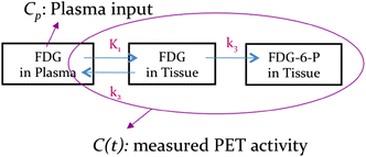
The two-tissue compartmental model. The interstitial space and cellular space are commonly lumped together as the first tissue compartment. K 1 and k 2 are associated with the tracer influx and venous clearance of FDG in and out of this compartment, and k 3 captures the intracellular phosphorylation rate. The measured PET signal C(t) cannot distinguish between non-phosphorylated and phosphorylated compartments. For dynamic scans of <60 min and in most organs a three constant rate model is more appropriate (color figure online)
-
(b)
the time integral of plasma FDG concentration is proportional to the injected dose divided by body weight (BW), lean body mass (LBM) or body surface area (BSA) as used in the SUV metric (the latter two are somewhat more reliable and less prone to artificial increases or decreases due to changes in body habitus, of the kind that commonly occur, for example, among oncology patients undergoing treatments) [19–21].

These two assumptions can however break down in clinical PET imaging and lead to noticeable inaccuracies [22–25]. As regards the first assumption, less FDG-avid tumours that have relatively small FDG phosphorylation rates may not be optimally imaged at standard imaging times (e.g. 60 min after injection) due to contributions of the vascular compartment and/or intracellular non-phosphorylated FDG, thus resulting in limited differentiability between diseased and normal tissue or organs [26]. This can be a particular issue post-therapy when there can be substantial background FDG activity in tissues [27]. This also leads to spatial distributions for SUV images that vary over time.
As regards the second condition, if a patient is for instance undergoing chemo- or hormone therapy, the dynamics of plasma FDG could be significantly affected, and the time integral of the plasma FDG could deviate from what would be predicted from the dose and BW/LBM/BSA alone [24, 28]. The SUV estimate for such a case may thus not accurately correspond to the kinetic influx rate, and the therapy response may not be accurately reflected by the change in SUV. This also explains why patient populations showing varying plasma dynamics result in scattered correlation between the SUV and K i measures [29].
Overall, the single-time-point SUV PET/CT methodology has documented limitations [30–34]), and may underestimate disease presence in certain malignancies [22]. A more advanced approach, namely dual-time-point FDG PET imaging, proposes to measure the retention index as the percent change in SUV images from early (~60 min) to late (90–180 min) scans [35–44].
A solution to the second shortcoming is to supplement the PET scan with blood sampling data, arriving at the fractional uptake rate (FUR) measure [45, 46]. This approach, in its original form, involved invasive blood sampling from the time of injection. A closely related approach, referred to as simplified kinetic analysis (SKA), utilised population-based IFs, and blood samples collected late-phase to scale the population-based IF [47]. In any case, the FUR/SKA approaches, like the SUV framework, continue to fail to correct for the presence of non-phosphorylated FDG and blood volume presence [48].
When dynamic methods are used, micro-parameters (i.e. individual rate constants between compartments) or macro-parameters (i.e. combinations of micro-parameters) have to be estimated using multiple time courses of the activity concentration in the tissue of interest.
The MRGlu can thus be calculated as \( {\text{MRGlu}} = \frac{{C_{\text{b}} }}{LC}\frac{{K_{1} k_{3} }}{{k_{2} + k_{3} }} \) with the lumped constant being the difference in transport and phosphorylation between glucose and FDG and C p the arterial plasma glucose concentration.
In a comparative study, Cheebsumon et al. [49] found that fractional changes in assessing response to therapy were under-estimated using SUV compared to Patlak analysis (Fig. 3), even after correcting for plasma glucose levels.

Relative percentage changes in the standardised uptake value (SUV) and simplified kinetic analysis (SKA) due to therapy compared with corresponding changes in MRGlu-Patlak on a lesion-by-lesion basis for SUVBW (triangles), SUVLBM (circles) and SUVBSA (squares) (a) uncorrected for blood glucose and (b) corrected for blood glucose, and (c) for SKM. All simplified methods showed a substantially smaller fractional change than with Patlak analysis, emphasising the importance of kinetic analysis in assessing response to therapy. Reprinted with permission from [49]
Several other studies have compared a number of semi-quantitative methods based on static protocols (SUV, simplified kinetic method) with kinetic analysis methods based on dynamic imaging protocols (Patlak graphical analysis and full compartmental modelling), further motivating the need for dynamic imaging [50, 51].
Challenges in the clinical adoption of pharmacokinetic modelling
Traditionally, application of dynamic imaging protocols, followed by graphical analysis or full kinetic analysis modelling strategies, has been mainly restricted to clinical research. The limited adoption of dynamic imaging protocols in clinical practice stems from the technical difficulties associated with pharmacokinetic modelling, which make these techniques difficult to adopt in routine clinical practice. We here discuss these difficulties, while “Summary and future perspectives” section elaborates upon advanced strategies to address some or all of these issues.
One of the main issues associated with clinical adoption of kinetic modelling is the need to have an accurate estimate of the tracer’s activity concentration in the blood over the course of the dynamic study. Obtaining an arterial IF through continuous or manual discrete blood sampling is the gold standard; however, it is invasive, time consuming and technically challenging, and requires extensive facilities and specialised personnel.
Another important issue is the limited anatomical field of view (FOV) coverage offered by current PET systems (15–25 cm), which restricts dynamic acquisition protocols to a specific part of the body. Therefore, kinetic modelling strategies have so far been limited to single-bed acquisition protocols, making them ill-suited for whole-body parametric imaging applications. Furthermore, dynamic imaging protocols can last for up to 1.5 h post-injection and therefore impact on patient comfort, as well as patient throughput.
Choosing the correct model is very important and it depends upon the administered tracer, the target region and the scanner characteristics. In most cases, the actual underlying true physiological model is too complicated to identify, due to the statistical variations of the measured data and limitations introduced by the instrumentation. A simplified model is therefore chosen in most cases as a trade-off between statistical reliability of the derived parameters and error due to the use of a simplified model. Furthermore, due to the limited counting statistics, parameter estimation is usually performed at a regional level, following ROI delineation based on anatomical information and kinetic model application. This method is attractive as many voxels are summed together, improving the statistics and resulting in reliable parameters. However, as the underlying tissue contains heterogeneous kinetics, the average that is calculated when estimating regional kinetics inevitably results in biased estimates. In addition, the spatial average limits the spatial information that PET data can potentially provide.
To avoid averaging heterogeneous kinetics and preserve the spatial resolution, one should model the kinetics at the scanner’s finest image discretisation element, which is the voxel. In this way, parametric images are obtained, which allow the spatial heterogeneity of the physiological parameters to be assessed. However, although parametric imaging has benefits compared with regional analysis, it suffers from increased noise due to reduced counting statistics at the voxel level. This results in bias and non-statistically reliable parameter estimates if full kinetic analysis is performed. Also, computational time becomes an important parameter. To address the excess noise while maintaining the spatial information, and to improve the signal-to-noise ratio (SNR), post-reconstruction techniques can be used. These methods are expected to improve kinetic parameter precision and accuracy but parameter estimation is performed using independently reconstructed images, which leads to suboptimal parameter estimation due to limited counting statistics and inaccurate modelling of the noise in the data. Direct 4D parameter estimation methods in which kinetic parameters are directly estimated during image reconstruction provide a promising alternative as they can improve upon kinetic parameter bias and variance. However, until recently, the slow convergence properties of these reconstruction algorithms and their added complexity have prevented their more frequent application. New developments in these areas are discussed in the next section.
Advanced strategies in pharmacokinetic modelling
As mentioned previously, there are a number of challenges associated with the clinical adoption of kinetic modelling strategies in clinical practice. However, during the last few years advances in data analysis, protocol design and instrumentation have provided a solid foundation for more widespread use of dynamic imaging, followed by fully quantitative analysis, in the clinic. In the rest of this article, we review techniques and recent advances in key areas associated with pharmacokinetic modelling and discuss their potential application in routine clinical practice.
Input function estimation
Kinetic imaging requires accurate calculation of the IF. Arterial blood sampling is an invasive and complicated method which makes scanning very uncomfortable for the patient and virtually impossible to translate into clinical practice. Consequently, numerous techniques have been proposed to calculate the IF from images as a convenient and non-invasive alternative to arterial cannulation [52]. However, even image-derived input function (IDIF) estimation is by no means an easy task and there are several issues to be addressed if such a methodology is to be applied in clinical practice. Here, we list a few of them [53].
-
Segmentation of the blood pool: One of the difficult aspects is to locate the ROI through relevant information, e.g. carotid arteries. Many researchers have attempted segmentation of regions using the early time frames of the dynamic PET images. This is very difficult as PET resolution is limited to about 4–5 mm, making the segmentation of small structures a difficult task. A way to solve this issue is to segment the arteries using angiograms acquired from other imaging modalities as shown in Fig. 4 [54]. Fung and Carson, for example, recently proposed a method using high-resolution MR images of the carotid arteries [55]. This technique along with another recent investigation by Iguchi et al. [56] may be seen as promising examples to translate into simultaneous PET/MR imaging, a recently developed field. Such a translation might be more complicated in whole-body imaging compared with brain imaging, due to additional sources of motion. A region that could be used for obtaining the blood pool is the cardiac cavity or ascending aorta, however such IDIF extraction is generally limited to acquisitions that include these structures within the FOV.
Fig. 4 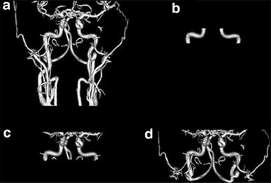
Three-dimensional rendering of segmented artery from time-of-flight magnetic resonance angiography images (a); the arterial region of interest (ROI) version one (b); the arterial ROI version two (c); and the arterial ROI version three (d). Reprinted with permission from [54]
-
Limited spatial resolution: PET imaging has limited spatial resolution due to partial volume and motion effects [57]. In brain imaging, motion is relatively simple to correct by applying frame-by-frame realignment or measuring rigid motion with the use of external devices [58]. As such, the main effect for limiting resolution is partial volume, with activity spilling in and out. Fung and Carson, for example, attempted to minimise this complication by selecting only a centreline [55]. On the other hand, in whole-body imaging, respiratory motion is a major challenge as it can significantly degrade spatial resolution and it is the main limiting factor for quantitative imaging [59]. Motion correction approaches have been proposed using PET/MR imaging but such approaches are still in their early stages [60] and will require further work before they can be translated into clinical PET/MR protocols. However, in the body, since the regions used to extract the IF are relatively large compared to the carotids in the brain, partial volume effects can be less of a concern.
-
Plasma versus whole blood and metabolites: Even if the IF is calculated, there are several cases in which it is necessary to calculate the amount of metabolites in the blood as they augment the background signal without necessarily participating in the kinetics. However, in some cases, metabolites may show competitive kinetics in some organs [61]. Fortunately, in 18F-FDG imaging, no metabolite correction is necessary while the difference between plasma and whole-blood concentration is minimal and the ratio between the two also remains relatively constant over time. However, for a large number of tracers, metabolite correction is necessary and it is very difficult to achieve this using IDIF as it is not possible to distinguish the parent radiotracer from the corresponding radio-metabolites [62]. In a similar context, it is necessary to distinguish the amount of radioactivity in the blood and the plasma because only the latter participates in the biochemical exchanges, while the radiotracer in the blood only augments the PET signal [63]. As an attempt to produce a robust holistic approach to extract IDIF for whole-body tracer kinetics, a novel analysis was recently proposed by Huang and O’Sullivan [64].
-
Limited temporal resolution: PET in theory offers very high temporal resolution (less than a nanosecond) but in practice its spatiotemporal resolution is limited by the need to measure, within a timeframe, enough counts to allow the extraction of quantitative information. In particular, for the calculation of the peak of the IF, a temporal resolution of a couple of seconds is needed. Current iterative reconstruction algorithms are able to provide high spatial resolution images but, within this timeframe, they fail to produce quantitative results due to noise-induced bias generated from the non-negativity constraint [65]. Furthermore, using graphical analysis methods (such as Patlak) where the area under the input curve is important and when using tracers with metabolites mainly at the late frames, the coarse sampling in the early frames, where the activity changes rapidly, will introduce errors in the subsequent kinetic parameters. This is because the approximately estimated area under the peak (AUP) accounts for a significant proportion of the total area under the curve (AUC) following metabolite correction; in comparison, with non-metabolised tracers, the AUP is only a small fraction of the AUC [66].

In particular cases in which some regions in the brain exhibit simple and well-understood biochemical exchanges with the arterial IF, the kinetic parameters of the brain can be expressed in relation to the kinetic behaviour of this reference region [67]. These models are known as reference tissue models and have proven valuable for kinetic analysis of dynamic PET imaging of brain function [68]. However, these models depend upon a suitable reference tissue, which might not be apparent across a large range of patients, and they are limited to particular tracers. Other methods, defined population-based, estimate the IF from a library of IFs [69]. Another family of methods attempts to estimate simultaneously the IF and the kinetic parameters by fitting multiple time-activity curves at the same time [70, 71]. Expanding this direction of research further, Reader et al. [72] jointly estimated the IF and spectral coefficients directly from list-mode data using fully 4D image reconstruction. However, these methods do not necessarily estimate the true IF but an IF that provides the best fit to the data.
Overall, the translation of IF to whole-body parametric imaging is dependent on the tracer, the clinical application and the organ of interest. It will be necessary to reconsider approaches currently in use, such as the IDIF methods, and make them more robust by incorporating the power of new multimodality imaging techniques such as PET/MR, as will be further discussed [73].
Towards dynamic whole-body parametric imaging
Dynamic PET imaging has so far been largely treated (incorrectly) as mutually exclusive with whole-body imaging. However, routine clinical multi-bed PET imaging commonly involves single temporal-frame imaging. Clinically feasible combination of whole-body and dynamic imaging raises the following issues: (1) the presence of temporal gaps for any given bed position, and (2) the need for non-invasive quantification of the IF. The first issue is addressed through graphical Patlak analysis, which can be applied with as little as two time point measurements. Although parametric images of K i using Patlak analysis are routinely used in clinical research and for single-bed dynamic acquisitions, until recently their application to clinical practice for whole-body imaging had not been demonstrated. The second issue, however, is particularly challenging.
A particular study by Ho-Shon et al. [74] proposed optimisation of multi-bed dynamic PET acquisitions, based on a statistical Bayesian regression method. This approach focussed on ROI-based parametric analysis and included demonstration of two-bed acquisition examples with uneven bed frames and bi-directional scanning. Similarly, Hoh et al. [75] proposed a multi-bed dynamic acquisition to allow for ROI-based Patlak analysis over multiple beds. Later, Sundaram et al. [76], motivated by the previously mentioned SKA method, and also picking up on the suggestion by Hoh et al. proposed a short two- or three-bed late dynamic acquisition as a simplified alternative to multi-bed Patlak analysis for ROI-level parametric analysis. Kaneta et al. [77] also conducted multi-bed dynamic acquisition of human subjects (0–90 min post-injection) in the context of imaging hypoxia using 18F-FRP170, involving multi-pass whole-body acquisitions, each lasting for 12 min (6 beds × 2 min/bed). However, only dynamic images were presented, without tracer kinetic modelling.
The Patlak model uses the time integral of the IF [78]. A novel work by van den Hoff et al. [79] proposed a solution beyond this. Utilising whole-body dual time-point image acquisition, and denoting C(t) and C p (t) as the measured PET activity for a given voxel and the IF from the heart, respectively (as seen in Fig. 1), each measured at times t 1 and t 2, the authors showed that the Patlak slope K i is estimated as:
where \( \overline{V} \) denoted a population-based estimate of the Patlak intercept. The results indicated excellent correlation (r = 0.99) with actual Patlak measured slopes, even when the second term in the above equation was dropped (r = 0.98), although in this case, the slope of regression changed substantially from zero. This approach was primarily validated using single-bed imaging (n = 9), but also included application to a single whole-body scan including both the brain and the torso.
Recently, another whole-body PET imaging scheme including optimisation and validation was proposed in companion papers by Karakatsanis et al. [80, 81]. This approach involved a 6-min initial scan over the heart, as well as generation of dynamic whole-body datasets (6 passes), the latter shown in Fig. 5. This enabled a non-invasive solution to IF estimation by combining the first 6-min scan over the heart (capturing the early dynamics) and subsequent passes over the heart. Standard Patlak linear graphical analysis modelling was employed at the voxel level (Eq. 11), coupled with plasma IF estimation from the images, to estimate the tracer uptake rate K i (slope), resulting in parametric images at
the individual voxel level. The images (as seen in Fig. 5) convey a different ‘feel’ compared with SUV imaging, for instance saturating background FDG activities as commonly seen in some organs (e.g. liver has a large percentage of blood volume). A similar acquisition approach was recently investigated by another group in n = 21 patients with malignant or benign pulmonary lesions [82], and found to show a good ability to distinguish malignant lesions from benign ones (p < 0.05), although a similar statistical significance was observed when utilising the maximum SUV (SUVmax). The abovementioned framework was also recently extended using a generalised Patlak model that additionally incorporates modelling of FDG dephosphorylation (k 4 constant) [83].

(Left) following 6-min scan of the heart (not shown), six whole-body passes were acquired as shown. Each pass consisted of seven bed positions (45 s/bed acquisition). (Right) the SUV image, the K i parametric image derived from all six last frames and the K i image after omitting the last two frames are shown. Reprinted with permission from [80] (color figure online)
Finally, we note that the abovementioned overall framework may also be promising in non-oncology applications. In particular, parametric imaging of blood vessels has the potential to enhance visualisation and quantification of the atherosclerotic burden. This is because, similar to what the black-blood MRI technique pursues [84], this approach may enable saturation of the signal at the centre of the vessel lumen, while focal uptake at the periphery of the vessel walls can be detected [85].
4D kinetic parameter estimation strategies
Whether for a single-bed position or for whole-body applications, to maintain the intrinsic spatial resolution characteristics provided by the current PET systems, kinetic parameter estimation can be performed at the voxel level providing parametric images of physiologically and biologically related parameters. However, as kinetic modelling is performed at each voxel, the resulting time-activity curves (TACs) can be substantially noisier than regional TACs. This problem has long been identified and has prevented the widespread use of parametric imaging in clinical practice; indeed, parametric maps can be very noisy, and this reduces their potential value in different clinical applications. The problem of noisy parametric maps stems from the two-step approach traditionally used in estimating kinetic parameters, where independently reconstructed time frames are followed by kinetic modelling. To tackle the problem, one can incorporate temporal information after or during reconstruction, imposing constraints and obtaining less biased and more precise parameter estimates. A differentiation can be made, as some of these methods use a non-physiologically based temporal model as a means of temporal regularisation prior to parameter estimation. These methods are referred to as ‘indirect’ 4D methods, as although they use a model as a temporal constraint between the frames, they deliver parameter estimates via a two-step route. In a second group of methods, a joint approach to parameter estimation is used, where kinetic parameters are estimated directly during or before the reconstruction process, in a single step. These methods are often referred to as ‘direct’ 4D methods as they use physiologically meaningful kinetic models, and they are the main focus of this section. The task of image reconstruction can thus be thought as of reconstructing parameter estimates directly from measured projections, without any intermediate step [86–88].
Indirect parameter estimation using temporal regularisation
Temporal smoothing is based on the similar behaviour shown by neighbouring time frames. Walledge et al. [89], exploiting this concept, applied a filtered image of the previous frame as the initialising image for the next frame. Temporal smoothing has also been used within a maximum a posteriori (MAP) framework [90–94], while Reader et al. [95] fitted the data between tomographic iterations providing a smoothing and omitting the need for any prior term.
Another way to tackle the SNR problem is to consider temporal basis functions (TBFs) representing a wide range of possible kinetics in the data. The use of TBFs is based either on the data themselves, or on the physiological model under study. In the former case, a smoothing is achieved while in the latter, the basis coefficients have physiological meaning. Using b-spline TBF, Asma et al. [96] and Nichols et al. [97] reconstructed a set of basis function coefficients which, however, had no physiological meaning. Nichols et al. [97] used information from the head curve to optimise the splines, while Verhaeghe et al. [98] optimised the splines based on the TACs after every iteration. In an extension of the method, Verhaeghe et al. [99–101] proposed joint estimation of coefficients and b-spline TBFs. This approach has similarities with the method of Reader et al. [102, 103] where the TBFs are not specified a priori but are left to be jointly estimated with the coefficients in an interleaving fashion.
Similar temporal smoothing can be achieved using wavelet decomposition [104–106]. This decomposition gives a set of coefficients for a set of basis functions. By thresholding the coefficients, a signal denoising is achieved. Turkheimer et al. [107] pioneered this field of study by applying kinetic modelling in the wavelet space, while Verhaeghe et al. [108] used a spatiotemporal wavelet basis function within a fully 4D reconstruction.
Direct parameter estimation strategies
All the aforementioned methods are attempts to overcome the problem of the SNR, without, however, considering the problem of kinetic parameter estimation, which is the endpoint of image reconstruction in dynamic imaging. To simplify the parameter estimation sequence and directly reconstruct parameters of interest in a single step, a joint approach can be used to create parametric images by modelling the data before or during reconstruction.
A problem encountered in post-reconstruction kinetic modelling is that of having precise knowledge of the noise distribution in every reconstructed frame, to weight the data contribution during the fitting procedure. While analytic and approximate formulae for the weighting can be calculated for filtered back-projection reconstructed data, in iterative reconstruction methods, such formulae are not straightforward. This is due to pixel correlations and algorithm non-linearity, with the noise being object-specific and variable within the reconstructed FOV. Incorporating the kinetic parameter estimation within image reconstruction results in a more accurate modelling of the noise propagation from Poisson distributed raw projection data to the kinetic parameters.
Direct reconstruction of regional kinetics has been used in the past [109–112]; however, ROI approaches suffer from all the problems mentioned previously. As such, direct parametric imaging is the obvious way to calculate parameters, while preserving spatial resolution. It was Snyder et al. [113] and Carson and Lange [114] who first proposed such a scheme within an expectation maximisation (EM) algorithm, without however implementing it. A plethora of direct parametric reconstruction methods have been implemented since then, both for linear and non-linear kinetic models.
Linear models
Wang et al. [115] incorporated a Patlak graphical analysis model with a MAP reconstruction, while Tsoumpas et al. [87] used Patlak analysis along with the parametric iterative reconstruction algorithm of Matthews et al. [116], obtaining improved SNR and mean square error. Tsoumpas and Thielemans highlighted the need for particular consideration of the blood volume in 4D reconstruction as it may impact on quantification [117]. Tang et al. [118] derived a closed form 4D EM algorithm, additionally incorporating anatomical information from MR and using the joint entropy between the MR and PET parametric features as the prior. Furthermore, 4D EM direct reconstruction in oncology patients was performed for single-bed [119] and multi-bed [120] dynamic FDG imaging, showing enhanced quantitative performance compared to conventional Patlak parametric images. Similar modelling has been used to directly estimate Patlak parameters from list-mode data [121]. Merlin et al. [122] advanced the field further by incorporating a motion correction scheme within a Patlak 4D reconstruction using the NURBS-based cardiac-torso phantom. Finally, Rahmim et al. [123] developed and applied a direct AB-EM image reconstruction using the relative equilibrium graphical analysis formulation for reversibly binding tracers, obtaining ~35 % noise reduction in distribution volume and distribution volume ratio parameters compared with post-reconstruction methods.
Apart from graphical analysis models, data-driven models have also been used within a 4D framework. Reader et al. [72] advanced the field by simultaneously estimating a system IF and the spectral coefficients. In a first step, the coefficients are optimised keeping the IF constant, while in a second step the coefficients are kept constant optimising the IF. The method has been used by the authors as a means of regularising the data and as such it belongs to the TBF approaches. In the case of a true IF, though it can return the true basis function coefficients and in this sense is a direct method. Wang and Qi [124] used a similar approach to include spectral analysis within a MAP reconstruction, using a Laplacian prior as sparsity constraint, similar to the one used by Gunn et al. [125] in the basis pursuit approach to spectral analysis.
Non-linear models
4D reconstruction algorithms based on linear kinetic models can deliver direct estimates of macro-parameter images. Such estimates are more robust to noise and potentially easier to estimate, interpret and relate to commonly used indices like SUV. However, further information is available from full compartmental analysis based on a non-linear model compared with constant rate between the different physiological compartments. Kamasak et al. [126] were of the first to directly derive a set of micro-parameters of interest, using the two-tissue compartmental model with a MAP criterion and a coordinate descent algorithm. Since the model is non-linear in its parameters, the algorithm has nested optimisation sub-algorithms to decouple the non-linearity from the system model. EM [127] and preconditioned conjugate gradient [128] based direct reconstruction algorithms have also been used for the general one-tissue compartment model with specific applications to brain and cardiac imaging, respectively.
Decoupling the spatiotemporal image reconstruction problem
Deriving micro-parameter maps from noisy dynamic data can result in biased and noisy parametric images. This is a major stumbling block for their widespread application in clinical practice as already mentioned. However, the aforementioned direct 4D image reconstruction approaches have consistently shown, to improve both accuracy and precision in the kinetic parameters compared with their post-reconstruction counterparts, with the degree of improvement varying depending on the injected tracer and the kinetic model used. Nevertheless, despite the improved bias and variance in micro-parameter maps, 4D algorithms incorporating non-linear compartmental models are time consuming, complex and usually slow to converge, rendering them difficult to apply in clinical practice. These algorithms are also restricted to a specific combination of spatial and temporal models. These issues stem from the coupling between the tomographic image reconstruction problem and the kinetic parameter estimation problem.
To avoid optimising the 4D log-likelihood function, a convenient method is to transfer the optimisation problem to surrogate functions which are more easily optimised (Fig. 6). To tackle these issues, Wang and Qi [129] proposed an algorithm to decouple these two components using this optimisation transfer principle and paraboloidal surrogate functions. In an extension of this work, they used linear Patlak and spectral analysis models as well as non-linear models within a nested EM algorithm [130, 131]. Matthews et al. [132] performed similar work in which, after separation of the image and projection space problems, the maximum likelihood image-based problem is transformed into a least squares problem for which many existing methods can be used. The method has been implemented with one-tissue (Fig. 7) [133], irreversible two-tissue (Fig. 8) [134, 135] and reversible simplified reference tissue [136] models, in perfusion, metabolism and neuroreceptor imaging studies, respectively, allowing improved parameter precision and accuracy compared with post-reconstruction kinetic modelling approaches. Using the same optimisation transfer approach, Wang and Qi [137] also developed a minorisation–maximisation algorithm to include a simplified reference tissue model within a 4D framework. Finally, along similar lines to the work of Wang and Qi [129, 130] and Matthews et al. [132], Rahmim et al. [138] also used a decoupling technique and a surrogate function with a single compartment model to directly estimate myocardial perfusion in 82Rb imaging. Achieving a decoupling between the tomographic and the image-based kinetic modelling problems has facilitated the use of existing image reconstruction and kinetic modelling algorithms in a manner similar to the post-reconstruction modelling approach but monotonically converging to the direct parameter estimates of the 4D maximum likelihood problem. This, in turn, allows fast and efficient direct estimation of micro-parameter images, with faster convergence, making their clinical implementation and application a feasible task. At the same time, improved precision and accuracy is achieved compared with that shown by post-reconstruction kinetic analysis.

Optimisation using surrogate functions that are iteratively constructed and maximised providing subsequent updates. Reprinted with permission from [138] (color figure online)

Parametric images of perfusion (K 1) (a), efflux rate (k 2) (b), fractional blood volume (V a) (c), volume of distribution (V d) (d) and weighted residual sum of squares (e) calculated from dynamic thoracic [15O]H2O PET data with post-reconstruction analysis and direct 4D image reconstruction. Good separation of the tissue constant rates and blood volume is seen with the direct method improving variance in kinetic parameters. Reprinted with permission from [133] (color figure online)

Parametric maps from dynamic brain 18F-FDG PET data calculated with direct 4D image reconstruction (top row) using optimisation transfer and the conventional post-reconstruction method (middle row), along with its post-filtered version with a 5 mm Gaussian kernel (bottom row) at the 12th tomographic iteration. Reprinted with permission from [135] (color figure online)
Despite the improvements offered by 4D reconstruction algorithms however, their application in the body can be complicated by the various kinetics encountered within the FOV. Using a common simple kinetic model within a 4D reconstruction framework may result in bias from erroneously modelled regions propagating to other regions for which the model is accurate [139]. To prevent this bias propagation, Matthews et al. [140] proposed an adaptive kinetic model algorithm for incorporation within a 4D reconstruction [141]. The algorithm introduces a secondary less constrained model which is adaptively included for voxels that the primary model is not able to fit. An analytic derivation of the different direct parameter estimation schemes has been reported by Wang and Qi [88].
Synergistic benefits of PET/MR imaging in pharmacokinetic modelling
PET and MR can provide complementary anatomical and functional information regarding the system under study. Synergistic benefits can also be pooled by fusing the images using either co-registration techniques or sequential PET/MR imaging [142, 143]. However, with the advent of simultaneous PET/MR systems and the resulting spatiotemporal correlation of the respective data, additional information can become available, further enhancing the capabilities of these bimodal systems [144]. Although PET/CT is an established modality in oncology, as well as neurology and cardiology, the clinical importance of PET/MR, shown to be superior to PET/CT, remains to be fully exploited. Simultaneous PET/MR potentially offers the advantage of paving the way for the clinical application of dynamic imaging and pharmacokinetic modelling protocols.
As explained previously, one of the main obstacles in the clinical adoption of kinetic analysis studies is the crucial need for accurate estimation of the IF. Arterial input functions (AIFs) are the gold standard but IDIFs present a more feasible alternative in the clinic, owing to the difficulties with arterial catheterisation. However, extraction of IDIFs requires accurate localisation of the vasculature which is not always possible using CT data, especially in neuroimaging studies. Furthermore, the registration accuracy between separate PET and MR datasets at different physiological states or even in sequential PET/MR imaging might not be sufficient when small vessels, such as the small carotid artery, need to be delineated [54]. Simultaneous acquisition of the respective structural and anatomical information ensures accurate registration between the two datasets and precise localisation of the ROI to be delineated. Nevertheless, accurate delineation is only one of the problems associated with IDIF and spill-in and spill-out effects are also a major concern especially as partial volume effects will vary over time due to changing contrast between blood and the tissue surrounding the vessels. However, again, simultaneously acquired MR data can be used within an MR-guided PET image reconstruction, with anatomical information acting as priors within a MAP framework [145–149] or using such information for IF correction based on estimating recovery coefficients [56]. Inclusion of MR prior information can also be extended to direct 4D image reconstruction (Fig. 9) to obtain reduced variance in the kinetic parameters [118]. This synergistic benefit between the two modalities goes beyond the IDIF correction and can assist in assessing cancerous regions with heterogeneous kinetics. Partial volume effects in these regions usually result in adjacent kinetics (especially at the boundaries of tissues with differential physiology) being averaged. MR-based partial volume correction methods in simultaneous PET/MR can help particularly in treatment response or drug efficacy studies by assessing potentially heterogeneous kinetics within the target region.

Transaxial slice of the Patlak slope image of (a) the phantom image (b) the image estimated from 3D reconstruction followed by modelling (the second iteration) (c) the direct 4D parametric reconstruction (the fifth iteration) and (d) the 4D direct MAP parametric reconstruction incorporating the MR image information (the fifth iteration). Reprinted with permission from [118]
Another area where MR data can assist dynamic imaging protocols is motion correction [150–155]. In kinetic analysis of dynamic data, motion occurs both within each temporal frame due to respiration, cardiac contraction and involuntary patient movement, as well as across temporal frames, again due to involuntary patient movement. Both inter- and intra-frame motion causes adjacent kinetics to be averaged resulting in erroneous TACs and, subsequently, erroneous kinetic parameters. Furthermore, attenuation-emission mismatches cause further degradation in the parameter estimates. Motion tracking with various external optical sensors has been used in dynamic imaging protocols with varying accuracy due to difficulties linked to the complexity of both hardware and software. Furthermore, such techniques are inefficient in PET/MR as the coils prevent the optical sensors from having a clear FOV. However, using high temporal resolution MR data acquired during dynamic PET acquisition, the motion vectors can be estimated, providing motion correction both within as well as across frames. The temporal resolution offered by the MR system is of particular importance in the early time frames where short frames are acquired to capture the fast influx phase of the tracer’s distribution. Apart from potentially being able to improve the kinetic parameters through MR-derived motion correction, the IDIF calculation can also benefit from such motion correction schemes [57]. Recent advances are summarised in a review of MR-based motion correction schemes [156].
Apart from improving on the PET data, MR information can be used to facilitate more reliable kinetic parameters during parameter estimation. Fluckiger et al. [157] used dynamic contrast-enhanced MRI (DCE-MRI) data to separate the blood volume component from the whole-tissue TAC, enabling kinetic parameter estimation with fewer free parameters, while Poulin et al. [158] interchanged IFs estimated with PET and MR.
Methodological synergies between the two modalities are not the only incentive in simultaneous dynamic PET/MR imaging, since application synergies are also possible. Dynamic imaging with [15O]H2O and 15O2 is used to assess perfusion and metabolic rate of oxygen as well as oxygen extraction. These parameters are mainly used for assessing anti-angiogenesis drug efficacy after neo-adjuvant primary chemotherapy, tumour brain imaging, myocardial imaging, as well as activation studies. However, similar haemodynamic parameters can be estimated from data obtained using a variety of MR techniques, such as arterial spin labelling and dynamic contrast-enhanced MRI and functional MRI. Comparison of blood flow estimates from individual PET and MR studies has been reported [159, 160]. However, performing haemodynamic measurements in dynamic PET/MR could provide parameters estimated simultaneously from each respective modality as shown in Fig. 10 and compared with each other for cross-validation [161, 162]. In addition, complementary information provided by the PET and the MR can also be used to assess their functional relationship. Apart from oncology and neuroimaging, cardiology could also benefit from simultaneous dynamic PET/MR myocardial perfusion studies with 82Rb. So far, only limited studies on the application of dynamic PET/MR in pharmacokinetic modelling have been reported. However, due to the aforementioned benefits of MR, we envisage that more research groups will steer their efforts towards methodological development and clinical applications in simultaneous dynamic PET/MR imaging.

Comparison of parametric images of cerebral blood flow (CBF) obtained in the hybrid 3 T MR–PET scanner. PET CBF images (top) were obtained simultaneously with MRI CBF images (bottom). Arterial input function was obtained by continuous blood sampling from the radial artery using an MR-compatible blood monitor and corrected for delay and dispersion. Reprinted with permission from [161] (color figure online)
Summary and future perspectives
In this note, we have tried to provide an overview of the recent advances in kinetic modelling which could facilitate their routine use in clinical practice. Throughout this work, we have focussed in particular on 18F-FDG PET imaging in oncology due to its extensive use in this field of clinical practice. We realise that the complexity of some of the reviewed methods and techniques makes them potentially applicable only in a research environment. However, we expect that the aforementioned advances in IF estimation, coupled with improvements in acquisition protocol design and parameter estimation algorithms, could make dynamic imaging a feasible alternative to static imaging. Furthermore, fully quantitative parameters based on kinetic modelling could complement or even supersede semi-quantitative analysis in the clinic.
One area with potentially important implications in routine clinical practice is that of whole-body parametric imaging. As mentioned earlier, a number of parameters can be estimated using Patlak analysis but this approach is dependent upon complex data acquisition protocols which need to be optimised. However, novel data acquisition schemes provided by the latest generation of PET scanners, such as continuous bed motion [163–165] and multipass scanning, are already available in the clinic [166]. Such scanner capabilities could facilitate the adoption of whole-body parametric imaging and improve protocol optimisation for specific applications. Current protocols, based on multipass 18F-FDG imaging and Patlak analysis [81], allow the image-derived IF to be obtained from the heart ventricles. However, it may be argued that using the initial few minutes of the PET scan for the purpose of IF estimation is not an appropriate use of resources. Furthermore, early PET imaging (t < 60 min post-injection) has the additional disadvantage that conventional SUV images cannot be generated. It may instead be meaningful to scan at later stages (e.g. 45–75 min or 60–90 min post-injection), where a population IF is used, but this time scaled using multiple late-phase IF estimates (by subsequent passes over the heart), which at the same time enables generation of SUV-type images by simple summation of the frames. This protocol can then be utilised to enable complementary generation of SUV and parametric images for enhanced clinical and quantitative task performance, and to provide clinicians with both views.
Another complication with current dynamic whole-body imaging protocols is the limited counting statistics acquired in each frame, which results in parametric images with reduced precision and accuracy compared with traditional single frame dynamic imaging despite the fact that macro-parameters, such as those estimated from data-driven methods (Patlak plot, Logan plot, spectral analysis, basis pursuit etc.), are less susceptible to counting statistics. However, direct 4D reconstruction approaches based on optimisation transfer, having all the aforementioned benefits, can be used to facilitate full kinetic analysis and improve upon the precision and accuracy of micro-parameters, as well as macro-parameters [167].
A renewed interest in the field of scanner and detector design for total body scanners could offer an alternative solution to the aforementioned problem, through the development of methods for simultaneous acquisition of the kinetics in the heart and the entire torso [168, 169]. However, if a total body was to be realised, it would initially be used for research applications owing to its complexity and cost. Extending these techniques to PET/MR imaging, and benefiting from the additional information that the MR could contribute to dynamic imaging applications, could potentially revolutionise the way clinical imaging is performed. Moreover, it could enhance the potential of PET/MR and extend its application and scope to dynamic multi-parametric imaging in the clinic.
References
Nishiyama Y, Yamamoto Y, Monden T, Sasakawa Y, Kawai N, Satoh K, Ohkawa M (2007) Diagnostic value of kinetic analysis using dynamic FDG PET in immunocompetent patients with primary CNS lymphoma. Eur J Nucl Med Mol Imaging 34(1):78–86
Kawai N, Nishiyama Y, Miyake K, Tamiya T, Nagao S (2005) Evaluation of tumor FDG transport and metabolism in primary central nervous system lymphoma using [18F] fluorodeoxyglucose (FDG) positron emission tomography (PET) kinetic analysis. Ann Nucl Med 19(8):685–690
Anzai Y, Minoshima S, Wolf GT, Wahl RL (1999) Head and neck cancer: detection of recurrence with three-dimensional principal components analysis at dynamic FDG PET. Radiology 212(1):285–290
Schiepers C, Chen W, Cloughesy T, Dahlbom M, Huang SC (2007) 18F-FDOPA kinetics in brain tumors. J Nucl Med 48(10):1651–1661
Thorwarth D, Eschmann SM, Paulsen F, Alber M (2005) A kinetic model for dynamic [18F]-Fmiso PET data to analyse tumour hypoxia. Phys Med Biol 50(10):2209–2224
Schiepers C, Chen W, Dahlbom M, Cloughesy T, Hoh CK, Huang SC (2007) 18F-fluorothymidine kinetics of malignant brain tumors. Eur J Nucl Med Mol Imaging 34(7):1003–1011
Wardak M, Schiepers C, Dahlbom M, Cloughesy T, Chen W, Satyamurthy N, Czernin J, Phelps ME, Huang SC (2011) Discriminant analysis of 18F-fluorothymidine kinetic parameters to predict survival in patients with recurrent high-grade glioma. Clin Cancer Res 17(20):6553–6562
Tsuchida T, Demura Y, Sasaki M, Morikawa M, Umeda Y, Tsujikawa T, Kudoh T, Okazawa H, Kimura H (2011) Differentiation of histological subtypes in lung cancer with 18F-FDG-PET 3-point imaging and kinetic analysis. Hell J Nucl Med 14(3):224–227
Strauss LG, Klippel S, Pan L, Schonleben K, Haberkorn U, Dimitrakopoulou-Strauss A (2007) Assessment of quantitative FDG PET data in primary colorectal tumours: which parameters are important with respect to tumour detection? Eur J Nucl Med Mol Imaging 34(6):868–877
Strauss LG, Koczan D, Klippel S, Pan L, Cheng C, Willis S, Haberkorn U, Dimitrakopoulou-Strauss A (2008) Impact of angiogenesis-related gene expression on the tracer kinetics of 18F-FDG in colorectal tumors. J Nucl Med 49(8):1238–1244
Strauss LG, Koczan D, Klippel S, Pan L, Cheng C, Haberkorn U, Willis S, Dimitrakopoulou-Strauss A (2011) Impact of cell-proliferation-associated gene expression on 2-deoxy-2-[(18)f]fluoro-d-glucose (FDG) kinetics as measured by dynamic positron emission tomography (dPET) in colorectal tumors. Mol Imaging Biol 13(6):1290–1300
Takesh M (2012) The potential benefit by application of kinetic analysis of PET in the clinical oncology. ISRN Oncol 2012:349351
Hutchinson OC, Collingridge DR, Barthel H, Price PM, Aboagye EO (2003) Pharmacokinetics of radiolabelled anticancer drugs for positron emission tomography. Curr Pharm Des 9(11):917–929
Anderson H, Price P (2002) Clinical measurement of blood flow in tumours using positron emission tomography: a review. Nucl Med Commun 23(2):131–138
Sokoloff L, Reivich M, Kennedy C, Des Rosiers MH, Patlak CS, Pettigrew KD, Sakurada O, Shinohara M (1977) The [14C]deoxyglucose method for the measurement of local cerebral glucose utilization: theory, procedure, and normal values in the conscious and anesthetized albino rat. J Neurochem 28:897–916
Reivich M, Kuhl D, Wolf A, Greenberg J, Phelps M, Ido T, Casella V, Fowler J, Hoffman E, Alavi A, Som P, Sokoloff L (1979) The [18F]fluorodeoxyglucose method for the measurement of local cerebral glucose utilization in man. Circ Res 44(1):127–137
Buerkle A, Weber WA (2008) Imaging of tumor glucose utilization with positron emission tomography. Cancer Metastasis Rev 27(4):545–554
Lammertsma AA, Brooks DJ, Frackowiak RS, Beaney RP, Herold S, Heather JD, Palmer AJ, Jones T (1987) Measurement of glucose utilisation with [18F]2-fluoro-2-deoxy-d-glucose: a comparison of different analytical methods. J Cereb Blood Flow Metab 7(2):161–172
Zasadny KR, Wahl RL (1993) Standardized uptake values of normal tissues at PET with 2-[fluorine-18]-fluoro-2-deoxy-d-glucose: variations with body weight and a method for correction. Radiology 189(3):847–850
Kim CK, Gupta NC (1996) Dependency of standardized uptake values of fluorine-18 fluorodeoxyglucose on body size: comparison of body surface area correction and lean body mass correction. Nucl Med Commun 17(10):890–894
Sadato N, Tsuchida T, Nakaumra S, Waki A, Uematsu H, Takahashi N, Hayashi N, Yonekura Y, Ishii Y (1998) Non-invasive estimation of the net influx constant using the standardized uptake value for quantification of FDG uptake of tumours. EurJ Nucl Med 25(6):559–564
Hamberg LM, Hunter GJ, Alpert NM, Choi NC, Babich JW, Fischman AJ (1994) The dose uptake ratio as an index of glucose metabolism: useful parameter or oversimplification? J Nucl Med 35(8):1308–1312
Keyes JW Jr (1995) SUV: standard uptake or silly useless value? J Nucl Med 36(10):1836–1839
Sung-Cheng H (2000) Anatomy of SUV. Nucl Med Biol 27(7):643–646
Adams MC, Turkington TG, Wilson JM, Wong TZ (2010) A systematic review of the factors affecting accuracy of SUV measurements. AJR Am J Roentgenol 195(2):310–320
Allen-Auerbach M, Weber WA (2009) Measuring response with FDG-PET: methodological aspects. Oncologist 14(4):369–377
Sugawara Y, Zasadny KR, Grossman HB, Francis IR, Clarke MF, Wahl RL (1999) Germ cell tumor: differentiation of viable tumor, mature teratoma, and necrotic tissue with FDG PET and kinetic modeling. Radiology 211(1):249–256
Weber WA, Ziegler SI, Thodtmann R, Hanauske A-R, Schwaiger M (1999) Reproducibility of metabolic measurements in malignant tumors using FDG PET. J Nucl Med 40(11):1771–1777
Leskinen-Kallio S, Nagren K, Lehikoinen P, Ruotsalainen U, Teras M, Joensuu H (1992) Carbon-11-methionine and PET Is an effective method to image head and neck cancer. J Nucl Med 33(5):691–695
Huang SC (2000) Anatomy of SUV. Standardized uptake value. Nucl Med Biol 27(7):643–646
Boellaard R (2009) Standards for PET image acquisition and quantitative data analysis. J Nucl Med 50(Suppl_1):11S–20
Shreve PD, Anzai Y, Wahl RL (1999) Pitfalls in oncologic diagnosis with FDG PET imaging: physiologic and benign variants. Radiographics 19(1):61–77
Strauss LG (1996) Fluorine-18 deoxyglucose and false-positive results: a major problem in the diagnostics of oncological patients. Eur J Nucl Med Mol Imaging 23(10):1409–1415
Lodge MA, Lucas JD, Marsden PK, Cronin BF, O’Doherty MJ, Smith MA (1999) A PET study of 18FDG uptake in soft tissue masses. Eur J Nucl Med Mol Imaging 26(1):22–30
Schillaci O, Travascio L, Bolacchi F, Calabria F, Bruni C, Ciccio C, Guazzaroni M, Orlacchio A, Simonetti G (2009) Accuracy of early and delayed FDG PET-CT and of contrast-enhanced CT in the evaluation of lung nodules: a preliminary study on 30 patients. Radiol Med 114(6):890–906
Umeda Y, Demura Y, Ishizaki T, Ameshima S, Miyamori I, Saito Y, Tsuchida T, Fujibayashi Y, Okazawa H (2009) Dual-time-point 18F-FDG PET imaging for diagnosis of disease type and disease activity in patients with idiopathic interstitial pneumonia. EurJ Nucl Med Mol Imaging 36(7):1121–1130
Sanz-Viedma S, Torigian DA, Parsons M, Basu S, Alavi A (2009) Potential clinical utility of dual time point FDG-PET for distinguishing benign from malignant lesions: implications for oncological imaging. Rev Esp Med Nucl 28(3):159–166
Yamamoto Y, Kameyama R, Togami T, Kimura N, Ishikawa S, Nishiyama Y (2009) Dual time point FDG PET for evaluation of malignant pleural mesothelioma. Nucl Med Commun 30(1):25–29
Nishiyama Y, Yamamoto Y, Kimura N, Ishikawa S, Sasakawa Y, Ohkawa M (2008) Dual-time-point FDG-PET for evaluation of lymph node metastasis in patients with non-small-cell lung cancer. Ann Nucl Med 22(4):245–250
Lan XL, Zhang YX, Wu ZJ, Jia Q, Wei H, Gao ZR (2008) The value of dual time point (18)F-FDG PET imaging for the differentiation between malignant and benign lesions. Clin Radiol 63(7):756–764
Liu P, Huang G, Dong S, Wan L (2009) Kinetic analysis of experimental rabbit tumour and inflammation model with 18F-FDG PET/CT. Nuklearmedizin 48(4):153–158
Houseni M, Chamroonrat W, Zhuang J, Gopal R, Alavi A, Zhuang H (2010) Prognostic implication of dual-phase PET in adenocarcinoma of the lung. J Nucl Med 51(4):535–542
Xiu Y, Bhutani C, Dhurairaj T, Yu JQ, Dadparvar S, Reddy S, Kumar R, Yang H, Alavi A, Zhuang H (2007) Dual-time point FDG PET imaging in the evaluation of pulmonary nodules with minimally increased metabolic activity. Clin Nucl Med 32(2):101–105
Uesaka D, Demura Y, Ishizaki T, Ameshima S, Miyamori I, Sasaki M, Fujibayashi Y, Okazawa H (2008) Evaluation of dual-time-point 18F-FDG PET for staging in patients with lung cancer. J Nucl Med 49(10):1606–1612
Ishizu K, Nishizawa S, Yonekura Y, Sadato N, Magata Y, Tamaki N, Tsuchida T, Okazawa H, Miyatake S-i, Ishikawa M, Kikuchi H, Konishi J (1994) Effects of hyperglycemia on FDG uptake in human brain and glioma. J Nucl Med 35(7):1104–1109
Thie JA (1995) Clarification of a fractional uptake concept. J Nucl Med 36(4):711-b-–712
Hunter GJ, Hamberg LM, Alpert NM, Choi NC, Fischman AJ (1996) Simplified measurement of deoxyglucose utilization rate. J Nucl Med 37(6):950–955
Freedman TNM, Sundaram KS, Kurdziel K, Carrasquillo AJ, Whatley M, Carson MJ, Sellers D, LibuttiI KS, Yang CJ, Bacharach LS (2003) Comparison of SUV and Patlak slope for monitoring of cancer therapy using serial PET scans. Eur J Nucl Med Mol Imaging 30(1):8
Cheebsumon P, Velasquez LM, Hoekstra CJ, Hayes W, Kloet RW, Hoetjes NJ, Smit EF, Hoekstra OS, Lammertsma AA, Boellaard R (2011) Measuring response to therapy using FDG PET: semi-quantitative and full kinetic analysis. Eur J Nucl Med Mol Imaging 38(5):832–842
Graham MM, Peterson LM, Hayward RM (2000) Comparison of simplified quantitative analyses of FDG uptake. Nucl Med Biol 27(7):647–655
Hoekstra CJ, Hoekstra OS, Stroobants SG, Vansteenkiste J, Nuyts J, Smit EF, Boers M, Twisk JW, Lammertsma AA (2002) Methods to monitor response to chemotherapy in non-small cell lung cancer with 18F-FDG PET. J Nucl Med 43(10):1304–1309
Lyoo CH, Zanotti-Fregonara P, Zoghbi SS, Liow JS, Xu R, Pike VW, Zarate CA Jr, Fujita M, Innis RB (2014) Image-derived input function derived from a supervised clustering algorithm: methodology and validation in a clinical protocol using [11C](R)-rolipram. PLoS One 9(2):e89101
Zanotti-Fregonara P, Chen K, Liow J-S, Fujita M, Innis RB (2011) Image-derived input function for brain PET studies: many challenges and few opportunities. J Cereb Blood Flow Metab 31(10):1986–1998
Su Y, Arbelaez AM, Benzinger TL, Snyder AZ, Vlassenko AG, Mintun MA, Raichle ME (2013) Noninvasive estimation of the arterial input function in positron emission tomography imaging of cerebral blood flow. J Cereb Blood Flow Metab 33(1):115–121
Fung EK, Carson RE (2013) Cerebral blood flow with [15O]water PET studies using an image-derived input function and MR-defined carotid centerlines. Phys Med Biol 58(6):1903–1923
Iguchi S, Hori Y, Moriguchi T, Morita N, Yamamoto A, Koshino K, Kawashima H, Zeniya T, Enmi J-i, Iida H (2013) Verification of a semi-automated MRI-guided technique for non-invasive determination of the arterial input function in 15O-labeled gaseous PET. Nucl Instrum Methods Phys Res Sect A 702:111–113
Mourik JE, Lubberink M, Lammertsma AA, Boellaard R (2011) Image derived input functions: effects of motion on tracer kinetic analyses. Mol Imaging Biol 13(1):25–31
Montgomery AJ, Thielemans K, Mehta MA, Turkheimer F, Mustafovic S, Grasby PM (2006) Correction of head movement on PET studies: comparison of methods. J Nucl Med 47(12):1936–1944
Polycarpou I, Tsoumpas C, King AP, Marsden PK (2014) Impact of respiratory motion correction and spatial resolution on lesion detection in PET: a simulation study based on real MR dynamic data. Phys Med Biol 59(3):697
Tsoumpas C, Polycarpou I, Thielemans K, Buerger C, King AP, Schaeffter T, Marsden PK (2013) The effect of regularization in motion compensated PET image reconstruction: a realistic numerical 4D simulation study. Phys Med Biol 58(6):1759
Tomasi G, Kimberley S, Rosso L, Aboagye E, Turkheimer F (2012) Double-input compartmental modeling and spectral analysis for the quantification of positron emission tomography data in oncology. Phys Med Biol 57(7):1889
Zanotti-Fregonara P, Liow JS, Comtat C, Zoghbi SS, Zhang Y, Pike VW, Fujita M, Innis RB (2012) Image-derived input function in PET brain studies: blood-based methods are resistant to motion artifacts. Nucl Med Commun 33(9):982–989
Schmidt KC, Turkheimer FE (2002) Kinetic modeling in positron emission tomography. Q J Nucl Med 46(1):70–85
Huang J, O’Sullivan F (2014) An analysis of whole body tracer kinetics in dynamic PET studies with application to image-based blood input function extraction. IEEE Trans Med Imaging 33(5):1093–1108
Walker MD, Asselin MC, Julyan PJ, Feldmann M, Talbot PS, Jones T, Matthews JC (2011) Bias in iterative reconstruction of low-statistics PET data: benefits of a resolution model. Phys Med Biol 56(4):931–949
Zanotti-Fregonara P, Liow JS, Fujita M, Dusch E, Zoghbi SS, Luong E, Boellaard R, Pike VW, Comtat C, Innis RB (2011) Image-derived input function for human brain using high resolution PET imaging with [C](R)-rolipram and [C]PBR28. PLoS One 6(2):e17056
Schmidt KC, Turkheimer FE (2002) Kinetic modeling in positron emission tomography. J Nucl Med 46:70–85
Ishibashi K, Robertson CL, Mandelkern MA, Morgan AT, London ED (2013) The simplified reference tissue model with 18F-fallypride positron emission tomography: choice of reference region. Mol Imaging 12 (8)
Zanotti-Fregonara P, Hirvonen J, Lyoo CH, Zoghbi SS, Rallis-Frutos D, Huestis MA, Morse C, Pike VW, Innis RB (2013) Population-based input function modeling for [18F]FMPEP-d2, an inverse agonist radioligand for cannabinoid CB1 receptors: validation in clinical studies. PLoS One 8(4):e60231
Maroy R, De Gavriloff S, Jouvie C, Trebossen R (2010) A bootstrap method for a totally non-invasive input function and pharmacokinetic parameters estimation in 18F-FDG PET images of the human brain. In: Proceedings of IEEE nuclear science symposium medical imageing conference, pp 2081–2083
Jouvie C, De Gavriloff S, Ribeiro MJS, Gaura V, Remy P, Zanotti-Fregonara P, Maroy R (2011) Simultaneous estimation of input functions: The B-SIME method. Biomedical imaging: from nano to macro, IEEE, pp 1758–1761
Reader AJ, Matthews JC, Sureau FC, Comtat C, Trebossen R, Buvat I (2007) Fully 4D image reconstruction by estimation of an input function and spectral coefficients. In: Proceedings of IEEE nuclear science symposium medical imaging conference, pp 3260–3267
da Silva NA, Herzog H, Weirich C, Tellmann L, Rota Kops E, Hautzel H, Almeida P (2013) Image-derived input function obtained in a 3TMR-brainPET. Nucl Instrum Methods Phys Res Sect A 702:22–25
Ho-Shon K, Feng D, Hawkins RA, Meikle S, Fulham MJ, Li X (1996) Optimized sampling and parameter estimation for quantification in whole body PET. IEEE Trans Biomed Eng 43(10):1021–1028
Hoh CK, Levin CS, Vera DR (2003) Whole body Patlak imaging. J Nucl Med 51(Suppl):61
Sundaram SK, Freedman NM, Carrasquillo JA, Carson JM, Whatley M, Libutti SK, Sellers D, Bacharach SL (2004) Simplified kinetic analysis of tumor 18F-FDG uptake: a dynamic approach. J Nucl Med 45(8):1328–1333
Kaneta T, Takai Y, Iwata R, Hakamatsuka T, Yasuda H, Nakayama K, Ishikawa Y, Watanuki S, Furumoto S, Funaki Y, Nakata E, Jingu K, Tsujitani M, Ito M, Fukuda H, Takahashi S, Yamada S (2007) Initial evaluation of dynamic human imaging using F-18-FRP170 as a new PET tracer for imaging hypoxia. Ann Nucl Med 21(2):101–107
Patlak CS, Blasberg RG, Fenstermacher JD (1983) Graphical evaluation of blood-to-brain transfer constants from multiple-time uptake data. J Cereb Blood Flow Metab 3(1):1–7
den Hoff J, Hofheinz F, Oehme L, Schramm G, Langner J, Beuthien-Baumann B, Steinbach J, Kotzerke J (2013) Dual time point based quantification of metabolic uptake rates in 18F-FDG PET. Eur J Nucl Med Mol Imaging Res 3(1):16
Karakatsanis NA, Lodge MA, Zhou Y, Wahl RL, Rahmim A (2013) Dynamic whole body PET parametric imaging: II task-oriented statistical estimation. Phys Med Biol 58(20):7419–7445
Karakatsanis NA, Lodge MA, Tahari AK, Zhou Y, Wahl RL, Rahmim A (2013) Dynamic whole body PET parametric imaging: I. Concept, acquisition protocol optimization and clinical application. Phys Med Biol 58(20):7391–7418
Wang Q, Wang RF, Zhang J, Zhou Y (2013) Differential diagnosis of pulmonary lesions by parametric imaging in (18)F-FDG PET/CT dynamic multi-bed scanning. J Buon 18(4):928–934
Karakatsanis NA, Zhou Y, Lodge MA, Casey M, Wahl RL, Rahmim A (2013) Quantitative whole-body parametric PET imaging incorporating a generalized Patlak model. In: Proceedings of IEEE nuclear science symposium and medical imaging conference
Fayad ZA, Fuster V, Fallon JT, Jayasundera T, Worthley SG, Helft G, Aguinaldo JG, Badimon JJ, Sharma SK (2000) Noninvasive in vivo human coronary artery lumen and wall imaging using black-blood magnetic resonance imaging. Circulation 102(5):506–510
Oo JH, Karakatsanis N, Rahmim A, Lodge M, Wahl R (2013) A novel imaging method for assessing vessel wall inflammation: dynamic multi-bed PET parametric imaging. J Nucl Med 54 (2_MeetingAbstracts):1670
Rahmim A, Tang J, Zaidi H (2009) Four-dimensional (4D) image reconstruction strategies in dynamic PET: beyond conventional independent frame reconstruction. Med Phys 36(8):3654–3670
Tsoumpas C, Turkheimer FE, Thielemans K (2008) Study of direct and indirect parametric estimation methods of linear models in dynamic positron emission tomography. Med Phys 35(4):1299–1309
Wang G, Qi J (2013) Direct estimation of kinetic parametric images for dynamic PET. Theranostics 3(10):802–815
Walledge RJ, Manavaki R, Honer M, Reader AJ (2003) Interframe filtering for list-mode EM reconstruction in high-resolution 4D PET. In: Proceedings of IEEE nuclear science symposium and medical imaging conference, vol. 2274, pp 2278–2282
Jonsson EA, Huang SC, Chan T (2000) Incorporating frame-to-frame coupling in simultaneous reconstruction of dynamic image sequences in PET. In: Proceedings of IEEE nuclear science symposium and medical imagaing conference, vol 222, pp 15/224–215/227
Kadrmas DJ, Gullberg GT (2001) 4D maximum a posteriori reconstruction in dynamic SPECT using a compartmental model-based prior. Phys Med Biol 46(5):1553–1574
Taek-Soo L, Segars WP, Tsui BMW (2005) Study of parameters characterizing space-time Gibbs priors for 4D MAP-RBI-EM in gated myocardial perfusion SPECT. In: Proceedings of IEEE nuclear science symposium and medical imaging conference, pp 2124–2128
Bian Z, Ma J, Lu L, Huang J, Zhang H, Chen W (2013) Dynamic PET image reconstruction using a spatial-temporal edge-preserving prior. In: Proceedings of IEEE nuclear science symposium and medical imaging conference (M17-12)
Lu L, Karakatsanis NA, Tang J, Chen W, Rahmim A (2012) 3.5D dynamic PET image reconstruction incorporating kinetics-based clusters. Phys Med Biol 57(15):5035–5055
Reader AJ, Matthews JC, Sureau FC, Comtat C, Trebossen R, Buvat I (2006) Iterative kinetic parameter estimation within fully 4D PET image reconstruction. In: Proceedings of IEEE nuclear science symposium and medical imaging conference, pp 1752–1756
Asma E, Nichols TE, Jinyi Q, Leahy RM (2000) 4D PET image reconstruction from list mode data. In: Proceedings of IEEE nuclear science symposium and medical imaging conference, vol 12, pp 15/57–15/65
Nichols TE, Qi J, Asma E, Leahy RM (2002) Spatiotemporal reconstruction of list-mode PET data. IEEE Trans Med Imaging 21(4):396–404
Verhaeghe J, D’Asseler Y, Vandenberghe S, Staelens S, Van De Walle R, Lemahieu I (2004) ML reconstruction from dynamic list-mode PET data using temporal splines. In: Proceedings of IEEE nuclear science symposium and medical imaging conference, vol 3145, pp 3146–3150
Verhaeghe J, D’Asseler Y, Staelens S, Lemahieu I (2006) Optimization of temporal basis functions in dynamic PET imaging. Nucl Instrm Methods A 569(2):425–428
Verhaeghe J, D’Asseler Y, Staelens S, Vandenberghe S, Lemahieu I (2007) Reconstruction for gated dynamic cardiac PET imaging using a tensor product spline basis. IEEE Trans Nucl Sci 54(1):80–91
Verhaeghe J, Dasseler Y, Vandenberghe S, Staelens S, Lemahieu I (2007) An investigation of temporal regularization techniques for dynamic PET reconstructions using temporal splines. Med Phys 34(5):1766–1778
Reader AJ, Sureau FC, Comtat C, Trebossen R, Buvat I (2006) Joint estimation of dynamic PET images and temporal basis functions using fully 4D ML-EM. Phys Med Biol 51(21):5455–5474
Reader AJ, Sureau F, Comtat C, Trebossen R, Buvat I (2006) Simultaneous estimation of temporal basis functions and fully 4D PET images. In: Proceedings of IEEE nuclear science symposium and medical imaging conference, pp 2219–2223
Lin JW, Laine AF, Akinboboye O, Bergmann SR (2001) Use of wavelet transforms in analysis of time-activity data from cardiac PET. J Nucl Med 42(2):194–200
Jou-Wei L, Laine AF, Bergmann SR (2001) Improving PET-based physiological quantification through methods of wavelet denoising. IEEE Trans Biomed Eng 48(2):202–212
Millet P, Ibanez V, Delforge J, Pappata S, Guimon J (2000) Wavelet analysis of dynamic PET data: application to the parametric imaging of benzodiazepine receptor concentration. Neuroimage 11(5 Pt 1):458–472
Turkheimer FE, Banati RB, Visvikis D, Aston JA, Gunn RN, Cunningham VJ (2000) Modeling dynamic PET-SPECT studies in the wavelet domain. J Cereb Blood Flow Metab 20(5):879–893
Verhaeghe J, Van De Ville D, Khalidov I, D’Asseler Y, Lemahieu I, Unser M (2008) Dynamic PET reconstruction using wavelet regularization with adapted basis functions. IEEE Trans Med Imaging 27(7):943–959
Zeng GL, Gullberg GT, Huesman RH (1995) Using linear time-invariant system theory to estimate kinetic parameters directly from projection measurements. IEEE Trans Nucl Sci 42(6):2339–2346
Huesman RH, Reutter BW, Zeng GL, Gullberg GT (1998) Kinetic parameter estimation from SPECT cone-beam projection measurements. Phys Med Biol 43(4):973–982
Chiao P-C, Rogers WL, Clinthorne NH, Fessler JA, Hero AO (1994) Model-based estimation for dynamic cardiac studies using ECT. IEEE Trans Med Imaging 13(2):217–226
Chiao P-C, Rogers WL, Fessler JA, Clinthorne NH, Hero AO (1994) Model-based estimation with boundary side information or boundary regularization [cardiac emission CT]. IEEE Trans Med Imaging 13(2):227–234
Snyder DL (1984) Parameter estimation for dynamic studies in emission-tomography systems having list-mode data. IEEE Trans Nucl Sci 31(2):925–931
Carson RE, Lange K (1985) Comment: the EM parametric image reconstruction algorithm. J Am Stat Assoc 80(389):20–22
Wang G, Fu L, Qi J (2008) Maximum a posteriori reconstruction of the Patlak parametric image from sinograms in dynamic PET. Phys Med Biol 53(3):593–604
Matthews J, Bailey D, Price P, Cunningham V (1997) The direct calculation of parametric images from dynamic PET data using maximum-likelihood iterative reconstruction. Phys Med Biol 42(6):1155–1173
Tsoumpas C, Thielemans K (2009) Direct parametric reconstruction from dynamic projection data in emission tomography including prior estimation of the blood volume component. Nucl Med Commun 30(7):490–493
Tang J, Kuwabara H, Wong DF, Rahmim A (2010) Direct 4D reconstruction of parametric images incorporating anato-functional joint entropy. Phys Med Biol 55(15):4261–4272
Rahmim A, Lodge M, Tang J, Zhou Y, Hussain B, Wong D, Pili R, Wahl R (2010) Dynamic FDG PET imaging using direct 4D parametric reconstruction in cancer patients. J Nucl Med 51 (2_MeetingAbstracts):354
Karakatsanis NA, Lodge M, Wahl RL, Rahmim A (2013) Direct 4D whole-body PET/CT parametric image reconstruction: concept and comparison vs. indirect parametric imaging. J Nucl Med 54(Suppl. 2):2133
Zhu W, Li Q, Bai B, Conti P, Leahy R (2014) Patlak image estimation from dual time-point list-mode PET data. IEEE Trans Med Imaging 33(4):913–924
Merlin T, Fernandez P, Visvikis D, Lamare F (2013) Direct 4D patlak parametric image reconstruction algorithm integrating respiratory motion correction for oncology studies. In: Proceedings of IEEE nuclear science symposium and medical imagging conference (M23-36)
Rahmim A, Zhou Y, Tang J, Lu L, Sossi V, Wong DF (2012) Direct 4D parametric imaging for linearized models of reversibly binding PET tracers using generalized AB-EM reconstruction. Phys Med Biol 57(3):733–755
Guobao W, Jinyi Q (2009) Direct reconstruction of dynamic PET parametric images using sparse spectral representation. Biomed Imaging Nano Macro 2009:867–870
Gunn RN, Gunn SR, Turkheimer FE, Aston JA, Cunningham VJ (2002) Positron emission tomography compartmental models: a basis pursuit strategy for kinetic modeling. J Cereb Blood Flow Metab 22(12):1425–1439
Kamasak ME, Bouman CA, Morris ED, Sauer K (2005) Direct reconstruction of kinetic parameter images from dynamic PET data. IEEE Trans Med Imaging 24(5):636–650
Jianhua Y, Planeta-Wilson B, Carson RE (2012) Direct 4-D PET List mode parametric reconstruction with a novel EM algorithm. IEEE Trans Med Imaging 31(12):2213–2223
Rakvongthai Y, Ouyang J, Guerin B, Li Q, Alpert NM, El Fakhri G (2013) Direct reconstruction of cardiac PET kinetic parametric images using a preconditioned conjugate gradient approach. Med Phys 40(10):102501
Wang G, Qi J (2009) Generalized algorithms for direct reconstruction of parametric images from dynamic PET data. IEEE Trans Med Imaging 28(11):1717–1726
Wang G, Qi J (2010) Acceleration of the direct reconstruction of linear parametric images using nested algorithms. Phys Med Biol 55(5):1505–1517
Wang G, Qi J (2012) An optimization transfer algorithm for nonlinear parametric image reconstruction from dynamic PET data. IEEE Trans Med Imaging 31(10):1977–1988
Matthews JC, Angelis GI, Kotasidis FA, Markiewicz PJ, Reader AJ (2010) Direct reconstruction of parametric images using any spatiotemporal 4D image based model and maximum likelihood expectation maximisation. In: Proceedings of IEEE nuclear science symposium and medical imaging conference, pp 2435–2441
Kotasidis FA, Reader AJ, Angelis GI, Markiewicz PJ, Walker MD, Price PM, Lionheart WR, Matthews JC (2010) Direct parametric estimation of blood flow in abdominal PET/CT within an EM reconstruction framework. In: Proceedings of IEEE nuclear science symposium and medicla imaging conference, pp 2868–2874
Kotasidis FA, Matthews JC, Reader AJ, Angelis GI, Price PM, Zaidi H (2012) Direct parametric reconstruction for dynamic [<sup> 18</sup>F]-FDG PET/CT imaging in the body.In: Proceedings of IEEE nuclear science symposium and medical imaging conference, pp 3383–3386
Angelis GI, Matthews JC, Kotasidis FA, Markiewicz PJ, Lionheart WR, Reader AJ (2011) Evaluation of a direct 4D reconstruction method using GLLS for estimating parametric maps of micro-parameters. In: Proceedings of IEEE nuclear science symposium and medical imaging conference, pp 2355–2359
Gravel P, Reader AJ (2013) Direct 4D PET MLEM (2013) Reconstruction of parametric images using the simplified reference tissue model with the basis function method. In: Proceedings of IEEE nuclear science symposium and medical imaging conference, M06-01
Wang G, Qi J (2009) Direct reconstruction of PET receptor binding parametric images using a simplified reference tissue model. In: Proceedings of SPIE 2009, pp 72580V–72588
Rahmim A, Tang J, Mohy-ud-Din H (2014) Direct 4D parametric imaging in dynamic myocardial perfusion PET. Front Biomed Technol 1(1):4–13
Kotasidis FA, Matthews JC, Angelis GI, Markiewicz PJ, Lionheart WR, Reader AJ (2011) Impact of erroneous kinetic model formulation in Direct 4D image reconstruction.In: Proceedings of IEEE nuclear science symposium and medical imaging conference, pp 2366–2367
Matthews JC, Reader AJ, Angelis GI, Price PM, Markiewicz PJ, Kotasidis FA (2012) Adaptive parametric kinetic modelling for improved full field of view fitting of PET data.In: Proceedings of IEEE nuclear science symposium and medical imaging conference, pp 3925–3929
Kotasidis FA, Matthews JC, Reader AJ, Angelis GI, Zaidi H (2012) Application of adaptive kinetic modeling for bias propagation reduction in direct 4D image reconstruction.In: Proceedings of IEEE nuclear science symposium and medical imaging conference, pp 3688–3694
Zaidi H, Ojha N, Morich M, Griesmer J, Hu Z, Maniawski P, Ratib O, Izquierdo-Garcia D, Fayad ZA, Shao L (2011) Design and performance evaluation of a whole-body ingenuity TF PET-MRI system. Phys Med Biol 56(10):3091–3106
Veit-Haibach P, Kuhn FP, Wiesinger F, Delso G, von Schulthess G (2013) PET-MR imaging using a tri-modality PET/CT-MR system with a dedicated shuttle in clinical routine. MAGMA 26(1):25–35
Delso G, Furst S, Jakoby B, Ladebeck R, Ganter C, Nekolla SG, Schwaiger M, Ziegler SI (2011) Performance measurements of the Siemens mMR integrated whole-body PET/MR scanner. J Nucl Med 52(12):1914–1922
Tang J, Rahmim A (2009) Bayesian PET image reconstruction incorporating anato-functional joint entropy. Phys Med Biol 54(23):7063–7075
Caldeira L, Scheins J, Almeida P, Herzog H (2013) Evaluation of two methods for using MR information in PET reconstruction. Nucl Instrum Methods Phys Res Sect A 702:141–143
Caldeira L, Scheins JJ, Almeida P, Seabra J, Herzog H (2010) Maximum a Posteriori Reconstruction using PRESTO and PET/MR data acquired Simultaneously with the 3TMR-BrainPET. In: Proceedings of IEEE nuclear science symposium and medical imaging conference, pp 2879–2884
Vunckx K, Atre A, Baete K, Reilhac A, Deroose CM, Van Laere K, Nuyts J (2012) Evaluation of three MRI-based anatomical priors for quantitative PET brain imaging. IEEE Trans Med Imaging 31(3):599–612
Wang H, Fei B (2012) An MR image-guided, voxel-based partial volume correction method for PET images. Med Phys 39(1):179–195
Wurslin C, Schmidt H, Martirosian P, Brendle C, Boss A, Schwenzer NF, Stegger L (2013) Respiratory motion correction in oncologic PET using T1-weighted MR imaging on a simultaneous whole-body PET/MR system. J Nucl Med 54(3):464–471
Ullisch MG, Scheins JJ, Weirich C, Rota Kops E, Celik A, Tellmann L, Stocker T, Herzog H, Shah NJ (2012) MR-based PET motion correction procedure for simultaneous MR-PET neuroimaging of human brain. PLoS One 7(11):e48149
Petibon Y, Ouyang J, Zhu X, Huang C, Reese TG, Chun SY, Li Q, El Fakhri G (2013) Cardiac motion compensation and resolution modeling in simultaneous PET-MR: a cardiac lesion detection study. Phys Med Biol 58(7):2085–2102
Chun SY, Reese TG, Ouyang J, Guerin B, Catana C, Zhu X, Alpert NM, El Fakhri G (2012) MRI-based nonrigid motion correction in simultaneous PET/MRI. J Nucl Med 53(8):1284–1291
Dikaios N, Izquierdo-Garcia D, Graves MJ, Mani V, Fayad ZA, Fryer TD (2012) MRI-based motion correction of thoracic PET: initial comparison of acquisition protocols and correction strategies suitable for simultaneous PET/MRI systems. Eur Radiol 22(2):439–446
Catana C, Benner T, van der Kouwe A, Byars L, Hamm M, Chonde DB, Michel CJ, El Fakhri G, Schmand M, Sorensen AG (2011) MRI-assisted PET motion correction for neurologic studies in an integrated MR-PET scanner. J Nucl Med 52(1):154–161
Ouyang J, Li Q, El Fakhri G (2013) Magnetic resonance-based motion correction for positron emission tomography imaging. Semin Nucl Med 43(1):60–67
Fluckiger JU, Li X, Whisenant JG, Peterson TE, Gore JC, Yankeelov TE (2013) Using dynamic contrast-enhanced magnetic resonance imaging data to constrain a positron emission tomography kinetic model: theory and simulations. Int J Biomed Imaging 2013:576470
Poulin E, Lebel R, Croteau E, Blanchette M, Tremblay L, Lecomte R, Bentourkia M, Lepage M (2013) Conversion of arterial input functions for dual pharmacokinetic modeling using Gd-DTPA/MRI and 18F-FDG/PET. Magn Reson Med 69(3):781–792
Bokkers RP, Bremmer JP, van Berckel BN, Lammertsma AA, Hendrikse J, Pluim JP, Kappelle LJ, Boellaard R, Klijn CJ (2010) Arterial spin labeling perfusion MRI at multiple delay times: a correlative study with H(2)(15)O positron emission tomography in patients with symptomatic carotid artery occlusion. J Cereb Blood Flow Metab 30(1):222–229
Henriksen OM, Larsson HB, Hansen AE, Gruner JM, Law I, Rostrup E (2012) Estimation of intersubject variability of cerebral blood flow measurements using MRI and positron emission tomography. J Magn Reson Imaging 35(6):1290–1299
Shah NJ, Oros-Peusquens A-M, Arrubla J, Zhang K, Warbrick T, Mauler J, Vahedipour K, Romanzetti S, Felder J, Celik A, Rota-Kops E, Iida H, Langen K-J, Herzog H, Neuner I (2013) Advances in multimodal neuroimaging: hybrid MR–PET and MR–PET–EEG at 3T and 9.4T. J Magn Reson 229:101–115
Wehrl HF, Judenhofer MS, Maier FC, Martirosian P, Reischl G, Schick F, Pichler BJ (2010) Simultaneous assessment of perfusion with [15O]water PET and arterial spin labeling MR using a hybrid PET/MR device. In: Proceedings of international society of magnetic resonance medical 18 (2010), p 715
Jones WF, Breeding E, Reed JH, Luk W, Moor A, Townsend D (2010) Beyond list mode: on-line rebinning and histogramming for continuous bed motion in clinical whole-body TOF PET/CT. In: Proceedings of IEEE nuclear science symposium and medical imagage conference, pp 3113–3117
Dahlbom M, Reed J, Young J (2001) Implementation of true continuous bed motion in 2-D and 3-D whole-body PET scanning. EEE Trans Nucl Sci 48(4):1465–1469
Braun H, Ziegler S, Lentschig MG, Quick HH (2014) Implementation and performance evaluation of simultaneous PET/MR whole-body imaging with continuous table motion. J Nucl Med 55(1):161–168
Siemens (2013) Biograph mCT flow: PET technical and clinical advances with flowmotion technology. White paper
Karakatsanis NA, Rahmim A (2014) Whole-body PET parametric imaging employing direct 4D nested reconstruction and a generalized non-linear Patlak model. In: Proceedings of SPIE, pp 90310–90330Y
Cherry SR, Karp J, Moses WW, Qi J, Bec J, Berg E, Choong W-S, Huber JS, Krishnamoorthy S, Peng Q, Poon J, Surti S, Zhang X, Zhou J, Badawi RD (2013) EXPLORER: an ultra-sensitive total body PET scanner for biomedical research. In: Proceedings of IEEE nuclear science symposium and medical imaging conference, p M03-01
Poon JK, Dahlbom ML, Moses WW, Balakrishnan K, Wang W, Cherry SR, Badawi RD (2012) Optimal whole-body PET scanner configurations for different volumes of LSO scintillator: a simulation study. Phys Med Biol 57(13):4077–4094
Nishiyama Y, Yamamoto Y, Monden T, Sasakawa Y, Kawai N, Satoh K, Ohkawa M (2007) Diagnostic value of kinetic analysis using dynamic FDG PET in immunocompetent patients with primary CNS lymphoma. Eur J Nucl Med Mol Imaging 34(1):78–86
Acknowledgments
This work was supported by the Swiss National Science Foundation under grants SNSF 31003A-135176 and 31003A-149957. Arman Rahmim wishes to thank Nicolas Karakatsanis for helpful discussions.
Conflict of interest
Dr F. Kotasidis, Dr C. Tsoumpas and Dr A. Rahmim declare no conflict of interest.
Human and Animal Studies
This article does not contain any studies with human or animal subjects performed by any of the authors.
Author information
Authors and Affiliations
Corresponding author
Additional information
Color figures online at http://link.springer.com/article/10.1007/s40336-014-0069-8
Rights and permissions
About this article

Cite this article
Kotasidis, F.A., Tsoumpas, C. & Rahmim, A. Advanced kinetic modelling strategies: towards adoption in clinical PET imaging. Clin Transl Imaging 2, 219–237 (2014). https://doi.org/10.1007/s40336-014-0069-8
Received:
Accepted:
Published:
Issue Date:
DOI: https://doi.org/10.1007/s40336-014-0069-8