
Abstract
Integration of production planning and scheduling is a class of problems commonly found in manufacturing industry. This class of problems associated with precedence constraint has been previously modeled and optimized by the authors, in which, it requires a multidimensional optimization at the same time: what to make, how many to make, where to make and the order to make. It is a combinatorial, NP-hard problem, for which no polynomial time algorithm is known to produce an optimal result on a random graph. In this paper, the further development of Genetic Algorithm (GA) for this integrated optimization is presented. Because of the dynamic nature of the problem, the size of its solution is variable. To deal with this variability and find an optimal solution to the problem, GA with new features in chromosome encoding, crossover, mutation, selection as well as algorithm structure is developed herein. With the proposed structure, the proposed GA is able to “learn” from its experience. Robustness of the proposed GA is demonstrated by a complex numerical example in which performance of the proposed GA is compared with those of three commercial optimization solvers.
Introduction
Integration of production planning and scheduling is a class of problems commonly found in manufacturing industry. One of the important constraints in the integration of production planning and scheduling is a so called precedence constraint. This constraint has two classes, namely hard precedence constraint and soft precedence constraint. Hard precedence constraint is a constraint that makes the solution infeasible if violated; while, soft precedence constraint imposes a penalty only and the solution is still feasible. In this article, the production planning and scheduling problems, associated with both hard and soft precedence constraints, are considered.
The precedence-constrained production planning and scheduling is a multidimensional optimization problem, in which a number of sub-problems such as production selection, product allocation, manufacturing sequence, etc. are required to be simultaneously solved. From computational complexity theory point of view, the precedence-constrained production planning and scheduling is a NP-hard problem. It should be noted that NP is a technical term in computational complexity theory in computer science and mathematics, which stands for Non-deterministic Polynomial-time. NP problems are the set of decision problems that can be solved by non-deterministic polynomial-time bounded Turing machines (Cadoli et al. 2000). In addition, NP-hard is the class of decision problems which are as hard as any NP problem (Shapiro and Delgado-Eckert 2012). NP-hard problems are algorithmically solvable but computationally intractable (Shapiro and Delgado-Eckert 2012). There is no exact method that can find the global optimal solutions to NP-hard problems in polynomial time, and fast approximate heuristics and meta-heuristics are the popular approaches to search for high-quality/practical solutions (He et al. 2012).
In this article, an improved Genetic Algorithm (GA) is developed to search for optimal solution to the precedence-constrained production planning and scheduling problem.
Literature review
As mentioned before, there are a number of sub-problems in the precedence-constrained production planning and scheduling problem. The sub-problems are inter-connected to each other. In other words, the precedence-constrained production planning and scheduling is an integrated optimization problem. There are three approaches to solve this problem, namely hierarchical, iterative, and full-space approaches (Maravelias and Sung 2009). In the first two approaches, the integrated problem is decomposed into a master sub-problem and a slave sub-problem. The master sub-problem is used to determine production planning while the slave sub-problem is for scheduling. The slave sub-problem uses the output of the master sub-problem as its input. In the full-space approach, the planning and scheduling are fully integrated and they are simultaneously solved. There is no doubt that the hierarchical and iterative approaches can solve large-scale problems because the search space of the problem is significantly reduced, due to the decomposition; however, they have a very limit chance to find global optimal solution. In contrast, as solving the planning and scheduling simultaneously, the full-space approach has the highest potential to obtain global optimal solution.
Meta-heuristics are popular optimization algorithms, often used to solve large-scale complex optimization problems in various fields (Abtahi and Bijari 2016; Javanmard and Koraeizadeh 2016; Moradgholi et al. 2016). In the research of Shao et al. (2009), a genetic algorithm-based method was used for optimization of two functions: process planning and scheduling. However, these two processes are not fully integrated. Therefore, the global optimal solution to the problem could not be found. In addition, an artificial intelligent search algorithm, named symbiotic evolutionary algorithm, was developed by Kim et al. (2003) for the integration of process planning and job shop scheduling. Again, the way of constructing the entire solutions proposed in that algorithm prevents the entire solution from global optimization. Furthermore, Liu and Fang (2012) proposed a heuristic based approach to deal with the integration, in which the entire problem is divided into a number of sub-problems and sub-constraint based interval planning algorithm is developed for each sub-problem. Nevertheless, the interaction between the planning and scheduling is very limited. Therefore, it is very hard to obtain the global optimal solution to the integrated problem.
Although, there have been a large number of methods developed to deal with the integration of production planning and scheduling, methods based on full-space approach are still very limited, especially for the integration of precedence-constrained production planning and scheduling problem. In the previous research works (Dao and Marian 2011a, b), to deal with the complex constraints, two modified GAs with variable chromosome sizes were developed to solve this problem in one production line environment. Later on, the precedence-constrained production planning and scheduling problem, associated with multiple production line environment, were solved by Dao and Marian (2011c, 2013) with more advanced GAs. Nevertheless, the global optimal solution to this problem has not been obtained yet since the solution method is not fully integrated.
To overcome this limitation, a more robust GA is developed herein to improve the quality of the solutions to the precedence-constrained production planning and scheduling problem with multiple production lines. With a new chromosome encoding, modified crossover/mutation/selection operations as well as a modified algorithm structure, the developed GA is capable of searching for the global optimal solution to the problem, with very high success rate.
Problem statement
As mentioned before, the main purpose of this article is to further develop a more robust GA for the precedence-constrained production planning and scheduling problem with multiple production lines. It is noted that the problem under consideration was already described in the previous publications (Dao and Marian 2011c, 2013) and it is restated herein, as follows, for the readers’ convenience.
There is a manufacturing company which produces a number of different products with a number of different production lines. Manufacturing resources of the company such as labor, material and working capital are limited. Currently, there are a number of product orders with a variety of products and delivery deadlines, to be fulfilled. Manufacturing cost, fixed cost, labor, and product changeover in different production lines are different. The company is capable of producing any mix of types of products and it plans to produce at least D different types of products in the next period of time. In addition, penalty cost due to late delivery and returned product are applied. Question now is (1) determine the types of products to be produced (planning), (2) determine the number of the products in each selected type to be made (planning), (3) determine the allocation of the selected products to production lines (scheduling), and (4) determine the sequence to produce the selected products in each production line (scheduling); so that the company will have maximized profit and customer satisfaction index while all given constraints are simultaneously satisfied.
Model formulation
The mixed integer formulation for this problem is developed as follows.
Assumptions
-
The company can produce any mix of different products.
-
The company can work 24 h a day, 7 days a week.
-
The proceedings from selling products will only be available for next period of time, so they should be ignored for the current planning horizon-current period of time.
Indices
i = Production line index |
j = Manufacturing sequence index |
k = Product index |
Parameters
α = Weight coefficient |
A = Number of points of customer satisfaction index lost each day of delay when each product is made after its deadline |
B = Number of points of customer satisfaction index obtained when each product is made before its deadline |
C = Total working capital available ($) |
D k = Deadline of product k (day of month) |
E ki = Manufacturing expense of product k in the production line i ($) |
M = Total material available (kg) |
MR k = Material requirement for product k (kg) |
l = Number of different production lines |
L = Total labor available (hours) |
LR ki = Labour requirement for product k in the production line i (hours) |
O i = Other overhead for running production line i ($/hour) |
p = Number of different product types available |
PC i = Product changeover in the production line i (hours) |
U k = Penalty due to late delivery of product k (percentage of the product price per day of delay) |
V = Minimum number of product varieties required |
R k = Maximum number of delay days accepted with penalty for product k; otherwise the customer does not accept the product and it will be returned to the company |
S k = Selling price of product k ($) |
Decision variables
C i = Working capital allocated to production line i ($) |
M i = Material allocated to production line i (kg) |
L i = Labor allocated to production line i (hours) |
P kij = Product k selected among the available ones and made in production line i in sequence of j |
Q k = Quantity of product k |
Q ki = Quantity of product k made in production line i |
H kij = \( \left[ \begin{aligned}&1\;\;\;{\text{If product }}k\,{\text{is selected to be made in production line }}i\,{\text{in}}\,{\text{sequence}}\,j \hfill \\&0\;\;\;{\text{Otherwise}}\end{aligned} \right. \) |
θ i = \(\left[ \begin{aligned}&1\;\;\;{\text{If products in sequence }}j\,{\text{and in sequence}}\,j - 1 {\text{ in production line }}i\,{\text{are not the same}} \hfill \\&0\;\;\;{\text{Otherwise}}\end{aligned}\right.\) |
Sign1{x} = \(\left[\begin{array}{lll}x & {\text{If}}&x>0 \\0 &{\text{If}}&x\le 0 \end{array}\right. \) |
Sign2{x} = \(\left[\begin{array}{lll}1 & {\text{If}}&x>0 \\0 &{\text{If}}&x\le 0 \end{array}\right. \) |
Unique (x) = A function which is able to determine the number of unique elements in the matrix x |
Objective function
Multi-objective function is used to take into account both company profit and customer satisfaction index. The objective function to be maximized is sum of the total profit of the company and its customer satisfaction index with given weight coefficient, which is calculated by Eq. ( 1 ) where: F is fitness value; TI is total income; MC is total manufacturing cost; OH is total overhead for running the selected production lines; CD is total cost associated with penalty due to products made after deadline; CR is total cost due to returned products or not accepted by customer because they are too late; SI is total points of customer satisfaction index; α is weight coefficient.
The cost components in Eq. (1) are computed as follows:
The total income that the company earns from the product orders (TI):
The total manufacturing cost of the product orders (MC):
The total overhead for running the selected production lines (OH):
The total cost associated with penalty due to products made after deadline (CD):
The total cost due to returned products or not accepted by customer because they are too late (CR):
The total points of customer satisfaction index (SI):
Subject to:
Quantity of product k:
The total working capital available:
The total material available:
The total labour available:
The total material allocated to production line i:
The total labour allocated to production line i:
The total working capital allocated to production line i:
Minimum number of product varieties required:
Optimization methodology
A modified GA with new features in chromosome encoding, mutation, crossover, selection operation as well as GA structure is proposed herein to optimize the multidimensional integration problem of precedence-constrained production planning and scheduling in multiple production line environment as described above. This approach is fully integrated implying that it leaves no boundary between the planning and scheduling. Therefore, the proposed approach can enhance the chance of achieving the globally optimal solution for the problem.
In addition, a new GA structure modified from the traditional GA is proposed herein. With the proposed structure, the GA can “learn” from its experience. Because GA is a search heuristic that mimics the process of natural evolution, it cannot guarantee to find the best solution after only one run (Marian et al. 2008a, b). Therefore, the proposed GA is designed to run a number of times. Each run has a certain number of generations, defined as a civilization in this paper. Moreover, from the second civilization, the GA does not start searching from the beginning. The proposed GA is designed to be able to “remember” some information, several good or best chromosomes for examples, from the previous civilization. As a result, the initial population of the proposed GA, except the first civilization, is not totally generated at random. A certain number of chromosomes in the initial population are randomly generated as usual and the rest is transferred, modified or repaired, if necessary, from the previous civilization. That is why the proposed GA has the ability to “learn” from its experience.
The proposed structure of the GA might cause a problem, i.e., premature convergence to local optimum because the fitness values of the good chromosomes from the previous civilization are much superior to those generated at random. As a result, those good chromosomes are constantly selected for the next generations if the conventional selection operator is used. To resolve this issue, a principle is proposed herein according to which every chromosome can be selected only once in one generation. After a chromosome is selected for the next generation, it is removed from the current pool of the candidates.
The major components of the proposed GA are presented as follows:
Chromosome encoding
Each production line can be encoded as a string corresponding to products allocated to each production line and their manufacturing sequences. Accordingly, each chromosome encoding a solution for the problem consists of N strings corresponding to the N production lines. It should be noted that the length of each string may be different from each other because of the resource constraints. Each chromosome has two parts: resource allocation and manufacturing sequence as illustrated in the Table 1. Without loss of generality and to make it convenient, the problem with three production lines is considered for the rest of the paper.
The chromosome in Table 1 represents a sample solution for the problem with three different production lines and 50 different types of products. The first part of the chromosome is the resource allocation as highlighted in the yellow cells. The L column is the allocation of the company’s labour to three production lines. And the M and C columns are the allocations of the material and working capital to three production lines, respectively; and the values in the yellow cells are in percentage. That is why summation of each column is always equal to 100%.
The second part of the chromosome is the manufacturing sequence as highlighted in the green cells. The values in these cells represent the corresponding product types and the locations of the cells represent the corresponding manufacturing sequences. In the example, it is assumed that there are 50 different types of products representing by 50 numbers from 1 to 50. Therefore, the values in the green cells can be any number from 0 to 50 where “0” means that no product is allocated to the corresponding location. As the labour, material, and working capital allocated to production lines are different, the length of each production line can be different from each other as shown in the Table 1. Moreover, even if the available resources allocated to the production lines are exactly the same, the lengths of the production lines could be different. That is because the types of products and the producing sequences of the products in each production line are not the same.
It can be clearly seen that it is not easy to randomly generate a feasible chromosome as described above because it involves a number of complex constraints. In order to generate a feasible chromosome, the following steps are proposed.
- Step 1:
-
Randomly generate the resource part of the chromosome.
- Step 2:
-
Determine the labour, material, and working capital allocated to ith production line. Let them be L i , M i , and C i , respectively.
- Step 3:
-
Generate the jth product to be made in the production line i by selecting one product at random and adding it to the production line as sequential order. Let the current production schedule in this production line be PL i(1→j), where (1 → j) is a series of numbers: 1, 2, 3, … j, representing the sequential order of the selected products made in ith production line.
- Step 4:
-
Calculate the cumulative summations of labour (CL i ), material (CM i ), and working capital (CC i ) required in PL i(1→j).
- Step 5:
-
Check:
If CL i ≤ L i and CM i ≤ M i and CC i ≤ C i then j = j + 1 and Go to Step 3
Else Go to Step 6.
- Step 6:
-
Determine the feasible schedule in ith production line which is PL i(1→j−1).
- Step 7:
-
Calculate i = i + 1 and Go to Step 2. Steps 2–7 are to be repeated until all of the production lines are generated.
- Step 8:
-
Check if the number of different types of products is greater than the minimum requirement V as represented by Eq. (15) then Stop. Otherwise repeat the Steps 1–8.
Evaluation
Quality of the solutions to the problem (quality of the chromosomes) is determined based on the summation of the total profit and the customer satisfaction index with a weight coefficient as shown in Eq. (1). Chromosomes with better qualities have more chance to be passed to the next generations. Selection operation of the proposed GA will be presented in “Selection operation”.
Crossover operation
In principle, crossover is a simple cut and swap operation. Due to the nature of constraint and chromosome, a modified crossover operation is required. In this study, crossover operation applying to both resource allocation and manufacturing sequence parts of a chromosome is proposed.
Crossover 1–crossover operation applying to resource allocation part
The labour column, material column, and working capital column in the resource allocation part of a chromosome are constrained such that the summation of numbers in each column is equal to 100. Therefore, the principle of the Crossover 1, which is the swap of two different groups of the columns in two different chromosomes, is proposed herein. As complex constraints involved, the offspring chromosomes must be repaired after the swap operation to make sure that they are feasible. The following steps are proposed for the Crossover 1.
- Step 1:
-
Randomly select two parent chromosomes as shown in two sub-tables in Table 2.
Table 2 Two parent chromosomes and one cutting point - Step 2:
-
Randomly select one cutting point in the resource allocation part, the red lines highlighted in Table 2, for example.
- Step 3:
-
Swap the two groups of the columns as shown in the resource allocation parts of the chromosomes in Table 3.
Table 3 Two offspring chromosomes after crossover 1 - Step 4:
-
Determine the new allocations of the labour, material, and working capital to each production line in the two offspring chromosomes.
- Step 5:
-
+ Trim the products at the end of each production line schedule if the current resources required are exceeded the new allocated resources determined in Step 4.
+ Add new random products at the end of each production line schedule while satisfied the new allocated resources determined in Step 4.
+ Otherwise, leave the offspring chromosomes in Step 3 as they are.
- Step 6:
-
Check the number of different types of products selected in each chromosome in Step 5. If it satisfies the requirement in Eq. (15) then Stop; Otherwise, repeat Steps 1–6.
It should be noted that the repair strategy used in Step 5 is that the length of each production line is adjusted based on the available resources. If available resources are not enough, the products at the end of a production line will be removed until the production line meets the resource limitations. If available resources are enough, the production line will be kept the same. If available resources are redundant, some products will be generated randomly and added at the end of the production line until almost all available resources have been utilized. It is also noted that it is quite hard to use all of the available resources due to the discrete nature of the problem. Therefore, utilization of almost all available resources is acceptable. Feasible offspring chromosomes, which satisfy all of the given constraints, would look like as shown in Table 3.
As the allocations of the resources are changed, the lengths of the production lines in the offspring chromosomes can be different from those of their parent chromosomes as illustrated in Tables 2 and 3.
Crossover 2–crossover operation applying to manufacturing sequence part
As the lengths of different production lines are not the same, the cutting point should be in a certain region. In Table 4, the efficient region in the first and the second chromosomes are from the 1st to 21st product and from the 1st to 15th product, respectively. To make the crossover operation more effective, the region for Crossover 2 is proposed to be from 1st to 15th product as shown in Table 5. Therefore, the cutting point should be somewhere in the highlighted regions in Table 5, the 8th product for example. After the swap operation, the offspring chromosomes must be repaired to make sure that they are feasible. The following steps are proposed for Crossover 2.
- Step 1:
-
Randomly select two parent chromosomes
- Step 2:
-
Determine the efficient regions in the selected chromosomes as shown in Table 4
- Step 3:
-
Determine the region for Crossover 2 as shown in Table 5
- Step 4:
-
Randomly select one cutting point in the region for Crossover 2 as shown in Table 5
- Step 5:
-
Swap the two parts as shown in Table 6
Table 6 Two offspring chromosomes after crossover 2 - Step 6:
-
Determine the resources required in each production line
- Step 7:
-
Repair the manufacturing sequence parts of the offspring chromosomes to make them feasible
- Step 8:
-
Check the number of different types of products selected in each chromosome in Step 7. If the requirement is satisfied then Stop; Otherwise, repeat Steps 1–8.
It is noted that, the repair strategy presented in “Crossover 1–crossover operation applying to resource allocation part” is used again here in Step 7 to adjust the lengths of the production lines to make the offspring feasible. The feasible offspring chromosomes would look like as shown in Table 6. Due to the changes in the production lines, their lengths are changed accordingly as illustrated in Tables 4 and 6.
Mutation operation
Once again, due to the nature of the chromosome, the modified mutation operation is required. Two types of mutations: mutation 1 and mutation 2 which apply to resource allocation part and manufacturing sequence part of a chromosome, respectively, are proposed herein.
Mutation 1–mutation operation applying to resource allocation part
As mentioned in “Crossover 1–crossover operation applying to resource allocation part”, the summation of each column in the resource allocation part must equal 100. Therefore, the Mutation 1 proposed herein is the swapping two random elements only in one random column in one chromosome. As a result, the constraint above is always satisfied. Similar to the Crossover 1, the offspring chromosome must be repaired after the swap operation to make sure it is feasible. The following steps are proposed for the Mutation 1.
- Step 1:
-
Randomly select one chromosome
- Step 2:
-
Randomly select one column in the resource allocation part of the selected chromosome, column M for example as shown in Table 7
Table 7 Parent chromosome and two random genes for mutation 1 - Step 3:
-
Randomly select two elements in the selected column as shown in Table 7
- Step 4:
-
Swap the two selected elements as shown in Table 8
Table 8 Offspring chromosome after mutation 1 - Step 5:
-
Determine the new resource allocation in each production line
- Step 6:
-
Repair the manufacturing part of the offspring chromosome based on the new resource allocations
- Step 7:
-
Check the number of different types of products selected in the chromosome in Step 6. If the requirement is satisfied then Stop; Otherwise, repeat Steps 1–7.
It is noted that once again the repair strategy presented in “Crossover 1–crossover operation applying to resource allocation part” is used in Step 6 to adjust the lengths of the production lines to make the chromosome feasible. The feasible offspring chromosome would look like as shown in Table 8. Due to the changes in the resource allocations, the lengths of the production lines are changed as illustrated in Tables 7 and 8.
Mutation 2–mutation operation applying to manufacturing sequence part
As the length of every production line is different, the modified mutation operation is required. The principle proposed herein is that all of the genes selected for Mutation 2 must be in one production line and in somewhere between the first to the last product, so called value region as highlighted in Table 9. It is noted that the value regions in different production lines could be different as shown in Table 9. The following steps are proposed for implementation of Mutation 2.
- Step 1:
-
Randomly select one parent chromosome as shown in Table 9
- Step 2:
-
Randomly select one production line in the selected chromosome, e.g., the production line 1
- Step 3:
-
Randomly select two genes in the selected production line within the value region as shown in Table 10
Table 10 Parent chromosome and two randomly selected genes for mutation 2 - Step 4:
-
Swap the two selected genes as shown in Table 11
Table 11 Offspring chromosome after mutation 2 - Step 5:
-
Determine the resources required in the selected production line
- Step 6:
-
Repair the manufacturing sequence part of the offspring chromosome based on the available resources
- Step 7:
-
Check the number of different types of products selected in the chromosome in Step 6. If the requirement is satisfied then Stop; Otherwise, repeat Steps 1–7.
It is noted that, the repair strategy presented in “Crossover 1–crossover operation applying to resource allocation part” is also used in Step 6 to adjust the lengths of the production lines to make the chromosome feasible. The feasible offspring chromosome would look like as shown in Table 11. Due to the changes in the production line, the length of the production line is changed as illustrated in Tables 9 and 11.
Selection operation
As mentioned before, the proposed GA has the novel structure which can facilitate the “learning ability”. With this structure, some good chromosomes from the previous civilization are recorded and used as the chromosomes in the first generation of the current civilization. As a result, those chromosomes overwhelm the others which might cause the premature convergence to local optimum. To avoid this problem, the modified Roulette Wheel selection method is proposed via the following steps.
- Step 1:
-
Select the best chromosome in the population pool for the next generation
- Step 2:
-
Delete the selected chromosome in Step 1 from the population pool
- Step 3:
-
Determine the summation of fitness values in the updated population pool
- Step 4:
-
Determine the selection probability of every chromosome in the updated population pool
- Step 5:
-
Make a wheel according to these probabilities as illustrated in Fig. 1a
Fig. 1 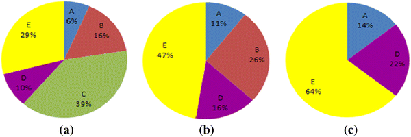
Roulette wheel representing the selection probabilities of chromosomes
- Step 6:
-
Spin the roulette wheel once and select one chromosome for the next generation
- Step 7:
-
Delete the selected chromosome in Step 6 from the updated population pool
- Step 8:
-
Update the population pool and Go to Step 3
- Step 9:
-
Repeat Steps 3–8 until the number of the selected chromosome equals the population size

Figure 1 illustrates the changes in selection probabilities of the chromosomes when the size of population pool is changed. In Fig. 1a, there are 5 chromosomes to be chosen for the next generation: A, B, C, D, and E. It can be seen that the chromosome C is the best one with the selection probability of 39%. It is a good idea to select the best one first to make sure it passes to the next generation as it has the highest potential to make a difference. After chromosome C has been selected and removed from the population pool, there are 4 chromosomes to be chosen from and their selection probabilities are as shown in Fig. 1b. Now, this roulette wheel is spun and one chromosome, say chromosome B, is selected for the next generation. Figure 1c presents the selection probabilities of 3 chromosomes after chromosome B is selected and removed from the population pool. As a result, the selection probability of chromosome A, for example, is increased from 6 to 11 or 14%. Clearly, the selection probabilities of the chromosomes are changing and the effect of super chromosomes can be eased as each chromosome can be selected only once, no matter how good it is.
The proposed selection approach has two advantages. The first one is that it can prevent super chromosomes from dominating population by maintaining too many copies in the population which causes the premature convergence to local optimum. The second one is that it is able to maintain the diversity of population in probability fashion so that the population pool can contain much more valuable information for genetic search.
Structure of the proposed genetic algorithm
To improve the search capability, the structure of the proposed GA is developed as shown in Fig. 2. It should be noted that, in the Fig. 2, g is the number of generations in each civilization; r is the number of good chromosomes selected for the next civilization; and c is the number of civilizations of the GA. In the first civilization, the initial population is totally generated randomly. In the other civilization, a part of the initial population is randomly generated and the rest is adopted from the previous civilization. With this structure, the proposed GA is capable of “learning” from its experience. From the second civilization, the GA has little “intelligence” so that it does not have to start the blind searching at the beginning while it still has ability to explore the wide search space. In addition, parameters of the proposed GA: population size (p), rate of the crossover 1 (c 1), rate of the crossover 2 (c 2), rate of the mutation 1 (m 1), rate of the mutation 2 (m 2), number of generations in each civilization (g) and number of good chromosomes selected for the next civilization (r) are tuned by Taguchi Experimental Design.

Structure of the proposed GA
Case study
To demonstrate the capability of the proposed GA, the case study in references (Dao and Marian 2011c, 2013) is adopted here and restated as follows.
Problem description
A manufacturing company having three different production lines is able to produce 50 different products, say P1, P2,…, P50, in the next month. Information about the products is detailed in Table 12. Resources available for the next month will be 800 h of labour, 1000 kg of material, and $1700 K of working capital.
Additionally:
-
Apart from the producing cost, overheads for running a production line also costs $300/h to be paid from the working capital.
-
Any product changeover takes 0.5, 1 and 1.5 h in production line 1, 2 and 3, respectively.
-
Any product made after the deadline incurs a penalty of 5% of the initial price per day of delay.
-
Any product made before its deadline contributes 10 points to the company’s customer satisfaction index.
-
Any product made after the deadline for more than 10 days will not be accepted by the customer and it will be returned to the company.
-
Each day after the deadline of any product incurs a penalty of 1 point of customer satisfaction index.
-
The proceedings from selling products will only be available for next month, so they should be ignored for the current planning horizon-current month.
-
The company can select any mix of products to produce in the next month, as long as its selection contains at least 20 different ones.
-
The company can work 24 h/day, 7 days/week.
The problem is to do the planning and scheduling for next month by (1) selecting what type of product to produce, (2) determining how many products in each selected type to produce, (3) allocating the selected products to which production line, and (4) selecting the manufacturing sequences of the selected products in three production lines to maximize the profit of the company as well as its customer satisfaction index while satisfying simultaneously all constraints described above. It should be noted that the weight coefficients of the two objective functions, total profit and customer satisfaction index, were assumed to be 0.7 and 0.3, respectively.
Results and discussions
The case study problem as described above was solved by the proposed GA. Taguchi Experimental Design based method was used to select the parameters of the proposed GA. Taguchi Orthogonal Array Design (L27–37) generated by Minitab software and the related experimental data are shown in Table 13. It is noted that to make a fair comparison, the proposed GA in any experiment was run for exactly the same computing time. In addition, to obtain the consistent experimental result, each experiment was repeated for three times. ANOVA analysis carried out in Minitab has revealed the effects of the seven parameters on the performance of the proposed GA as shown in Table 14 and Fig. 3. Based on the results in Table 14 and Fig. 3, the parameters of the proposed GA were chosen as shown in Table 15.

Effects of the parameters on the performance of the proposed GA
Three commercial optimisation solvers: Pattern Search (PS solver), Simulated Annealing (SA solver) and Genetic Algorithm (GA solver) in Matlab were used herein as the benchmarks to verify the effectiveness of the proposed GA. The three solvers were used to solve exactly the same case study problem and their performances are compared to one of the proposed GA as shown in Table 16 and Fig. 4. It is noted that the parameters of the solvers are set by default and unit of the computing time in Table 16 is minute. It can be seen from Table 16 that the computing time of the proposed GA is 35.4, 87.7 and 43.0% smaller compared to those of PS solver, SA solver and GA solver, respectively. More importantly, the proposed GA also outperforms the three commercial optimisation solvers in term of the solution quality. On average, the proposed GA provides 27.3, 62.3 and 80.2% better solution compared to PS solver, SA solver and GA solver, respectively. In term of consistency of the solution quality, the solvers as well as the proposed GA are about the same indicated by the standard deviation values shown in Table 16 and Fig. 4.

Comparison in terms of the solution quality
As can be seen from Table 16, the best solution to the case study problem found by the proposed GA is the one with the fitness value of 18033.7, which is 26.2% better than the solution already published by Dao and Marian (2011c, 2013). Detail of the best solution to the case study problem ever achieved is shown in Table 17. In addition, a typical evolution of the solution quality found by the proposed GA is shown in Fig. 5. It can be seen from Fig. 5 that the solution can be convergent to the optimal one after a few civilizations.

A typical evolution of the solution quality found by the proposed GA
The experimental results revealed that the proposed structure of GA is better than the conventional one; that is because it allows the GA to “learn” for its experience. From the second civilization, the GA does not have to start the totally blind searching at the beginning because it has adopted some best chromosomes for the previous civilization. However, the question is how many chromosomes should be migrated to the next civilization. If this number is large, the exploration of the GA will be limited. As a result, the probability of getting stuck in local optimums will increase. Whereas, if the number is small, the evolution process will be slow and sometimes valuable chromosomes will be lost. In this case study problem, the number found by Taguchi Experimental Design is 5 (r = 5) meaning that top 5 chromosomes from the previous civilization should be migrated to the next one. However, in other cases, 5 chromosomes might not be an optimal number. And this number should be selected, case by case, based on experimental information.
It can be seen from Table 16 that the optimization process, done by both the commercial optimisation solvers and the proposed GA, takes very long time and the consistency of the solution quality is not very high. There are two reasons for the problems. The first one is that the search space of the problem is huge as it involves 59 variables (9 variables in the resource allocation part plus 50 variables in the manufacturing sequence part) and more than 50!/(50–20)! possible combinations of the variables. The second one is that a large number of calculations are required to deal with a lot of complex constraints in the chromosome generating, crossover, mutation, evaluation processes. Super computers and parallel computing techniques are some promising tools to reduce the computing time and to achieve better solutions, especially when solving large-scale problems.
Conclusion and future work
In this paper, a novel GA has been developed to deal with multidimensional optimization for fully integration of production planning and scheduling associated with precedence constraints. As fully integration of the planning and scheduling, the proposed approach has highest potential to search for global solution. In addition, with the developed algorithm structure, variable-length chromosome, modified genetic operations, and algorithm parameters tuned by Taguchi Experimental Design, the proposed GA can deal with the integrated optimisation problem very effectively.
The robustness of the proposed GA has been validated in the comprehensive case study problem in which the proposed GA outperforms three commercial optimisation solvers in both computing time and solution quality. Moreover, the best solution to the case study problem found by the proposed GA is 26.2% better compared to the one which has been already published in the literature. In addition, the proposed GA is very general and it can easily accommodate much larger and more complex problems.
Further work should be conducted in the following areas:
-
Developing the GA for extended problem, e.g., adding more constraints such as variety of materials used, different product changeover for different pairs of products, etc.
-
Incorporation of stochastic events into the model and investigating their influence on the optimality.
-
Developing the computing technique to shorten the processing time.
-
Further validating the effectiveness of the proposed GA by comparing it with other approaches such as GAMS or other optimization software.
References
Abtahi AR, Bijari A (2016) A novel hybrid meta-heuristic technique applied to the well-known benchmark optimization problems. J Ind Eng Int 1–13 doi:10.1007/s40092-016-0170-x
Cadoli M et al (2000) NP-SPEC: an executable specification language for solving all problems in NP. Comput Lang 26(2–4):165–195
Dao SD, Marian R (2011) Optimisation of precedence-constrained production sequencing and scheduling using genetic algorithms. In The IAENG International Conference on Artificial Intelligence and Applications. Hong Kong, pp 59–64
Dao SD, Marian R (2011) Modeling and Optimization of Precedence-Constrained Production Sequencing and Scheduling Using Multi-Objective Genetic Algorithm. In International Conference of Computational Intelligence and Intelligent Systems. London, pp 1027–1032
Dao SD, Marian R (2011c) Modeling and Optimisation of Precedence-Constrained Production Sequencing and Scheduling for Multiple Production Lines Using Genetic Algorithm. Computer Technology and Application 2(6):487–499
Dao SD, Marian R (2013) Genetic Algorithms for integrated optimisation of precedence-constrained production sequencing and scheduling. In: Ao SI, Gelman L (eds) Electrical engineering and intelligent systems. Springer, New York, pp 65–80
He K, Huang W, Jin Y (2012) An efficient deterministic heuristic for two-dimensional rectangular packing. Comput Oper Res 39(7):1355–1363
Javanmard H, Koraeizadeh AAW (2016) Optimizing the preventive maintenance scheduling by genetic algorithm based on cost and reliability in National Iranian Drilling Company. J Ind Eng Int 12:1–8. doi:10.1007/s40092-016-0155-9
Kim YK, Park K, Ko J (2003) A symbiotic evolutionary algorithm for the integration of process planning and job shop scheduling. Comput Oper Res 30(8):1151–1171
Liu Y, Fang Y (2012) Boost the Integration of planning and scheduling: a heuristics approach. Proc Eng 29:3348–3352
Maravelias CT, Sung C (2009) Integration of production planning and scheduling: Overview, challenges and opportunities. Comput Chem Eng 33(12):1919–1930
Marian R, Luong LHS, Akararungruangkul R (2008a) Optimisation of distribution networks using Genetic Algorithms. Part 1-problem modelling and automatic generation of solutions. Int J Manuf Technol Manage 15(1):64–83
Marian R, Luong LHS, Akararungruangkul R (2008b) Optimisation of distribution networks using Genetic Algorithms. Part 2-the Genetic Algorithm and Genetic Operators. Int J Manuf Technol Manage 15(1):84–101
Moradgholi M et al (2016) A genetic algorithm for a bi-objective mathematical model for dynamic virtual cell formation problem. J Ind Eng Int 12(3):343–359. doi:10.1007/s40092-016-0151-0
Shao X et al (2009) Integration of process planning and scheduling—a modified genetic algorithm-based approach. Comput Oper Res 36(6):2082–2096
Shapiro M, Delgado-Eckert E (2012) Finding the probability of infection in an SIR network is NP-Hard. Math Biosci 240(2):77–84
Acknowledgements
The first author is grateful to Australian Government for sponsoring his PhD study at the University of South Australia, Australia in form of Endeavour Award.
Author information
Authors and Affiliations
Corresponding author
Rights and permissions
Open Access This article is distributed under the terms of the Creative Commons Attribution 4.0 International License (http://creativecommons.org/licenses/by/4.0/), which permits unrestricted use, distribution, and reproduction in any medium, provided you give appropriate credit to the original author(s) and the source, provide a link to the Creative Commons license, and indicate if changes were made.
About this article

Cite this article
Dao, S.D., Abhary, K. & Marian, R. An improved genetic algorithm for multidimensional optimization of precedence-constrained production planning and scheduling. J Ind Eng Int 13, 143–159 (2017). https://doi.org/10.1007/s40092-016-0181-7
Received:
Accepted:
Published:
Issue Date:
DOI: https://doi.org/10.1007/s40092-016-0181-7