
Abstract
Biological measurements are a rich source of information about the biological phenomena that are represented. For example, time-series dynamic genomic or metabolic microarray data can be used to construct dynamic genetic regulatory network models, which can be used to better understand the interactions among different genes within the biological system and to design intervention strategies to cure or manage major diseases. Unfortunately, biological measurements are usually highly contaminated with errors that mask the important features in the data and limit their applicability. Therefore, these noisy measurements need to be filtered to enhance their usefulness in practice. In this work, various model-based and model-free data filtering techniques are used to denoise (or filter) genomic data. In the availability of a dynamic model representing the biological system, state estimation techniques, such as extended Kalman filtering (EKF), unscented Kalman filtering (UKF), and particle filtering (PF) are used to filter the measured data. When a model is not available, on the other hand, low-pass as well as multiscale filtering techniques will be utilized. Low-pass filters include the mean and exponentially weighted moving average filters, while the multiscale filters include several online as well as batch wavelet-based thresholding techniques. In this paper, the performances of all filtering techniques will be demonstrated and compared through their application using simulated time-series metabolic data contaminated with white noise. The results show clear advantages for the model-based over the model-free filtering techniques, and that the PF outperforms other model-based methods. The results also show that in the absence of a model of the biological system, the model-free filtering techniques, especially multiscale filtering, can also provide acceptable performances. Online multiscale (OLMS) filtering is shown to outperform low-pass filtering, and the batch multiscale methods, i.e., translation invariant (TI) and boundary corrected TI (BCTI) provide enhanced smoothness, with improved ability of BCTI over TI at the edges. From a biological perspective, the model-based and online model-free filtering techniques can be used when filtering is needed online, such as within an intervention framework to cure diseases, while the batch model-free filtering techniques can be used within a modeling framework to enhance the quality of the estimated biological models.
1 Introduction
Recent advances in the DNA sensing technologies allowed the collection of microarray genomic and metabolic data from various biological systems. These data are a valuable source of information about the biological systems they are collected from. For example, the availability of time-series dynamic genomic or metabolic data has made it possible to construct dynamic models that can not only be used to characterize the behavior of such biological systems and the interactions among different genes (Jong 2002; Chou et al. 2006; Gonzalez et al. 2007; Kutalik et al. 2007; Wang et al. 2009, 2010; Meskin et al. 2011; Zhou et al. 2012; Huang et al. 2009; Qiu and Plevritis 2011; Noor et al. 2012), but also to design intervention strategies for curing/managing major disease phenotypes (Ervadi-Radhakrishnan and Voit 2005; Meskin et al. 2011; Nounou et al. 2012; Meskin et al. 2012). Unfortunately, biological data are usually contaminated with measurement noise that can greatly degrade the usefulness of the data (Hulse et al. 2012). For example, constructing a dynamic genetic regulatory network model using noisy time-series biological data will not only affect the accuracy of the estimated model, but also the effectiveness of any intervention technique that can be developed based on that model (Kutalik et al. 2007). This means that measurement errors in biological data need to be filtered to reduce the noise content and enhance the usefulness of these data in practice. The applicability of genomic and metabolic data in modeling and intervention biological phenomena is schematically illustrated in Fig. 1.

A schematic diagram illustrating the applicability of metabolic data in practice
Generally, data filtering techniques can be classified into three main categories: filtering with a model, filtering with an empirical model, and filtering without a model. The model-based filtering techniques rely on minimizing the error between the measured and filtered data while requiring the filtered data to satisfy the available model. Methods in this category include Kalman filtering (Sorenson 1985), Moving Horizon Estimation, and particle filtering (PF) (Gustafsson et al. 2002; Arulampalam et al. 2002; Rawlings and Bakshi 2006). For nonlinear processes, different versions of Kalman filters have been developed, which include the extended Kalman filter (EKF) (Simon 2006; Grewal and Andrews 2008; Julier and Uhlmann 1997; Ljung 1979; Kim and Park 1994) and the unscented Kalman filter (UKF) (Simon 2006; Grewal and Andrews 2008; Kim and Park 2000, 2001; Kim et al. 2007). In the EKF, the model describing the system is linearized at every time sample (to estimate the mean and covariance matrix of the state vector), and thus, the model is assumed to be differentiable. Unfortunately, for highly nonlinear or complex models, the EKF does not usually provide a satisfactory performance. On the other hand, instead of linearizing the model to approximate the mean and covariance matrix of the state vector, the UKF uses the unscented transformation to improve the approximation of these moments. In the unscented transformation, a set of samples (called sigma points) are selected and propagated through the nonlinear model, which provides more accurate approximations of the mean and covariance matrix of the state vector, and thus, results in a more accurate state estimation. Both EKF and UKF have been used in modeling biological systems and in designing intervention techniques that can be used in treating diseases (Meskin et al. 1979, 2011). The PF, on the other hand, is an implementation of a recursive Bayesian estimator (Gustafsson et al. 2002; Arulampalam et al. 2002), which relies on approximating the posterior (which is the density function of the unobserved state vector given a sequence of the observed data) as a set of random samples called particles. The advantage of the PF is that it is not restricted to linear and Gaussian processes, which makes it applicable in a wide range of applications. Of course, in all the model-based filtering techniques, the quality of the estimation depends on the accuracy of the models used.
A major challenge when dealing with biological systems is that models are not usually available a priori. This is because of the scarcity and the quality of the available biological data. In the absence of a fundamental model and in the case of multivariate filtering, an empirical model that is extracted from the relationship between the measured variables can also be used in data filtering. Methods in this category include Principal Component Analysis (PCA) (Kramer and Mah 1994). Since accurate process models are usually not available, the most widely used filtering methods do not rely on fundamental or empirical models; instead, they rely on information about the nature of the errors or the smoothness of the underlying signal. Examples of model-free filters include the well-known low-pass filters, such as the Finite Impulse Response (FIR) and Infinite Impulse Response (IIR) filters (Tham and Parr 1994). Examples of FIR and IIR filters include the mean filter (MF) and the exponentially weighted moving average (EWMA) filter, respectively. These are very popular filters as they are computationally efficient and can be implemented online. However, they are not very effective when used to filter data containing features with varying contributions over time and frequency. This is because low-pass filters define a frequency threshold above which all features are considered noise. Therefore, they may eliminate important features having higher frequencies than the threshold value and retain noise components that are changing at lower frequencies than the threshold value. An example of a high frequency feature is a sharp change in the data, while an example of low frequency noise is correlated (or colored) measurement errors. Thus, filtering the practical biological data that may contain features spanning wide ranges in time and frequency requires multiscale filtering algorithms that can account for this multiscale nature of the data.
Wavelet-based multiscale representation of data has been widely used in the analysis and investigation of various biological systems. For example, wavelets have been used to analyze genomic or DNA sequences to detect specific patterns (Arneodo et al. 1996, 1998; Dodin et al. 2000; Li 2003; Huang et al. 2008; Nguyen 2010). Also, wavelets have been applied to various aspects of protein structural investigations, including secondary and tertiary structure determination (Murray et al. 2002), refinement of X-ray crystallography (Main and Wilson 2000), and drug design and visualization (Mandell et al. 1998). Moreover, wavelets have been used in the analysis of microarray data and functional magnetic resonance imaging (fMRI) data (Dinov et al. 2005). Other applications of wavelets in biological systems include the analysis of 3-D biological shapes using conformal mapping and spherical wavelets. Wavelet-based filtering has also been used to denoise biological data. The authors in (Prasad et al. 2008) developed a new thresholding filter to be used in multiscale denoising of biological signals, and the authors in (Ustndag et al. 2012) used wavelet analysis and fuzzy thresholding in ECG data filtering.
In this work, various model-based as well as model-free filtering techniques will be compared when applied to filter time-series biological data representing dynamic metabolic measurements corresponding to four different genes. The model-based filtering techniques include the EKF, the UKF, and the PF. The model-free techniques include various low-pass filtering as well as several multiscale filtering techniques. Examples of low-pass filtering methods include MF and EWMA filtering. Examples of multiscale filtering methods, on the other hand, include standard multiscale (SMS) filtering, online multiscale (OLMS) filtering, translation invariant (TI) filtering, and boundary corrected TI (BCTI) filtering.
The remainder of this paper is organized as follows. In Sect. 2, a statement of the model-based filtering problem is presented followed by descriptions of some of the state estimation techniques used to solve this filtering problem. Then, in Sect. 3, a brief description of some of the low-pass filtering techniques is presented, followed by a description of multiscale representation of data and some of the multiscale filtering methods. Then, in Sect. 4, the various model-based and model-free filtering methods are compared using simulated time-series metabolic data. Finally, concluding remarks are presented in Sect. 5.
2 Model-based filtering
In this section, a problem statement of model-based filtering of biological data is presented, followed by descriptions of some the state estimation techniques that can be used to solve it.
2.1 Problem statement
Let the changes in the concentrations of various metabolites or proteins in a biological system be described by the nonlinear state space model described below:
where \({x\in \mathbb{R}^{n}}\) is a vector of the state variables (concentrations of certain metabolite inside the cell), \({u \in \mathbb{R}^p}\) is a vector of the input variables (any manipulated variables that can change the state variables), \({\theta \in \mathbb{R}^q}\) is a known parameter vector, \({y \in \mathbb{R}^m}\) is a vector of the measured variables (measured metabolite concentrations), \({w \in \mathbb{R}^{n}}\) and \({v \in \mathbb{R}^{m}}\) are process and measurement noise vectors, respectively, and g and l are nonlinear differentiable functions that describe the changes in the state variables over time. Discretizing the state space model (1), the discrete model can be written as follows:
which quantifies the state variables at some time step (k) in terms of their values at a previous time step (k − 1). In Eq. (1), the two nonlinear functions \({\mathfrak{F}}\) and \({\mathfrak{R}}\) are the equivalent functions to the functions g and l, but for the discrete model. Let the process and measurement noise vectors have the following properties: \(\mathbf{E}[w_k]=0, \mathbf{E}[w_k w_k^T]=\mathbf{Q}_k, \mathbf{E}[v_k]=0\) and \(\mathbf{E}[v_k v_k^T]=\mathbf{{R}}_k, \) where \(\mathbf{Q}_k\) and \(\mathbf{R}_k\) are the covariance matrices of the process and measurement noise vectors, respectively. The objective here is to estimate the state vector x k , given the measurements vector y k . Some of the techniques that can be used to solve this state estimation (filtering) problem are presented next.
2.2 Description of state estimation techniques
In this section, the formulations as well as the algorithms of some of the state estimation techniques (which include EKF, UKF, and PF) will be presented.
-
1.
Extended Kalman filtering (EKF): As the name indicates, EKF is an extension of Kalman filtering (KF) (Lee and Ricker 1994), where the model is linearized to estimate the covariance matrix of the state vector. As in KF, the state vector x k is estimated by minimizing a weighted covariance matrix of the estimation error, i.e., \(\mathbf{E}[({x}_k-\widehat{x}_k)\mathbf{M}({x}_k-\widehat{x}_k)^T], \) where \(\mathbf{M}\) is a symmetric nonnegative definite weighting matrix. If all the states are equally important, \(\mathbf{M}\) can be taken as the identity matrix, which reduces the covariance matrix to \(\mathbf{P}=\mathbf{E}[({x}_k-\widehat{x}_k)({x}_k-\widehat{x}_k)^T]. \) Such a minimization problem can be solved by minimizing the following objective function:
$$ {\mathbf{J}}=\frac{1}{2}Tr\Bigl({\mathbf{E}}[({x}_k-\widehat{x}_k)({x}_k-\widehat{x}_k)^T]\Bigr). $$(3)subject to the model defined in Eq. (2). To minimize the above objective function (3), EKF estimates the state vector using a two-step algorithm: prediction and estimation (or update), which are described next (refer to Algorithm 1).
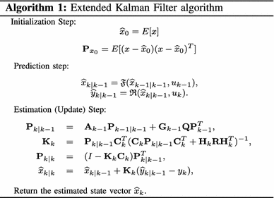 In Algorithm 1, \(\mathbf{P}_{{k}|{k-1}}\) is the innovation (or residual) covariance matrix, \(\mathbf{K}_{{k}}\) is the near-optimal Kalman filter gain matrix, \(\mathbf{P}_{{k}|{k}}\) is the updated covariance matrix, and \(\widehat{x}_{{k}|{k}}\) is the updated state estimate. In addition, the state transition and observation matrices are defined to be the following Jacobians, \({\mathbf{A}_{k-1} \approx \frac{\partial \mathfrak{F}}{\partial x}|_{\widehat{x}_{{k-1}|{k-1}}}, \mathbf{C}_{k-1} \approx \frac{\partial \mathfrak{R}}{\partial x}|_{\widehat{x}_{{k-1}|{k-1}}}, \mathbf{G}_{k-1} \approx \frac{\partial \mathfrak{F}}{\partial \epsilon}|_{\epsilon_{k-1}}}\) and \({\mathbf{H}_{k} \approx \frac{\partial \mathfrak{R}}{\partial v}|_{v_{k}}, }\) which are the matrices of the linearized system model at every time step.
 -
2.
Unscented Kalman filtering: for highly nonlinear systems, the EKF may not provide a satisfactory performance because EKF approximates the mean and covariance matrix of the nonlinear state vector by linearizing the nonlinear model, which may not provide good approximations of these moments. To enhance the estimation of the mean and covariance matrix of the state vector, the UKF, which relies on the unscented transformation, has been developed (Simon 2006; Grewal and Andrews 2008; Kim and Park 2000, 2001; Kim et al. 2007). The unscented transformation is a method for calculating the statistics of a random variable which undergoes a nonlinear mapping (Julier and Uhlmann 1997). Assume that a random variable \({x \in \mathbb{R}^{r}}\) with mean \(m_x=\mathbf{E}[({x}_k-\widehat{x}_k)\mathbf{M}({x}_k-\widehat{x}_k)^T]\) and covariance matrix \(\mathbf{P}_x\) is transformed by a nonlinear function, y = f(x). To find the statistics of y, 2r + 1 sigma vectors are defined as follows (Van Der Merwe et al. 2001):
$$ \begin{aligned} &X_0=\overline{x} \\ &X_i=\overline{x}+(\sqrt{(r+\lambda){\mathbf{P}}_x})_i\quad i=1,...,r \\ &X_i=\overline{x}-(\sqrt{(r+\lambda){\mathbf{P}}_x})_i \quad i=r+1,...,2r \\ \end{aligned} $$(4)where, λ = e 2(r + k) − r is a scaling parameter and \((\sqrt{(r+\lambda)\mathbf{P}_x})_{i}\) denotes the ith column of the matrix square root of \((r+\lambda)\mathbf{P}_x. \) The constant 10−4 < e < 1 determines the spread of the sigma points around \(\overline{x}, \) and the constant k is a secondary scaling parameter which is usually set to zero or 3 − r (Julier and Uhlmann 1997). Then, these sigma points are propagated through the nonlinear function, i.e.,
$$ Y_i=f({X}_i)\quad i=0,...,2r $$(5)and the mean and covariance matrix of y can be approximated as weighted sample mean and covariance of the transformed sigma points of Y i as follows:
$$ \begin{aligned} \overline{y} &\approx \sum_{i=0}^{2r}{W_i^{(m)}Y_i}, \\ \hbox {and } {\mathbf{P}}_x &\approx \sum_{i=0}^{2r}{W_i^{(c)}(Y_i-\overline{y})(Y_i-\overline{y})^T}, \\ \end{aligned} $$(6)where, the weights are given by:
$$ \begin{aligned} &W_i^{(m)}= \frac{\lambda}{\lambda+r},\\ &W_0^{(c)}= \frac{\lambda}{\lambda+r}+(1-e^2+\xi), \\ \text {and}\; &W_i^{(m)}= W_i^{(c)}=\frac{1}{2(\lambda+r)},\quad i=0,...,2r. \end{aligned} $$(7)The parameter ξ is used to incorporate prior knowledge about the distribution of x. It has been shown that for a Gaussian and non-Gaussian variables, the unscented transformation results in approximations that are accurate up to the third and second order, respectively (Wan and Van Der Merwe 2001). Based on this unscented transformation, the unscented Kalman filtering algorithm can be summarized as shown in Algorithm 2.
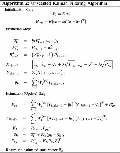 In Algorithm 2, \(\widehat{x}_{0}\) is the initial estimate, \(\mathbf{P}_{{x}_{0}}\) is the initial covariance matrice, \(\widehat{x}_{k}^- \) is the predicted state, \(P_{{xk}}^{ - } \) is the predicted covariance matrix, X
k|k−1 is the sigma point, Y
k|k−1 is the projected sigma point through the observation function, \(\widehat{y}_{k}\) is the predicted output, P
yk
is the updated output cross-covariance matrix, P
xk
,
yk
is the state-measurement covariance matrix, K
k
is the UKF Kalman filter Gain, \(\widehat{x}_{k}\) is the updated state vector, and P
xk
is the updated covariance matrix.
In Algorithm 2, \(\widehat{x}_{0}\) is the initial estimate, \(\mathbf{P}_{{x}_{0}}\) is the initial covariance matrice, \(\widehat{x}_{k}^- \) is the predicted state, \(P_{{xk}}^{ - } \) is the predicted covariance matrix, X
k|k−1 is the sigma point, Y
k|k−1 is the projected sigma point through the observation function, \(\widehat{y}_{k}\) is the predicted output, P
yk
is the updated output cross-covariance matrix, P
xk
,
yk
is the state-measurement covariance matrix, K
k
is the UKF Kalman filter Gain, \(\widehat{x}_{k}\) is the updated state vector, and P
xk
is the updated covariance matrix. -
3.
Particle filtering: a PF is an implementation of a recursive Bayesian estimator (Gustafsson et al. 2002; Arulampalam et al. 2002). Bayesian estimation relies on computing the posterior p(x k |y 1:k ), which is the density function of the unobserved state vector, x k , given a sequence of the observed data \(y_{1:k} \equiv \{y_1,\; y_2,\;\cdots,\; y_k\}. \) However, instead of describing the required posterior distribution in a functional form, in PF, it is represented approximately as a set of random samples of the posterior distribution. These random samples, which are called the particles of the filter, are propagated and updated according to the dynamics and measurement models (Doucet and Johansen 2009; Arulampalam et al. 2002). The advantage of the PF is that it is not restricted by the linear and Gaussian assumptions, which makes it applicable in a wide range of applications. The basic form of the PF is also simple, but may be computationally expensive. Thus, the advent of cheap, powerful computers over the last decade has been a key to the introduction and utilization of PF in various applications.
 In Algorithm 1,
  In Algorithm 2,
 For a given dynamical system describing the evolution of the states and parameters that we wish to estimate, the estimation problem can be viewed as an optimal filtering problem (Andrews et al. 2006), in which the posterior distribution, p(x k |y 1:k ), is recursively updated. Here, the dynamical system is characterized by a Markov state evolution model, p(x k | x 1:k−1) = p(x k | x k−1), and an observation model, p(y k |x k ). In a Bayesian context, the task of state estimation can be formulated as recursively calculating the predictive distribution p(x k |y 1:k−1) and the filtering distribution p(x k |y 1:k ) as follows,
The state vector x k is assumed to follow a Gaussian model, \(x_{k} \thicksim \mathcal{N}(\mu_{k},\lambda_{k}). \) Thus, the marginal state distribution is obtained by integrating over the mean and covariance matrix as follows,
where the integration with respect to the covariance matrix leads to the known class of scale mixture distributions introduced by Barndorff-Nielsen (1977) for the scalar case.
The nonlinear nature of the system model leads to intractable integrals when evaluating the marginal state distribution, p(x k |x k−1). Therefore, Monte Carlo approximation is utilized, where the joint posterior distribution, p(x 0:k |y 1:k ), is approximated by the point-mass distribution of a set of weighted samples (particles) \( \left\{ {x_{{0:k}}^{{(i)}} ,\ell _{k}^{{(i)}} } \right\}_{{i = 1}}^{N} ,\) i.e.,:
where \(\delta_{ x^{(i)}_{0:k}} (d x_{0:k})\) denotes the Dirac function, and N is the total number of particles. Based on the same set of particles, the marginal posterior probability of interest, p(x k |y 1:k ), can also be approximated as follows:
In this Bayesian importance sampling (IS) approach, the particles \( \left\{ {x_{{0:k}}^{i} } \right\}_{{i = 1}}^{N} \)are sampled from the following distribution,
Then, the estimate of the state vector \(\widehat{x}_{k}\) can be approximated by a Monte Carlo scheme as follows:
where \( \ell _{k}^{{(i)}} \) are the corresponding importance weights, which are defined as follows:
A common problem with the sequential IS-based PF is the degeneracy phenomenon, where after a few iterations, all but one particle will have negligible weights. It has been shown (Yang et al. 2005) that the variance of the importance weights can only increase over time, and thus, it is impossible to avoid the degeneracy phenomenon. This degeneracy implies that a large computational effort is devoted to update the particles whose contributions to the approximation of p(x k |y 0:k ) are almost zero. A suitable measure of degeneracy of the algorithm is the effective sample size N eff, which is introduced in (Gustafsson et al. 2002) and (Liu and Chen 1998), and is defined as,
where \( \ell _{k}^{{(i)}} \) are the normalized weights obtained using (14). State estimation using PF can be summarized as shown in Algorithm 3.
The state estimation techniques described earlier (EKF, UKF, and PF) utilize a model of the biological system to filter (or provide better estimates of) the measured metabolic or genomic data. When a model is not available, however, model-free filtering of these data can be used. Some of the univariate model-free data filtering techniques that can be used in this regard are described next.
3 Model-free filtering
In the absence of a model of the biological system, which is common due to the complexity of biological phenomena, measured biological data can be filtered using univariate filtering techniques that rely on information about the errors or assumptions about the nature of the noise-free data. Some of these filtering techniques include linear low-pass filtering and multiscale filtering, which are described next.
3.1 Linear data filtering
Linear filtering techniques filter the data by computing a weighted sum of previous measurements in a window of finite or infinite length. These techniques include FIR and IIR filters, which are popular because they are computationally efficient and can be implemented online (Tham and Parr 1994). A linear filter can be written as follows,
where, b i is the ith filter coefficient, \(\sum_i {b_i }=1, N\) is the filter length, x k is the measured variable (such as a metabolite concentration) and \(\hat x_k\) is the filtered value of the variable. A well-known FIR filter is the MF, where \( b_i=\frac{1}{N}. \) An example of an IIR filter, on the other hand, is the EWMA filter, which can be expressed as follows,
where, α is a smoothing parameter between 0 and 1, where a value of one corresponds to no filtering and a value of zero corresponds to only keeping the first measured data point. A more detailed discussion of different types of linear filters is presented in (Strum and Kirk 1989).
In linear filtering, the basis functions representing raw measured data have a temporal localization equal to the sampling interval. This means that linear filters are single-scale in nature, since all the basis functions have the same fixed time–frequency localization. Consequently, these methods face a trade-off between accurate representation of temporally localized changes and efficient removal of temporally global noise. Therefore, simultaneous noise removal and accurate feature representation of the measured signals cannot be effectively achieved by single-scale filtering methods (Nounou and Bakshi 1999). Enhanced denoising can be achieved using multiscale filtering as will be described next.
3.2 Multiscale data filtering
In this section, several multiscale filtering methods are described. However, since multiscale filtering relies on multiscale representation of data using wavelets and scaling functions, a brief introduction to multiscale representation will be presented first.
(1) Multiscale representation of data: A signal can be represented at multiple resolutions by decomposing it, using a family of wavelets and scaling functions. Consider the time-series measurements of the concentration of a particular metabolite in a biological system which are shown in Fig. 2a (see the description of the biological system in Sect. 4). The signals in Fig. 2b, d, f are at increasingly coarser scales compared to the original signal in Fig. 2a, and are called scaled signals. These scaled signals are determined by projecting the original signal on a set of orthonormal scaling functions of the form,
or equivalently by filtering the signal using a low-pass filter of length \(r, h_{f}=\left[ {h_1 ,h_2 ,..,h_r } \right], \) derived from the scaling functions. On the other hand, the signals in Fig. 2c, e, g, which are called the detail signals, capture the details between any scaled signal and the scaled signal at the finer scale. These detailed signals are determined by projecting the original signal on a set of wavelet basis functions of the form,
or equivalently by filtering the scaled signal at the finer scale using a high-pass filter of length r, g f = [g 1, g 2, .., g r ], derived from the wavelet basis functions. Therefore, the original signal can be represented as the sum of all detail signals at all scales and the scaled signal at the coarsest scale as follows,
where j, k, J, and n are the dilation parameter, translation parameter, maximum number of scales (or decomposition depth), and the length of the original signal, respectively (Strang 1989; Daubechies 1988; Mallat 1989), and a Jk is the kth scaling coefficient at scale J and d jk is the kth wavelet coefficient at the jth scale.

A schematic diagram of data representation at multiple scales
(2) Standard multiscale (SMS) filtering: Multiscale filtering using wavelets is based on the observation that random errors in a signal are present over all wavelet coefficients, while deterministic changes get captured in a small number of relatively large wavelet coefficients (Donoho and Johnstone 1994; Donoho et al. 1995; Bakshi 1999; Nounou and Bakshi 2000). Thus, stationary Gaussian noise may be removed by a three-step method (Donoho et al. 1995):
-
1.
Transform the noisy signal into the time–frequency domain by decomposing the signal onto a selected set of orthonormal wavelet and scaling basis functions.
-
2.
Threshold the wavelet coefficients by suppressing coefficients smaller than a selected value.
-
3.
Transform the thresholded coefficients back into the original time domain.
Donoho and coworkers have studied the statistical properties of wavelet thresholding and have shown that for a noisy signal of length n, the filtered signal will have an error within O(log n) of the error between the noise-free signal and the signal filtered with a priori knowledge about the smoothness of the underlying signal (Donoho and Johnstone 1994).
Selecting the proper value of the threshold is a critical step in this filtering process, and several methods have been devised. For good visual quality of the filtered signal, the Visushrink method determines the threshold as (Donoho and Johnstone 1994),
where, n is the signal length and σ j is the standard deviation of the errors at scale j, which can be estimated from the wavelet coefficients at that scale using the following relation,
Other methods for determining the value of the threshold are described in (Nason 1996).
(3) Translation invariant (TI) filtering: In SMS filtering, when the wavelet basis function used to represent a certain feature in the signal is not aligned with the feature itself, an artifact, which is not present in the original signal, can be created in the filtered signal. TI filtering is one approach that was proposed in (Coifman and Donoho 1995) to deal with this problem by shifting the signal several times, filtering it, and then averaging out all translations to suppress these artifacts and improve the smoothness of the filtered data (see Fig. 3). This approach, however, suffers from the creation of end effects because TI filtering considers the signal to be a cyclic signal, which results in artificial discontinuities when the two end points in the signal are very different in magnitude. This disadvantage can be overcome by the BCTI filtering method, which will be discussed in Sect. 3 (B.5).

A schematic diagram of the translation mechanism used in TI filtering
(4) OLMS filtering: The standard and TI multiscale filtering techniques described earlier are batch, i.e., they require the entire data set (which has to be of dyadic length) a priori, and thus, cannot be implemented online. When filtering time-series metabolic data, batch filtering would be acceptable if the filtered data are needed to estimate the parameters of a genetic regulatory network for example. However, if the filtered data are used within an intervention framework, then the metabolic data need to be filtered online as they are measured. To deal with this problem, an OLMS filtering algorithm, that is based on multiscale filtering of data in a moving window of dyadic length, has been developed (Nounou and Bakshi 1999). The OLMS algorithm is summarized below:
-
1.
Decompose the measured data within a window of dyadic length using a causal boundary corrected wavelet filter.
-
2.
Threshold the wavelet coefficients and reconstruct the filtered signal.
-
3.
Retain only the last data point of the reconstructed signal for online use.
-
4.
When new measured data are available, move the window in time to include the most recent measurement, while maintaining the maximum dyadic window length (as illustrated in Fig. 4).
Fig. 4 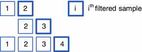
A schematic diagram of the moving window mechanism used in OLMS and BCTI filtering
Note from Fig. 4 that the moving window always seeks to keep the largest number of dyadic samples available, which would provide a more accurate estimation of the threshold value. Also, note that if a wavelet filter other than Haar is used in OLMS filtering, a boundary corrected version of the filter is needed to avoid inaccuracies at the boundaries. This is particularly important because OLMS only retains the last filtered data point from each window.

(5) BCTI Filtering: If all the filtered signals from all moving windows in OLMS (shown in Fig. 4) are averaged, a much smoother filtered signal is obtained. This is in fact similar to TI filtering, but since it does not assume the signal to be a cyclic list, it overcomes the problem of boundary effects encountered in TI, and thus, is called BCTI. Another advantage is that BCTI averages less number of data points when computing the final estimated signals (compare the mechanisms of TI and BCTI in Figs. 3 and 4, respectively), and thus, BCTI is computationally less expensive than TI. The performances of all filtering techniques are illustrated and compared through a simulated case study.
4 Case study: filtering of dynamic genomic data
The objective behind this case study is twofold: first, highlight the applicability of data filtering for biological data; second, to compare the performances of various model-based and model-free filtering algorithms (which were discussed in this paper) through their application using simulated time-series metabolic data representing the concentrations of four metabolites that are related by the branched pathway shown in Fig. 5. These concentrations are the four dependent variables x 1, ..., x 4 in the following S-system (Voit and Almeida 2004), which also involves one independent variable x 5:

Generic branched pathway with four dependent variables
The four differential equations shown in model (23), describe the changes in the concentrations of four different metabolites within the cell, and thus, quantify the interactions among the genes responsible for producing these metabolites. We chose to use a biological phenomenon represented by an S-system model in this simulated example because the S-system model has a canonical nonlinear model structure that can capture the behavior of a large class of biological systems due to its ability to provide a good trade-off between accuracy and mathematical flexibility (Voit 1991; Gentilini 2005). The data used in this case study are generated by first discretizing the S-system (23) using a sampling time of 3.9 s, and then simulating the discretized model using the following initial conditions: x 1(0) = 5.6, x 2(0) = 3.1, x 3(0) = 2.9, and x 4(0) = 3.1, and assuming x 5 = 1. The simulated data, which are assumed to be noise-free, are then contaminated with additive zero mean Gaussian noise, i.e., the noisy data are computed simply by adding the noise to the noise-free data. Two levels (variances) of noise, which correspond to signal-to-noise ratios (SNR) of 10 and 20, are used to provide a good comparison between the performances of the different filtering techniques. The SNR is the ratio of the variance of the noise-free data to the variance of the added noise.
The model-based filtering techniques used in this case study include the EKF, the UKF, and the PF. The model-free filtering techniques, on the other hand, include MF, EWMA filtering, SMS filtering, TI filtering, and BCTI filtering. The filter parameters for all model-free filtering techniques are optimized using cross-validation (Nason 1996), where the data are split into two sets, odd and even. Then, each set (odd and even) is filtered separately, and then the following cross-validation mean square error is minimized to determine the optimum filter parameters:
where \(\bar x_{{\rm odd},k}=\frac{1}{2}\left({\hat x_{{\rm even},k + 1}+\hat x_{{\rm even},k}}\right), \bar x_{{\rm even},k}= \frac{1}{2}\left({\hat x_{{\rm odd},k+1}+\hat x_{{\rm odd},k}}\right), \) and \({\hat x_{{\rm odd},k}}\) and \({\hat x_{{\rm even},k}}\) are the kth odd and even filtered data samples, respectively, and N is the total number of data samples. The performances of the various filtering techniques are compared by computing the mean square error with respect to the noise-free data, i.e., \({\rm MSE}=\frac{1}{N} \sum \nolimits_{k=1}^N {\left({\hat x_k-\tilde x_k} \right)^2},\) where \(\hat x_k\) and \(\tilde x_k\) are the kth filtered and noise-free data samples, respectively.
To make statistically valid conclusions about the performances of all techniques, a Monte Carlo simulation using 1,000 realizations is performed. The results of the model-based filtering techniques are summarized in Table 1 and are illustrated in Fig. 6 for the case, where SNR = 10. The results of the model-free filtering techniques, on the other hand, are summarized in Table 2 and are illustrated in Figs. 7 and 8 also for the case, where SNR = 10. In all figures, x 1 is in blue, x 2 is in dark green, x 3 is in red, and x 4 is in light green.

Comparison between the performances of various model-based filtering methods for the case, where SNR = 10 (dashed lines noise-free, solid lines filtered)

Comparison between the performances of various online model-free filtering methods for the case, where SNR = 10 (dashed lines noise-free, solid lines filtered)

Comparison between the performances of various batch multiscale filtering methods for the case, where SNR = 10 (dashed lines noise-free, solid lines filtered)
Table 1 and Fig. 6 show that UKF performs better than EKF because UKF can provide more accurate estimation of the mean and covariance matrix of the state vector than EKF, which estimates these moments using a linearized model. The results also show that the PF by far outperforms all other model-based filtering techniques because of its ability to better handle nonlinear systems than EKF and UKF. These model-based filtering techniques can help within a model-based intervention framework, where a model is available. On the other hand, the results of the model-free filtering methods (summarized in Table 2) show that good noise-removal can still be archived without a model. The results show that OLMS filtering outperforms the conventional low-pass filters (MF and EWMA), which can all be implemented online. This advantage can be helpful if the filtered data are utilized in model-free intervention, such as fuzzy intervention in biological systems (Nounou et al. 2012). The advantages of OLMS can be clearly seen in Fig. 7. If more time is available to filter the data, other batch multiscale filtering methods can perform even better. For example, the SMS technique provides a clear improvement over all online methods, including OLMS, as demonstrated in Fig. 8. Other batch multiscale filtering techniques can provide improved smoothness, such as TI. However, due to the cycle-spinning of the data, TI results in boundary effects, especially if the two ends of the data are significantly different in magnitude, such as in the case of x 1 (in blue) and x 4 (in light green) in Fig. 8. This drawback of TI is accounted for in BCTI, which provides similar smoothness without the boundary effects, and thus, results in smaller mean square errors as shown in Table 2. The advantages of these batch multiscale filtering techniques can be helpful if the filtered biological data are used to enhance the accuracy of biological models which are estimated from these filtered data.
5 Conclusion
Data filtering is important to enhance the quality and usefulness of noisy biological data, which can be used to model biological phenomena and to design intervention techniques for treating diseases. This paper presented a comparison between various model-based and model-free filtering techniques when used to denoise biological data contaminated with measurement errors. The model-based filtering techniques used in this work include the (EKF, UKF, and PF). The model-free filtering techniques include various low-pass as well as multiscale filtering methods. Examples of low-pass filters include the MF and the EWMA filter, while examples of multiscale filters include the OLMS, the SMS, the TI, and the BCTI filtering techniques. This comparison is conducted using simulated time-series biological data contaminated by white noise. The simulated data physically represent the concentrations of four metabolites related by a dynamic model. The results of the comparative analysis clearly show an advantage of the model-based over the model-free filtering techniques due to the utilization of the model, and that the PF by far outperforms the Kalman filtering techniques, EKF and UKF, due to its ability to handle highly nonlinear systems. The results also show that good noise removal is still possible without a model, especially using multiscale filtering, which has a clear advantage over the conventional low-pass filters. It is demonstrated that if filtering has to be implemented online (such as in biological intervention), OLMS outperforms the online MF and EWMA filters. However, if the filtered data are to be used to model the biological system, where the biological data are available a priori, the batch multiscale filtering techniques (SMS, TI, and BCTI) can provide even better performances. TI and BCTI provide smoother filtered data than SMS because of the averaging they utilize, while BCTI gives more accurate filtering at the edges.
References
Jong H (2002) Modeling and simulation of genetic regulatory systems: a literature review. J Comput Biol 9(1):67–103
Chou I-C, Martens H, Voit EO (2006) Parameter estimation in biochemical systems models with alternating regression. Theor Biol Med Model 3:25
Gonzalez OR, Küper C, Jung K, Naval PC Jr, Mendoza E et al (2007) Parameter estimation using simulated annealing for S-system models of biochemical networks. Bioinformatics 23(4):480–486
Kutalik Z, Tucker W, Moulton V (2007) S-system parameter estimation for noisy metabolic profiles using newton-flow analysis. IET Syst Biol 1(3):174–180
Wang H, Qian L, Dougherty E (2010) Inference of gene regulatory networks using S-systems: a unified approach. IET Syst Biol 4(2):145–156
Meskin N, Nounou H, Nounou M, Datta A, Dougherty ER (2011) Parameter estimation of biological phenomena modeled by S-systems: an extended Kalman filter approach. IEEE conference on decision and control and European control conference, Orlando, pp 4424–4429
Zhou Y, Qureshi R, Sacan A (2012) Data simulation and regulatory network reconstruction from time-series microarray data using stepwise multiple linear regression. Netw Model Anal Health Inform Bioinform 1(1–2):3–17
Wang Z, Liu X, Liu Y, Liang J, Vinciotti V (2009) An extended Kalman filtering approach to modeling nonlinear dynamic gene regulatory networks via short gene expression time series. IEEE/ACM Trans Comput Biol Bioinform 6(3):410–419
Huang Y, Tienda-Luna I, Wang Y (2009) Reverse engineering gene regulatory networks. IEEE Signal Process Mag 26(1):76–97
Qiu P, Plevritis S (2011) Reconstructing directed signed gene regulatory network from microarray data. IEEE Trans Biomed Eng 58(12):3518–3521
Noor A, Serpedin E, Nounou M, Nounou H (2012) Inferring gene regulatory networks via nonlinear state-space models and exploiting sparsity. IEEE/ACM Trans Comput Biol Bioinform 9(4):1203–1211
Ervadi-Radhakrishnan A, Voit EO (2005) Controllabilty of non-linear biochemical systems. Math Biosci 196:99–123
Meskin N, Nounou H, Nounou M, Datta A, Dougherty ER (2011) Intervention in biological phenomena modeled by S-systems. IEEE Trans Biomed Eng 58(1):1260–1267
Nounou H, Nounou M, Meskin N, Datta A, Dougherty E (2012) Fuzzy intervention in biological phenomena. IEEE/ACM Trans Comput Biol Bioinform 9(6):1819–1825
Hulse JV, Khoshgoftaar T, Napolitano A, Wald R (2012) Threshold-based feature selection techniques for high-dimensional bioinformatics data. Netw Model Anal Health Inform Bioinform 1(1–2):47–61
Sorenson HW (1985) Kalman filtering: theory and applications. plus 0.5em minus 0.4em. IEEE Press, New York
Gustafsson F, Gunnarsson F, Bergman N, Forssell U, Jansson J, Karlsson R, Nordlund P (2002) Particle filters for positioning, navigation, and tracking. IEEE Trans Signal Process 50(2):425–437
Arulampalam M, Maskell S, Gordon N, Clapp T (2002) A tutorial on particle filters for online nonlinear/non-gaussian bayesian tracking. IEEE Trans Signal Process 50(2):174–188
Rawlings JB, Bakshi BR (2006) Particle filtering and moving horizon estimation. Compute Chem Eng J 30(10–12):1529–1541
Simon D (2006) Optimal state estimation: Kalman, H-infinity, and nonlinear approaches. John Wiley & Sons, NJ
Grewal M, Andrews A (2008) Kalman, filtering: theory and practice using MATLAB. John Wiley & Sons, NJ
Julier S, Uhlmann J (1997) New extension of the Kalman filter to nonlinear systems. Proc SPIE 3(1):182–193
Ljung L (1979) Asymptotic behavior of the extended Kalman filter as a parameter estimator for linear systems. IEEE Trans Autom Control 24(1):36–50
Kim SSY, Park M (1994) Speed sensorless vector control of induction motor using extended Kalman filter. IEEE Trans Ind Appl 30(5):1225–1233
Kim SSY, Park M (2000) The unscented Kalman filter for nonlinear estimation. In: Adaptive systems for signal processing, communications, and control symposium, pp 153–158
Kim SSY, Park M (2001) The square-root unscented Kalman filter for state and parameter-estimation. IEEE international conference on acoustics, speech, and signal processing, vol 6, pp 3461–3464
Kim SSY, Park M (2007) On unscented Kalman filtering for state estimation of continuous-time nonlinear systems. IEEE Trans Autom Control 52(9):1631–1641
Meskin N, Nounou H, Nounou M, Datta A, Dougherty ER (2012) Output feedback model predictive control of biological phenomena modeled by S-systems. In: American control conference, Montreal, pp 1979–1984
Kramer MA, Mah RSH (1994) Model based monitoring. In: Rip- pen D, Hale J, Davis J (eds) Proceedings of the international conference on foundations of computer aided process Operation. CACHE, Austin
Tham MT, Parr A (1994) Succeed at on-line validation and reconstruction of data. Chem Eng Prog 90(5):46
Arneodo A, d’Aubenton Carafa Y, Audit B, Bacry E, Muzy J, Thermes C (1996) Wavelet based fractal analysis of dna sequences. Physica D 1328:1–30
Arneodo A, d’Aubenton Carafa Y, Bacry E, Graves P, Muzy J, Thermes C (1998) What can we learn with wavelet about dna sequences. Physica A 249:439–448
Dodin G, Vandergheynst P, Levoir P, Cordier C, Marcourt L (2000) Fourier and wavelet transform analysis, a tool for visualizing regular patterns in dna sequences. J Theor Biol 206:323–326
Li P (2003) Wavelets in bioinformatics and computational biology: state of art and perspectives. Bioinformatics 19:2–9
Huang H, Nguyen N, Oraintara S, Vo A (2008) Array cgh data modeling and smoothing in stationary wavelet packet transform domain. BMC Genom 9:S2-S17
Nguyen N (2010) Stationary wavelet packet transform and dependent laplacian bivariate shrinkage estimator for array-cgh data smoothing. J Compuat Biol 17(2):139–152
Murray K, Gorse D, Thornton J (2002) Wavelet transforms for the characterization and detection of repeating motifs. J Mol Biol 316:341–363
Main P, Wilson J (2000) Low-resolution phase extension using wavelet analysis. Acta Crystallogr Section D Crystallogr J 56:1324–1331
Mandell A, Owens M, Selz K, Morgan W, Shesinger M, Nemeroff C (1998) Mode matches in hydrophobic free energy eigenfunctions predicts peptide-protein interactions. Biopolymers 46:89–101
Dinov I, Boscardin J, Mega M, Sowell E, Toga A (2005) A wavelet-based statistical analysis of fmri data: I. Motivation and data distribution modeling. NeuroInformatics 3(4):319–343
Prasad V, Siddaiah P, Rao BP (2008) A new wavelet based method for denoising of biological signals. Int J Comput Sci Netw Secur 8(1):238–244
Ustndag M, Gokbulut M, Sengur A, Ata F (2012) Denoising of weak ecg signals by using wavelet analysis and fuzzy thresholding. Netw Model Anal Health Inform Bioinform 1(4):135–140
Lee J, Ricker N (1994) Extended Kalman filter based nonlinear model predictive control. Ind Eng Chem Res 33(6):1530–1541
Julier S, Uhlmann J (1997) New extension of the Kalman filter to nonlinear systems. Proc SPIE 3(1):182–193
Van Der Merwe R, Doucet A, De Freitas N, Wan E (2001) The unscented particle filter. In: Advances in neural information processing systems, vol 96, pp 584–590
Wan E, Van Der Merwe R (2001) The unscented Kalman filter. In: Kalman filtering and neural networks, pp 221–280
Doucet A, Johansen A (2009) A tutorial on particle filtering and smoothing: fifteen years later. In: Handbook of nonlinear filtering, pp 656–704
Andrews B, Yi T, Iglesias P (2006) Optimal noise filtering in the chemotactic response of Escherichia coli. PLoS Comput Biol 2(11):e154
Barndorff-Nielsen O (1977) Exponentially decreasing distributions for the logarithm of particle size. In: Proceedings of the Royal Society, London, vol 353, pp 401–419
Yang N, Tian W, Jin Z, Zhang C (2005) Particle filter for sensor fusion in a land vehicle navigation system. Meas Sci Technol 16:677
Liu J, Chen R (1998) Sequential monte carlo methods for dynamic systems. J Am Stat Assoc 93:1032–1044
Strum RD, Kirk DE (1989) First principles of discrete systems and digital signal processing. Addison–Wesley, Reading
Nounou M, Bakshi B (1999) Online multiscale filtering of random and gross errors without process models. AIChE J 45(5):1041–1058
Strang G (1989) Wavelets and dilation equations. SIAM Rev 31:614–627
Daubechies I (1988) Orthonormal bases for compactly supported wavelets. Commun Pure Appl Math 41:909–996
Mallat S (1989) A theory of multiresolution signal decomposition: the wavelet representation. IEEE Trans Pattern Anal Mach Intell 11(7):764
Donoho D, Johnstone I (1994) Ideal de-noising in an orthonormal basis chosen from a library of bases. Technical Report, Department of Statistics, Stanford University
Donoho D, Johnstone I, Kerkyacharian G, Picard D (1995) Wavelet shrinkage: asymptotia? J Royal Stat Soc B 57(2):301–369
Bakshi B (1999) Multiscale analysis and modeling using wavelets. Chemometrics 13(3–4):415–434
Nounou M., Bakshi B. (2000) Multiscale methods for denoising and compression, Wavelets in Analytical Chemistry, ed. B. Walczak, Elsevier, Amsterdam, pp. 119–150
Donoho D, Johnstone I (1994) Ideal spatial adaptation via wavelet shrinkage. Biometrika 81:425–455
Nason G (1996) Wavelet shrinkage using cross-validation. J Royal Stat Soc B 58:463
Coifman R, Donoho D (1995) Translation-invariant de-noising. Lect Notes Stat 103:125–150
Voit EO, Almeida J (2004) Decoupling dynamical systems for pathway identification from metabolic profiles. Bioinformatics 20(11):1670–1681
Voit EO (1991) Canonical nonlinear modeling : S-system approach to understanding complexity
Gentilini R (2005) Toward integration of systems biology formalism: the gene regulatory networks case. Genome Inform 16:215–224
Acknowledgments
The authors gratefully acknowledge the financial support from Texas A&M university at Qatar.
Author information
Authors and Affiliations
Corresponding author
Rights and permissions
About this article
Cite this article
Nounou, M.N., Nounou, H.N. & Mansouri, M. Model-based and model-free filtering of genomic data. Netw Model Anal Health Inform Bioinforma 2, 109–121 (2013). https://doi.org/10.1007/s13721-013-0030-1
Received:
Revised:
Accepted:
Published:
Issue Date:
DOI: https://doi.org/10.1007/s13721-013-0030-1