
Abstract
• Introduction
Branch size and branch status (dead or alive) are important characteristics closely related to tree growth and wood quality. The aim of this study was to design models for the diameter and status of branches in Atlas cedar (Cedrus atlantica Manetti).
• Material and methods
The models were developed from data collected on a set of 32 trees with a wide range of heights (from 3 to 36 m), girths (from 13 to 226 cm), and ages (from 20 to 95 years). A single general segmented model was designed for both whorl and interwhorl branch diameter, taking into account the tree and annual growth unit random effects.
• Results
The model’s “potential x reducer” form describes the maximum branch diameter profile along the tree and the acrotonic gradient observed in annual shoots. The diameter and status of every branch were modeled based on the vertical position on the trunk and on the height of the base of the living crown. The tree diameter and the branch diameter were used as additional explanatory variables in the branch diameter model and the branch status model, respectively.
• Conclusion
The model structure is sufficiently general to be suited after re-parameterization for many coniferous species with interwhorl branches such as Spruces, Firs, and Larches.
1 Introduction
Living crown development is of great importance for characterizing both tree growth potential and wood quality. Living branches support foliage, where photosynthesis and carbon assimilation occur. The photosynthetic capacity is thus directly related to branch size and branch survival. These two features may be used as inputs for process-based models (e.g., Perttunen et al. 1998) or as outputs of growth models distributing biomass or allocating carbon to the different compartments of the tree (e.g., Mäkelä 2002; Letort et al. 2008). Branch growth dynamics are closely related to stem growth, stem form, and bole volume.
The diameter and the death of branches on a tree stem have a strong effect on aesthetic and mechanical wood properties. The insertion of primary branches on the bole results in knots in wood. Knots increase the heterogeneity of lumber or veneer, decrease the mechanical strength properties, and are a drawback for most wood transformations and valorization processes. Branch diameter and branch status, living or dead, determine knot size and knot type, tight or loose, which are two of the main features for lumber and veneer grading (Torodoki et al. 2005).
Models predicting branch size along the stem and leaf density patterns are also useful in providing fuel characteristics in physical models for fire propagation (Rigolot et al. 2010) as well as models of canopy structure, which governs airflow patterns related to seed dispersal by wind (Bohrer et al. 2008).
Models exist for several branch characteristics (mainly for branch number, branch diameter, and branch status) and have been applied to various coniferous species (e.g., Mäkinen and Colin 1998, 1999 for Scots pine; Mäkinen et al. 2003 for Norway spruce; Hein et al. 2008 for Douglas fir).
Models describing branch diameter profiles along the tree bole have developed rapidly over the last 20 years. But even for species with thin interwhorl branches (Douglas fir, Norway spruce, Sitka spruce), most models have only focused on whorl branches (Mäkinen et al. 2003; Hein et al. 2007) or branches with a diameter larger than a given value (e.g., 3 mm in Maguire et al. 1994 or 5 mm in Colin and Houllier 1991; Roeh and Maguire 1997; Hein et al. 2008). These models do not account for acrotony, i.e., the predominance of the branches located at the top of the annual shoot over the branches situated below.
Furthermore, the existing branch diameter models generally apply to the maximum or mean whorl branch size (Colin and Houllier 1992; Roeh and Maguire 1997; Garber and Maguire 2005; Weiskittel et al. 2007a) although the diameter of the thinner branches has been modeled with different approaches. Doruska and Burkhart (1994) modeled the whorl diameter range (i.e., the maximum and the minimum diameter within a whorl). For Sitka spruce, Achim et al. (2006) modeled the mean diameter of whorl branches separately from the mean diameter of interwhorl branches. Other authors have modeled individual branch diameter in two steps: (1) a first model for the maximum branch diameter of the annual shoot, (2) a second model for the diameter of the smaller branches of the shoot, expressed relative to the maximum branch diameter, i.e., the ratio between the diameter of the branch and the diameter of the thickest branch within the whorl or the annual shoot (Maguire et al. 1994; Mäkinen et al. 2003; Hein et al. 2007, 2008).
Atlas cedar (Cedrus atlantica Manetti) has been widely used in recent decades for reforestation in southern Europe, mainly in France and Italy. This species has high productivity and provides high-quality timber. Because Atlas cedar is drought-resistant and has high economic value, it has potential importance in the replacement of species more susceptible to drought and in the context of climate change (Riou-Nivert 2007). No model currently exists that predicts the branch size and status for Atlas cedar, although we previously developed a model to predict the vertical location of primary branches along the stem (Courbet et al. 2007a).
The aim of this study was to develop models for branch basal diameter and branch status with three purposes, filling the gaps of existing models:
-
To provide information on both whorl and interwhorl primary branches of a tree in a single general model,
-
To predict branch characteristics from only the vertical branch position along the stem and common tree descriptors, and
-
To parameterize a branch diameter and branch death model for Atlas cedar, adequate for a wide range of individual tree sizes.
2 Material and methods
2.1 Data acquisition
The explanation of the symbols appearing in the text is given in Table 1.
2.1.1 Sites, stands, and trees selection and measurement
A total of 32 trees were selected from eight even-aged stands, where temporary or semipermanent plots had previously been established, in the southeast of France (five in the Vaucluse district and three in the Aude district). The stands were chosen to be as different as possible in terms of growth conditions in order to sample a wide range of tree sizes. For each of the three factors, “age,” “competition,” and “site index,” two contrasting levels were selected (old vs. young stand, low vs. high stand density, low vs. high site quality). One stand was selected in each of the eight combinations obtained from the complete three-way factorial design. The site index (i.e., top height at age 50) was calculated by a specific top height growth model (Evans 1996). Site index ranged between 9.8 and 25.7 m thereby covering the site index range of the yield classes used by the National Forest Service for managed Atlas cedar stands (Courbet et al. 2007b). Stand density was expressed by the Hart-Becking relative spacing index (\( S = 10,746/H0\sqrt {N} \)), where N is the number of trees per hectare and H 0 is the top height in meters. Contrasting stands were also selected based on the ratio Hg/Dg and the mean crown ratio CRg, which accounts for past and present competition within the stand (Table 2). The four older stands had been regularly thinned according to the local management plans.
Four trees were sampled in each stand, covering the range of diameters present in the stand. Their girths were selected to be approximately equal to Cg + 2σ, Cg + σ, Cg − σ, and Cg − 2σ, where σ is the standard deviation of the girth in the stand, measured previously on all trees in each plot. This sampling strategy resulted in a wide range of tree sizes (Table 3).
The following measurements were taken for each standing tree: total height, girth at breast height (i.e., 1.30 m), height of the base of the living crown (Tables 1 and 3).
2.1.2 Branching patterns of Atlas cedar
From a botanical perspective, two types of lateral axes occur on the main stem in trees of the Cedrus genus: long and short shoots (Fig. 1). Each year, short shoots form only a spiral cluster of needles and elongate approximately 1 mm per year. They tend to be mostly located in the basal section of each annual shoot of the stem, below the long shoots (Sabatier and Barthélémy 1999; Courbet et al. 2007a) .

Branching pattern of Atlas cedar (on the right) and branch sampling and measurement (on the left). This diagram shows the acrotony, i.e., the predominance of the growth of the upper branches in the annual shoots exhibiting a size gradient which becomes more pronounced with age
Annual shoots of the main stem could be easily identified by a cluster of predominant branches at the top. These branches, usually called “whorl branches,” were more differentiated in size from the “interwhorl branches” in older shoots. However, whorl branches were not separated from interwhorl branches because of the difficulty in distinguishing them in the young shoots. Branch diameter diminished in a regular pattern with depth into shoot, thereby exhibiting a size gradient called acrotony (Barthélémy and Caraglio 2007). Because the top limit of the annual shoots was impossible to accurately identify after few years of growth, the insert point of the highest branch on every shoot was considered the top limit of the annual shoot. An annual shoot of the stem is thus delimited (1) upwards by its highest branch, (2) downwards by the highest branch of the previous annual shoot.
2.1.3 Branch sampling and measurement
For each sampled tree, we measured (1) the highest branch in every shoot, (2) every branch in one annual shoot out of three, starting from the 2-year-old annual shoot, downwards from the top to the base of the tree (Fig. 1). On these selected branches, the following characteristics were recorded:
-
The branch basal diameter measured with a caliper at a distance from the bole sufficient to avoid the basal swell. The horizontal and vertical diameters of each branch were measured to the nearest millimeter in axes perpendicular to the longitudinal axis of the branch. The mean diameter was recorded if the two diameters differed by 1 mm or more in order to avoid bias due to possible asymmetrical growth;
-
The branch status, noted 0 for dead branches and 1 for living branches;
-
The branch type (i.e., long or short shoot);
-
The insertion height of the branch on the trunk was measured to the nearest centimeter.
Thirteen ramicorn branches (i.e., abnormally large branches that project at a particularly acute angle—30 grades or less—from the main stem, almost always located at the top the annual shoot) were excluded from this analysis. Less than 1% of annual shoots contained a ramicorn branch (13 in 1,507).
2.2 Data analysis and modeling
2.2.1 Model development
Short shoot diameter
Because the growth of the short shoots is very limited, their diameter remains small and not very variable compared to long shoots (Table 3). The determinants of short shoot diameter were investigated visually using graphics and then modeled by a normal distribution, separately from long shoot diameter.
Long shoot diameter
The model for long shoots was developed in three steps:
-
1. An individual model was fitted for each tree using all the branches whose insert height to the bole was measured:
$$ B{D_{{kji}}} = g\left( {{\theta_k};{X_{{kji}}}} \right) + {\varepsilon_{{kji}}} $$(1)where BDkji was the diameter of the ith branch of the jth shoot of the kth tree, θk.was the vector of the fixed parameters of the kth tree, Xkji was the vector of the explanatory variables and εkji was the random error. The vector θk was estimated for each tree separately. The relative distance of the branch from the top of the tree and the relative depth of the branch in the annual shoot were used as explanatory variables;
-
2. Relationships between parameters were examined and linear regressions were carried out to explain the variability of each parameter by individual tree characteristics :
$$ {\theta_k} = h\left( {\psi;; {Y_k}} \right) + {\mu_k} $$(2)where ψ was the vector of the parameters common to all the trees, Yk.was the vector of the explanatory variables for the kth tree and μk was the random error term;
-
3. θk was replaced in Eq. (1) using Eq. (2). Mixed models were used in this third step in order to take into account possible random effects at the tree and annual shoot levels. The following general model was then fitted (estimation of ψ, υk, νkj):
$$ B{D_{{kji}}} = g\left( {h\left( {\psi; {\upsilon_k};{\nu_{{kj}}};{Y_k}} \right);{X_{{kji}}}} \right) + {\varepsilon_{{kji}}} $$(3)where υk, νkj were the vectors of tree and shoot random effects which were assumed to follow Gaussian distributions with parameters V t and V s, respectively.
Branch status
Branch survival is related to its size, its vertical position inside the crown (i.e., the distance from the apex of the tree and the distance to the base of the living crown) (Hein et al. 2007; Weiskittel et al. 2007b). Based on these assumptions model fitting was performed in one step: tree characteristics were already incorporated in the general model, including a possible tree random effect. Traditional linear models could not be used for branch status because it is a binary variable with only two possible values: 0 for dead branch or 1 for living branch. Branch status was therefore modeled using a generalized linear model which consisted of a linear function and a non-linear link function that describes how the expected value is related to the linear predictor (Mäkinen and Colin 1999). The following general model was used to explain the status of the branch, i.e., the probability for a branch to be alive (PBAkji):
where g was the logit link function, φ was the column vector of the parameters, Zkji was the raw vector of explanatory variables, ωk and μkj were the vectors of random tree and shoot effects and εkji was the random error.
The models were fitted using the SAS/STAT® software version 8.1 (SAS Institute Inc. 2000). Linear adjustments were performed with the REG procedure based on the least squares method. Nonlinear adjustments were used for branch diameter. The NLINMIX macro that iteratively fits a set of generalized estimating equations and the GLIMMIX macro based on the restricted pseudo-likelihood method (Littell et al. 1996) were used for fitting the nonlinear diameter model and the generalized linear status model respectively in order to include possible tree and shoot random effects in mixed general models. Stand level as a random effect was not included because of the low number of sampled stands (eight) and the low number of sampled trees per stand (four). Each stand is a single combination of age × density × site index with no replication which may confound actual tree and stand random effects.
2.2.2 Model evaluation
The goodness of fit of the models and the performance of their fixed effects were evaluated by examining the usual statistics and plots:
-
Mean error \( E = \Sigma \left( {{y_{{kji}}} - {{\hat{y}}_{{kji}}}} \right)/n \), mean absolute error \( \left| E \right| = \Sigma \left| {{y_{{kji}}} - {{\hat{y}}_{{kji}}}} \right|/n \), mean squared error \( {E^2} = \Sigma {\left( {{y_{{kji}}} - {{\hat{y}}_{{kji}}}} \right)^{{2}}}/n \), or root mean square error (RMSE) where y kji was a measured observation of branch diameter or branch status, ŷ kji was a predicted observation and n was the number of observations,
-
Plot of residuals (i.e., the difference between the observed value and the predicted value), errors (i.e., absolute value of the residual) against explanatory variables to assess goodness of fit,
-
Plot of residuals against variables not included in the model in order to detect putative minor effects of tree and stand characteristics (C, H, HLW, CL, CR, H/D, A, S, H50. cf Table 1),
-
Plot of studentized residuals (ratio of the residual to its standard error) to check regression assumptions (homogeneity of variance and normality).
2.2.3 Simulation
Branch death and diameter were simulated on two trees which differed only in their diameter at breast height (25 and 50 cm, respectively). These two trees represent individuals which could have grown in two stands under contrasting silvicultural practices: light thinning in one stand, heavy thinning in the other stand. The height growth curve was created by the model established by Evans (1996) in order to reach 21 m at 100 years. The crown ratio was calculated from the H/D ratio based on an existing relationship (Courbet and Houllier 2002). The branches positions on the stem were simulated by a pre-existing stochastic model using hidden semi-Markov chains (Courbet et al. 2007a). The branches were at the same positions on the two trees.
3 Results
3.1 Branch diameter modeling
3.1.1 Short shoot diameter
The diameter of short shoots showed little variability and we detected no trend with age or distance from the top of the tree. Overall short shoot diameter was best modeled by a normal law N(μ, σ²) with average μ = 2.74 mm and standard deviation σ = 0.81 mm.
3.1.2 Long shoot diameter
By examining the plots of branch diameter vs. branch height (Fig. 2a), a model form was chosen based on the following assumptions:

Branch diameter profile of five sample trees: (a) and (b) stand Sault, tree 5; (c) stand B24, tree 1; (d) stand B34, tree 4; (e) stand Citou, tree 4; (f) stand Lub, tree 2. Horizontal axes: 0 = apex; 100 = tree base. Dots: highest branch observed in every annual shoot. Circles: other branches observed (in one shoot every three shoots). The vertical dotted line is for the CR value. (a) solid line: individual model. (b–f) line with small dashes: overall model with fixed effects only; line with large dashes: overall model with fixed effect and random tree effect; solid line: overall model with fixed effect and random tree and annual shoot effects
-
The branch diameter profile along the stem resulted from two nested trends: (1) at the tree level, the diameter of the highest branch of each annual shoot increased downwards from the top of the tree to a maximum located around the live crown base and then decreased; (2) within an annual shoot, the branch diameter progressively decreased from the top to the base of the shoot thereby showing an acrotonic gradient (Courbet et al. 2007a). The diameter of the thinnest branch of every shoot seemed to be equal to a few millimeters for all shoot ages.
-
First step:
For each tree, the following branch diameter segmented model was fitted, exhibiting a saw-tooth shaped curve (Fig. 2a).
-
If DTrel < b and DSrel = 0 (i.e., for the highest branch of every shoot in the upper part of the tree)
$$ BD = {\text{a}}\;DTrel\;\exp \left( { - \frac{{\;DTrel}}{\text{b}}} \right) $$(5a) -
If DTrel < b and DSrel > 0 (i.e., for all the branches situated below the highest branch of each shoot of the upper part of the tree)
$$ BD = \left( {a\;DTrel\;{ \exp }\left( { - \frac{{\;DTrel}}{b}} \right) - d} \right){ }{\left( {1 - DSrel} \right)^f} + d $$(5b) -
If DTrel ≥ b and DSrel = 0 (i.e., for the highest branch of every shoot in the lower part of the tree)
$$ BD = a\;{\text{b}}\exp \left( { - 1 - {\text{c}}{{\left( {DTrel - {\text{b}}} \right)}^2}} \right) $$(5c) -
If DTrel ≥ b and DSrel > 0 (i.e., for all the branches situated below the highest branch of each shoot of the lower part of the tree)
$$ BD = \left( {a\;b\;\exp \left( { - 1 - c{{\left( {DTrel - b} \right)}^2}} \right) - d} \right){\left( {1 - DSrel} \right)^f} + d $$(5d)where a, b, c, d and f were positive parameters.
-
-
Second step:
The relationships between parameters of individual models and between parameters and tree and stand descriptors were investigated. The following relationships were found and used in the third step:
-
the parameter b was the relative distance where the two segments (i.e., Eq. 5a and Eq. 5c) of the model join and the maximum branch diameter occurred. It was closely related to the relative distance of the lowest live whorl from the top of the tree:
$$ b = 1.07\;{\text{CR}} $$(6)with R² = 0.96 and RMSE = 12.3%
-
The parameter a was related to the diameter at breast height and to the height of the lowest live whorl by the following:
$$ a = { }0.04664{ }D + 0.10848{ }HLW $$(7)with R² = 0.97 and RMSE = 0.496
-
The two parameters b and c were related as follows (Fig. 3):
$$ {\text{c}} = 0.2440\;\exp \left( { - 0.2079\left( {100 - {\text{b}}} \right)} \right) $$(8)with RMSE = 0.003
Fig. 3 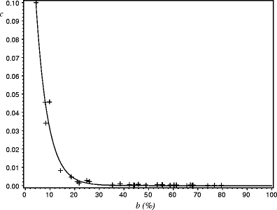
Relationship between parameters c and b provided by an individual model fitted tree by tree. Cross: observed value. Solid line: model (Eq. 8)
-
-
Third step:
The general model was re-formulated taking into account Eq. 6 and random tree and shoot effects:
-
if DTrel < CR and DSrel = 0 (i.e., for the highest branch of every shoot in the upper part of the tree)
$$ {\text{BD}} = \left( {a + {u_{\text{t}}}} \right){\text{DTrel}}\;{ \exp }\left( { - \frac{\text{DTrel}}{{\text{CR}}}} \right) + {v_{\text{ts}}} $$(9a) -
if DTrel < CR and DSrel > 0 (i.e., for all the branches situated below the highest branch of each shoot of the upper part of the tree)
$$ {\text{BD}} = \left( {\left( {a + {u_{\text{t}}}} \right){\text{DTrel}}\;{ \exp }\left( { - \frac{\text{DTrel}}{{\text{CR}}}} \right) + {v_{\text{ts}}} - d} \right){\left( {{1} - {\text{DSrel}}} \right)^f} + d $$(9b) -
if DTrel ≥ CR and DSrel = 0 (i.e., for the highest branch of every shoot in the lower part of the tree)
$$ {\text{BD}} = \left( {a + {u_{\text{t}}}} \right){\text{CR}}\;{ \exp }\left( { - {1} - c{{\left( {{\text{DTrel}} - {\text{CR}}} \right)}^{{2}}}} \right) + {v_{\text{ts}}} $$(9c) -
if DTrel ≥ CR and DSrel > 0 (i.e., for all the branches situated below the highest branch of each shoot of the lower part of the tree)
$$ {\text{BD}} = \left( {\left( {a + {u_{\text{t}}}} \right){\text{CR}}\;{ \exp }\left( { - {1} - c{{\left( {{\text{DTrel}} - {\text{CR}}} \right)}^{{2}}}} \right) + {v_{\text{ts}}} - d} \right){\left( {{1} - {\text{DSrel}}} \right)^{\text{f}}} + d $$(9d)
-
-

The relationships achieved in the second step (Eqs. 7 and 8) were included as follows:
and
where a 1, a 2, c 1, and c 2 were fixed positive parameters, common to all trees and shoots; u t and v ts were random parameters, specific to tree and annual shoots, respectively. The values estimated for the parameters are given in Table 4. The RMSE of the models are given in Table 5. Figure 2b–f shows the general model applied to sample trees.
The residuals calculated with the fixed part of the model showed no bias with the distance from the top of the tree (Fig. 4) and no effect of any tree or stand descriptor.

3.2 Branch status modeling
The probability for a branch to be alive (PBA) was significantly related to its diameter and its position inside the crown (Fig. 5). The following model accounted for the status of the branch:
where g was the logit link function and b 1, b 2, b 3, and b 4 were parameters.

Plot of branch diameter vs. insert height in a sample tree (R12 3). Dot: dead branch. Circle: living branch. The solid line shows the isoprobability for a branch to be dead or alive according to the model (Eq. 10). The horizontal dashed line represents the height of the lowest live whorl (HLW)
The predicted probabilities were transformed into a binary response (0 or 1) to compute residuals. Branches with a probability PBA < 0.5 were classified as dead and branches with a probability PBA > 0.5 were classified as living. No significant random effect was found at the tree level (i.e., the variance was estimated at 0 when the random effect was included in the model).
The curve of isoprobability for a branch to be dead or alive effectively differentiated the dead branches from the living branches (Fig. 5). Plots of residuals did not show any trend with the distance from the top of the tree (Fig. 6), nor with any tree or stand descriptor.

Mean residuals and their standard deviation from the branch death model (Eq. 10) plotted against the distance of the insert point of the branch from the top of the tree
3.3 Simulation
Figure 7 shows the simulated diameter and status of the branches of two trees. The model behavior is consistent with previous observations. The maximum branch diameter of every annual shoot increases up to the base of the living crown and then decreases up to the top of the tree. Within every annual shoot, the branch diameter clearly decreases from the top to the base of the shoot as expected. By taking into account the random shoot effect of the branch diameter model and the stochastic variability of the two models, the simulations provide realistic branch diameters and status at the tree level. Most of the branches below living crown base are dead whereas above living crown base the branches died accordingly to their diameter and position inside the crown: the thinner branches are dead higher in the living crown compared to thicker branches.

Branch diameter and branch death simulated for two trees. (a) Age: 100 years, H: 21 m, D: 25 cm. (b) Age: 100 years, H: 21 m, D: 50 cm. Only one annual shoot out of every five shoots is represented. Solid line: branch diameter model with only fixed effects. Symbols represent branch diameter simulated with additional random annual shoot and branch effects: circle: alive long shoot, dot: dead long shoot, empty triangle: alive short shoot, full triangle: dead short shoot. The line with larges dashes shows the isoprobability for a branch to be dead or alive. The vertical dotted line is for the CR value.
4 Discussion
4.1 Branch diameter model
Most published models of branch profiles have described branch dimensions using the maximum or mean branch diameter per annual shoot (e.g., Garber and Maguire 2005; Achim et al. 2006). In contrast, in this study, all the branches of each sampled annual shoot were used as individual observations. Models for pine species have obviously been developed only for whorl branches since they do not bear interwhorl branches (Mäkinen and Colin 1998; Meredieu et al. 1998). But even for forest tree species bearing interwhorl branches, the models often apply only to whorl branches (Hein et al. 2007, 2008) or to branches whose size exceeds a minimum value (Colin and Houllier 1992; Maguire et al. 1994). Moreover, when models apply to interwhorl branches, they do not use the precise position of the branches along the shoot (Hein et al. 2008), although they sometimes use the rank of the branches ordered from largest to smallest diameter (Mäkinen et al. 2003). Maguire et al. (1994) predict the maximum branch diameter in the annual shoot separately from the branch diameter expressed relative to the maximum branch diameter of the shoot as a function of relative position in the annual shoot. These two models are fitted independently from each other and provide two maximum diameter predictions which can be different, and not necessarily compatible.
The main advance of this work is to provide a new single model for individual branch diameter which accounts for both whorl and interwhorl branches. In Atlas cedar, as in Douglas fir, the distinction between whorl and interwhorl branches is rather arbitrary. Our approach reduces the pitfalls of modeling them separately.
The model form is consistent with the understanding gained on branch growth and crown development. The growth of a branch and its size depend upon both (1) its depth inside the crown, linked to growth duration or age, and (2) its position in the annual shoot because of acrotony, i.e., the predominance of the branches located at the top of the shoot. The model has a “potential x reducer” form which provides a saw-tooth profile and fits rather well the available data (Fig. 2). Equations 5a and 5c can be interpreted as a model of “potential size” which describes the thickest branch of every shoot, which is most often the highest branch in the annual shoot. From the top of the tree, the size of this branch increases downwards to a maximum value which is located near the base of the living crown (Eq. 6) and then progressively decreases to the tree bottom. The parameter a represents the slope of the model at the origin (i.e., the top of the tree). It is correlated positively with the tree diameter at breast height and the height to the base of the living crown (Eq. 7). This relationship expresses the evolution of crown shape with tree age: in old trees, the height growth stops while the diameter of stem and branches still increases. As a result, the top of the crown becomes flatter. This phenomenon is general in conifers and particularly pronounced in Cedrus genus whose mature trees are characterized by a typical flat-topped crown. Along every annual shoot, potential branch size is progressively reduced in Eqs. 5b and 5d to take into account the acrotonic gradient (Courbet et al. 2007a), i.e., the regular decrease of branch diameter downwards to the base of the shoot. Therefore, the diameter of interwhorl branches is related to their relative distance to the top of the shoot.
The model formulation ensures that the model behaves logically, i.e., the predicted value will always be positive, whereas the diameter predicted by polynomial models can theoretically have negative values (Meredieu et al. 1998). The lower limit of the branch diameter does not exceed a few millimeters because the thinnest branches die early due to lack of light penetration inside the crown as a result of self-shading among branches. The parameter d (Eq. 9b and 9d) represents the thinnest diameter to which the branch diameter tends at the base of every annual shoot. It was associated with a shoot random effect.
The highest branch was measured in every annual shoot while the diameter of all branches was measured in only one of every three annual shoots. This sample strategy results in focusing on the “potential” part of the model which describes the most important part of the crown for tree growth. On the other hand, many thinner branches were used in model fitting. Thus, the model predicts precise diameters for the type of branches which are significantly involved in wood quality.
This model does not apply to ramicorn branches which are steep angled and particularly thick. Because they rarely occur, predicting the occurrence of this type of branch certainly requires the development of a stochastic model for branch angle which takes into account the link between branch diameter and angle to the bole of the tree (e.g., Meredieu et al. 1998). This might be the object of further work based on a specific sampling strategy.
It has been widely recognized that thinning increases branch diameter, particularly the diameter of the branches situated in the lower part of the crown which is more affected by between-tree competition (Mäkinen and Hein 2006; Hein et al. 2007). Contrary to models which explicitly include stand density (Maguire et al. 1991), the effect of between-tree competition is taken into account in the model through the effect on both tree diameter at breast height and base of living crown (in Eq. 7 and position of the join point).
4.2 Branch status model
After crown closure, light interception by the canopy and mutual shading between trees limit light penetration to lower branches which causes branch death and vertical crown recession, i.e., raising the lower limit of the living crown. Whorl branch mortality is thus the result of inter-tree competition.
Branch death can also occur without between-tree competition. Mortality of thin interwhorl branches is due to within-crown competition which results in self-shading among branches in the same tree crown where the light penetration is reduced even in the crown of open-grown trees. Protz et al. (2000) considered branch mortality to be mainly driven by light limitations and to be the result of (1) lack of light energy to maintain a positive carbon balance within the branch and (2) the reduction of hydraulic permeability which is also the result of shading.
Our results show that the status of a branch is related mainly to size and vertical position, consistent with the acknowledged role of the light in branch survival. The probability of branch survival decreases with its depth into the crown and increases with its diameter and with the crown length (Eq. 10 and Table 6). Because branch diameter was included as explanatory variable in the model of branch status, it was assumed that one common model was necessary for both whorl and interwhorl branches which are only distinguishable from each other by their relative size within annual shoot. The crown length and the depth into the crown are sufficient to account for the tree and shoot effects because no significant random effects at tree and shoot levels were detected in our mixed model.
Our results are consistent with previous studies on various species which have shown the effect of branch size and vertical position on branch survival in models which included similar independent variables (e.g., Mäkinen and Colin 1999 in Scots Pine; Weiskittel et al. 2007b in Douglas fir). However, some studies have reported significant random effects (e.g., Hein et al. 2007 in Norway spruce).
The influence of stand density on branch longevity has often been reported (e.g., Hein et al. 2008). Our model accounts implicitly for this effect through the crown length. Indeed competition for light in closed stands results in vertical recession of the live crown.
4.3 Prospects
Our models, like most existing models, are static models. They assume that branch diameter profile and branch survival can be predicted from common tree measurements and stand characteristics without knowledge of stand history (Mäkinen and Colin 1998). In constrast to Mäkinen (1999), Forward and Nolan (1961) observed in tree-ring width profiles from branches located in the lower part of the living crown that thinning reactivates branch diameter growth. This may result in discontinuities in the branch diameter vertical profile at the base of the living crown and further suggests that this diameter profile may be different immediately after thinning compared to several years after thinning, all else being equal. However, in the 16 sampled trees from thinned stands we did not observe any discontinuity in the diameter vertical profiles.
Branch diameter profile and branch survival may be dynamically predicted by branch growth models fitted from increment data. However, these models are scarce because regular recording of the diameters of selected branches over a long time period in permanents plots is very time-consuming (Weiskittel et al. 2007b). It is also risky when it is necessary to climb trees (Maguire and Hann 1990). Moreover, reconstruction of past branch dimensions and status is also very difficult (Maguire and Hann 1987).
The sampling strategy used in this study was designed to cover a wide range of tree sizes and characteristics and to develop models suitable in a wide range of tree growth conditions. But our balanced sample includes only 32 trees, each one being a single representative of a particular combination of age, competitive position, site index, and stand density. Due to the small number of trees in the original sample, it was not possible to have both a calibration and a cross-validation on balanced independent subsamples. However, we expect that the validity domain of the models fitted here is sufficiently large to be applied to variously sized trees from a wide range of growth conditions. Nevertheless, it would be important to test these models on a sample independent from that used here to check the robustness of the parameters. Validation trees will have to be chosen in other stands in order to cover a range of tree size and age at least as wide as that of the calibration sample. We also expect that the model formulation is general enough to be applied to other coniferous species. It would be particularly interesting to fit our model on data from other coniferous species with interwhorl branches such as Spruces, Firs, and especially Larches, which also have long- and short-shoot axes.
The diameter and status models require knowledge of some tree and branch characteristics, in particular the height of the insertion point of the branches on the bole. We previously developed and fitted a model for Atlas cedar that describes the occurrence, the type (i.e., short shoot or long shoot) and the position of the branches along the parental shoot in a wide range of parental shoot lengths (Courbet et al. 2007a). The height of the base of the living crown is also used in both models, directly and in the crown ratio in the diameter model (Eq. 9a–9f) or in crown length in the status model (Eq. 10). This height can be easily measured. It can also be calculated from common tree descriptors (A, D, H) using an existing model available for Atlas cedar (Courbet and Houllier 2002).
These models describing branch diameter and branch status, associated with the model previously developed for branch position along the bole (Courbet et al. 2007a) can be used to predict wood quality. These traits determine the size, the type, and the position of knots which are often used in the grading rules of softwood lumber (e.g., Afnor Association française pour la normalisation 1998). In combination with models describing stem profile and internal structure (Courbet 1999; Courbet and Houllier 2002), a complete set of models is now available for the description of Atlas cedar timber quality from common tree measurements: total height and diameter at breast height.
All of these models will be associated with a tree growth model for regular and pure stands of Atlas cedar which will predict the diameter and height growth of individual trees. We have planned to implement these models in the software platform CAPSIS where a first version of the Atlas cedar growth model is already available (De Coligny et al. 2003). It will thus be possible to simulate and test easily the consequences of various silvicultural practices on growth, stem form, and branch characteristics (e.g., Fig. 7).
Our models could also be linked to process-based models which require a description of branchiness or as parameters for growth models describing the distribution of biomass or the allocation of carbon to the different compartments of the tree. This kind of model has not yet been developed specifically for Atlas cedar.
5 Conclusion
Branch size and branch status are important features which are directly related to both tree functioning and timber quality. As expected, the models developed for this study predict these two characteristics from common tree measurements (diameter at breast height, total height, and height of the base of the living crown) and branch height. These two models account for both whorl and interwhorl branches in single equations. They complete a former branch location model (Courbet et al. 2007a), thus forming a chain of consistent models useful in precise evaluation of the influence of growth on branchiness. It would be particularly interesting to fit the branch diameter model to other widespread and economically valuable coniferous species such as Spruces, Firs, and Larches.
References
Achim A, Gardiner B, Leban J-M, Daquitaine R (2006) Predicting the branching properties of Sitka spruce grown in Great Britain. N Z J For Sci 36:246–264
Afnor (Association française pour la normalisation) (1998) Règles d’utilisation du bois dans les constructions, Classement visuel pour l’emploi en structure des principales essences résineuses et feuillues, NF B 52–001, 16 p
Barthélémy D, Caraglio Y (2007) Plant architecture: a dynamic, multilevel and comprehensive approach to plant form, structure and ontogeny. Ann Bot 99:375–407
Bohrer G, Katul GG, Nathan R, Walko RL, Avissar R (2008) Effects of canopy heterogeneity, seed abscission and inertia on wind-driven dispersal kernels of tree seeds. J Ecol 96:569–580
Colin F, Houllier F (1991) Branchiness of Norway spruce in north-eastern France: modelling vertical trends in maximum nodal branch size. Ann Sci For 48:679–693
Colin F, Houllier F (1992) Branchiness of Norway spruce in northeastern France: predicting the main crown characteristics from usual tree measurements. Ann Sci For 49:511–538
Courbet F (1999) A three-segmented model for the vertical distribution of annual ring area. Application to Cedrus atlantica Manetti. For Ecol Manag 119:177–194
Courbet F, Houllier F (2002) Modelling the profile and internal structure of tree stem. Application to Cedrus atlantica (Manetti). Ann Sci For 59:63–80
Courbet F, Sabatier S, Guédon Y (2007a) Predicting the vertical location of branches along Atlas cedar stem (Cedrus atlantica Manetti) in relation to annual shoot length. Ann For Sci 64:707–718
Courbet F, Courdier J-M, Mariotte N, Courdier F (2007b) Croissance, production et conduite des peuplements de cèdre de l’Atlas. Forêt Entreprise 174:40–44
De Coligny F, Ancelin P, Cornu G, Courbaud B, Dreyfus P, Goreaud F, Gourlet-Fleury S, Meredieu C, Saint-André L (2003) CAPSIS: Computer-Aided Projection for Strategies in Silviculture: advantages of a shared forest-modelling platform. In: Amaro A, Reed D, Soares P (eds) Modelling Forest Systems. CABI Publishing, UK, pp 319–323
Doruska PF, Burkhart HE (1994) Modeling the diameter and locational distribution of branches within the crowns of loblolly pine trees in unthinned plantations. Can J For Res 24:2362–2376
Evans M-A (1996) Etude et modélisation de la croissance en hauteur dominante du Cèdre de l’Atlas en région méditerranéenne. Technical report, Institut National Agronomique Paris-Grignon, 21 p
Forward DF, Nolan NJ (1961) Growth and morphogenesis in the Canadian forest species. IV. Radial growth in branches and main axis of Pinus resinosa Ait. under conditions of open growth, suppression and release. Can J Bot 39:385–409
Garber SM, Maguire DA (2005) Vertical trends in maximum branch diameter in two mixed-species spacing trials in the central Oregon Cascades. Can J For Res 35:295–307
Hein S, Mäkinen H, Yue C, Kohnle U (2007) Modelling branch characteristics of Norway spruce from wide spacing in Germany. For Ecol Manag 242:155–164
Hein S, Weiskittel AR, Kohnle U (2008) Branch characteristics of widely spaced Douglas-fir in south-western Germany: comparisons of modelling approaches and geographic regions. For Ecol Manag 256:1064–1079
Letort V, Cournède P-H, Mathieu A, de Reffye P, Constant T (2008) Parametric identification of a functional-structural tree growth model and application to beech trees (Fagus sylvatica). Funct Plant Biol 35:951–963
Littell RC, Milliken GA, Stroup WW, Wolfinger RD (1996) SAS® system for mixed models. SAS Institute Inc., Cary, 633 p
Maguire DA, Hann DW (1987) A Stem Dissection Technique for Dating Branch Mortality and Reconstructing Past Crown Recession. For Sci 33:858–871
Maguire DA, Hann DW (1990) A Sampling Strategy for Estimating Past Crown Recession on Temporary Growth Plots. For Sci 36:549–563
Maguire DA, Kershaw JA, Hann DW (1991) Predicting the effects of silvicultural regime on branch size and crown wood core in Douglas-fir. For Sci 37:1409–1428
Maguire DA, Moeur M, Bennett WS (1994) Models for describing basal diameter and vertical distribution of primary branches in young Douglas-fir. For Ecol Manag 63:23–55
Mäkelä A (2002) Derivation of stem taper from the pipe model theory in a carbon balance framework. Tree Physiol 22:891–905
Mäkinen H (1999) Effect of stand density on radial growth of branches of Scots pine in southern and central Finland. Can J For Res 29:1216–1224
Mäkinen H, Colin F (1998) Predicting branch angle and branch diameter of Scots pine from usual tree measurements and stand structural information. Can J For Res 28:1686–1696
Mäkinen H, Colin F (1999) Predicting the number, death, and self pruning of branches in Scots pine. Can J For Res 29:1225–1236
Mäkinen H, Hein S (2006) Effect of wide spacing on increment and branch properties of young Norway spruce. Eur J For Res 125:239–248
Mäkinen H, Ojansuu R, Sairenen P, Yli-Kojola H (2003) Predicting branch characteristics of Norway spruce (Picea abies (L.) Karst.). Forestry 76:525–546
Meredieu C, Colin F, Hervé J-C (1998) Modelling branchiness of Corsican pine with mixed-effect models (Pinus nigra Arnold ssp. laricio (Poiret) Maire). Ann For Sci 55:359–374
Perttunen J, Sievänen R, Nikinmaa E (1998) LIGNUM: a model combining the structure and the functioning of trees. Ecol Model 108:189–198
Protz CG, Silins U, Lieffers VJ (2000) Reduction in branch sapwood hydraulic permeability as a factor limiting survival of lower branches of lodgepole pine. Can J For Res 30:1088–1095
Rigolot R, de Coligny F, Dreyfus Ph, Dupuy J-L, Lecomte I, Pezzatti B, Vigy O, Pimont F (2010) In: Viegas DX (ed) Fuel Manager: a vegetation assessment and manipulation software for wildfire modelling. Proceedings of the 6th International Conference on Forest Fire Research. University of Coimbra, Portugal, p 12
Riou-Nivert Ph (2007) Climat propice pour le cèdre. Forêt Entreprise 174:12–13
Roeh RL, Maguire DA (1997) Crown profile models based on branch attributes in coastal Douglas-fir. For Ecol Manag 96:77–100
Sabatier S, Barthélémy D (1999) Growth dynamics and morphology of annual shoots, according to their architectural position, in young Cedrus atlantica (Endl.) Manetti ex. Carrière (Pinaceae). Ann Bot 84:387–392
SAS Institute Inc. (2000) SAS/STAT® User’s Guide, Version 8. SAS Institute Inc, Cary, p 3809
Torodoki CL, Monserud RA, Parry DL (2005) Predicting internal lumber grade from log surface knots; actual and simulated results. For Prod J 55:38–47
Weiskittel AR, Maguire DA, Monserud RA (2007a) Modeling crown structural responses to competing vegetation control, thinning, fertilization, and Swiss needle cast in coastal Douglas-fir of the Pacific Northwest, USA. For Ecol Manag 245:96–109
Weiskittel AR, Maguire DA, Monserud RA (2007b) Response of branch growth and mortality to silvicultural treatments in coastal Douglas-fir plantations: Implications for predicting tree growth. For Ecol Manag 251:182–194
Acknowledgements
This work was partially supported by a grant from the French Ministry of Agriculture (DERF Convention 61.45.34/00). We are grateful to Anne Albouy, Jacques-Olivier Fouasse, Nicolas Mariotte, and Olivier Richer for technical and field assistance and to the National Forest Service (ONF) for providing the sample trees. We thank Tonya Lander for language review and improvement and François Pimont for constructive suggestions.
Open Access
This article is distributed under the terms of the Creative Commons Attribution Noncommercial License which permits any noncommercial use, distribution, and reproduction in any medium, provided the original author(s) and source are credited.
Author information
Authors and Affiliations
Corresponding author
Additional information
Handling Editor: Gérard Nepveu
Rights and permissions
Open Access This is an open access article distributed under the terms of the Creative Commons Attribution Noncommercial License (https://creativecommons.org/licenses/by-nc/2.0), which permits any noncommercial use, distribution, and reproduction in any medium, provided the original author(s) and source are credited.
About this article
Cite this article
Courbet, F., Hervé, JC., Klein, E.K. et al. Diameter and death of whorl and interwhorl branches in Atlas cedar (Cedrus atlantica Manetti): a model accounting for acrotony. Annals of Forest Science 69, 125–138 (2012). https://doi.org/10.1007/s13595-011-0156-1
Received:
Accepted:
Published:
Issue Date:
DOI: https://doi.org/10.1007/s13595-011-0156-1