On finite dimensional Nichols algebras of diagonal type

Alles Gescheidte ist schon gedacht worden, man muß nur versuchen es noch einmal zu denken.

Goethe

Abstract

This is a survey on Nichols algebras of diagonal type with finite dimension, or more generally with arithmetic root system. The knowledge of these algebras is the cornerstone of the classification program of pointed Hopf algebras with finite dimension, or finite Gelfand–Kirillov dimension; and their structure should be indispensable for the understanding of the representation theory, the computation of the various cohomologies, and many other aspects of finite dimensional pointed Hopf algebras. These Nichols algebras were classified in Heckenberger (Adv Math 220:59–124, 2009) as a notable application of the notions of Weyl groupoid and generalized root system (Heckenberger in Invent Math 164:175–188, 2006; Heckenberger and Yamane in Math Z 259:255–276, 2008). In the first part of this monograph, we give an overview of the theory of Nichols algebras of diagonal type. This includes a discussion of the notion of generalized root system and its appearance in the contexts of Nichols algebras of diagonal type and (modular) Lie superalgebras. In the second and third part, we describe for each Nichols algebra in the list of Heckenberger (2009) the following basic information: the generalized root system; its label in terms of Lie theory; the defining relations found in Angiono (J Eur Math Soc 17:2643–2671, 2015; J Reine Angew Math 683:189–251, 2013); the PBW-basis; the dimension or the Gelfand–Kirillov dimension; the associated Lie algebra as in Andruskiewitsch et al. (Bull Belg Math Soc Simon Stevin 24(1):15–34, 2017). Indeed the second part deals with Nichols algebras related to Lie algebras and superalgebras in arbitrary characteristic, while the third contains the information on Nichols algebras related to Lie algebras and superalgebras only in small characteristic, and the few examples yet unidentified in terms of Lie theory.

1 Introduction

1.1 What is a Nichols algebra?

1. Let $\mathbb {k}$ be a field, V a vector space and $c \in GL (V \otimes V)$. The braid equation on c is

$$\begin{aligned} (c\otimes {\text {id}})({\text {id}}\otimes c)(c\otimes {\text {id}}) = ({\text {id}}\otimes c)(c\otimes {\text {id}})({\text {id}}\otimes c). \end{aligned}$$

(0.1)

If c satisfies (0.1), then the pair (V, c) is a braided vector space. The braid equation, or the closely related quantum Yang–Baxter equation, is the key to many developments in the last 50 years in several areas in mathematics and theoretical physics. Ultimately these applications come from the representations $\varrho _n$ of the braid groups $\mathbb {B}_n$ on $T^n(V)$ induced by (0.1), for $n \ge 2$. Indeed, let $\mathbb {I}_{n} := \{1, 2, \ldots , n\}$, where n is a natural number. Recall that $\mathbb {B}_n$ is presented by generators $(\sigma _j)_{j \in \mathbb {I}_{n-1}}$ with relations

$$\begin{aligned} \sigma _j \sigma _k = \sigma _k\sigma _j,\quad \vert j-k \vert \ge 2, \quad \sigma _j \sigma _k\sigma _j = \sigma _k\sigma _j\sigma _k,\quad \vert j-k \vert = 1. \end{aligned}$$

(0.2)

Thus $\varrho _n$ applies $\sigma _j \mapsto {\text {id}}_{V^{\otimes (j-1)}} \otimes c \otimes {\text {id}}_{V^{\otimes (n - j-1)}}$.

2. Assume that $\mathrm{char}\,\mathbb {k}\ne 2$. Let c be a symmetry, i.e. a solution of (0.1) such that $c^2 = {\text {id}}$. Then $\varrho _n$ factorizes through the representation $\widetilde{\varrho }_n$ of the symmetric group $\mathbb {S}_n$ given by $s_j := (j \, j+1) \mapsto {\text {id}}_{V^{\otimes (j-1)}} \otimes c \otimes {\text {id}}_{V^{\otimes (n - j-1)}}$. The symmetric algebra of (V, c) is the quadratic algebra

$$\begin{aligned} S_c(V) = T(V)/ \langle \ker (c + {\text {id}}) \rangle = \oplus _{n\in \mathbb {N}_0} S^n_c(V). \end{aligned}$$

For instance, if $c = \tau$ is the usual transposition, then $S_c(V) = S(V)$, the classical symmetric algebra; while if $V = V_0 \oplus V_1$ is a super vector space and c is the super transposition, then $S_c(V) \simeq S(V_0) \underline{\otimes } \Lambda (V_1)$, the super symmetric algebra.

The adequate setting for such symmetries is that of symmetric tensor categories, advocated by Mac Lane in 1963. In this context, the symmetric algebra satisfies the same universal property as in the classical definition. In particular, symmetric algebras are Hopf algebras in symmetric tensor categories. Assume that $\mathrm{char}\,\mathbb {k}= 0$. Then, as vector spaces,

$$\begin{aligned} S^n_c(V) \simeq T^n(V)^{\mathbb {S}_n} = {\text {Im}}\textstyle \int _n \simeq T^n(V) / \ker \int _n, \end{aligned}$$

(0.3)

where $\int _n = \sum _{s \in \mathbb {S}_n} \widetilde{\varrho }_n(s){:}\,T^n(V) \rightarrow T^n(V)$.

3. The adequate setting for braided vector spaces is that of braided tensor categories [56]; there is a natural notion of Hopf algebra in such categories.

Let H be a Hopf algebra (with bijective antipode). Then H gives rise to a braided tensor category ${}^{H}_{H}\mathcal {YD}$ [39], and consequently is a source of examples of braided vector spaces. Namely, an object $M \in {}^{H}_{H}\mathcal {YD}$, called a Yetter–Drinfeld module over H, is simultaneously a left H-module and a left H-comodule satisfying the compatibility condition

$$\begin{aligned} \delta (h \cdot v) = h_{\left( 1 \right) }v_{\left( -1 \right) } \mathcal {S}(h_{\left( 3 \right) }) \otimes h_{\left( 2 \right) } \cdot v_{\left( 0 \right) },\quad h\in H, \, v\in V. \end{aligned}$$

(0.4)

This is a braided tensor category with the usual tensor product of modules and comodules, and braiding

$$\begin{aligned} c_{M, N}(x\otimes y) = x_{\left( -1 \right) } \cdot y \otimes x_{\left( 0 \right) },\quad M, N \in {}^{H}_{H}\mathcal {YD},\, x\in M,\, y\in N. \end{aligned}$$

(0.5)

For $M \in {}^{H}_{H}\mathcal {YD}$, $c = c_{M, M} \in GL (M \otimes M)$ satisfies the braid equation (0.1).

If $M \in {}^{H}_{H}\mathcal {YD}$, then the tensor algebra T(M) is a Hopf algebra in ${}^{H}_{H}\mathcal {YD}$, whose coproduct is determined by $\Delta (x) = x \otimes 1 + 1 \otimes x$ for $x \in M$. Also the tensor coalgebra $T^c(M)$ is a Hopf algebra in ${}^{H}_{H}\mathcal {YD}$, with braided shuffle product. See [76, Proposition 9].

4. Let (V, c) be a braided vector space but c not necessarily a symmetry. The Nichols algebra ${\mathcal {B}}(V) = \oplus _{n\in \mathbb {N}_0} {\mathcal {B}}^n (V)$ of (V, c) is a graded connected algebra with a number of remarkable properties that has at least superficially a resemblance with a symmetric algebra.¹ For, let $M_n{:}\,\mathbb {S}_n \rightarrow \mathbb {B}_n$ be the (set-theoretical) Matsumoto section, that preserves the length and satisfies $M_n(s_j) = \sigma _j$. Let $\Omega _n = \sum _{\sigma \in \mathbb {S}_n} \varrho _n (M_n(\sigma ))$ and ${\mathcal {J}}^n(V) = \ker \Omega _n$. Define

$$\begin{aligned} {\mathcal {J}}(V) = \oplus _{n\ge 2}{\mathcal {J}}^n(V),\quad {\mathcal {B}}(V) = T(V){/}{\mathcal {J}}(V). \end{aligned}$$

(0.6)

Despite the similarity of (0.3) and (0.6), Nichols algebras have profound divergences with symmetric algebras—and various analogies.

• (a) The subspace ${\mathcal {J}}(V)$ is actually a two-sided ideal of T(V), so that ${\mathcal {B}}(V)$ is a connected graded algebra generated in degree 1. However ${\mathcal {J}}(V)$ is seldom quadratic, and it might well be not finitely generated. The determination of ${\mathcal {J}}(V)$ is one of the central problems of the subject.

• (b) Although (0.6) is a compact definition, it hides the rich structure of Nichols algebras. Indeed, ${\mathcal {B}}(V)$ is a Hopf algebra in ${}^{H}_{H}\mathcal {YD}$ for suitable H. Even more, it is a coradically graded coalgebra, a notion dual to generation in degree one.

• (c) If V is a finite-dimensional vector space, then $S(V^*)$ is identified with the algebra of differential operators on S(V) (with constant coefficients). An analogous description is available for Nichols algebras, being useful to find relations of ${\mathcal {B}}(V)$.

• (d) Nichols algebras appeared in various fronts. In [71], they were defined for the first time as a tool to construct new examples of Hopf algebras. They are instrumental for the attempt in [86] to define a non-commutative differential calculus on Hopf algebras. Also, the positive part $U^+_q(\mathfrak {g})$ of the quantized enveloping algebra of a Kac–Moody algebra $\mathfrak {g}$ at a generic parameter q turns out to be a Nichols algebra [67, 75, 78].

By various reasons, we are also led to consider:

• Pre-Nichols algebras of the braided vector space (V, c) [26, 69]; these are graded connected Hopf algebras in ${}^{H}_{H}\mathcal {YD}$, say ${\mathcal {B}}= \oplus _{n\in \mathbb {N}_0} {\mathcal {B}}^n$, with ${\mathcal {B}}^1 \simeq V$, that are generated in degree 1 (but not necessarily coradically graded). Thus we have epimorphisms of Hopf algebras in ${}^{H}_{H}\mathcal {YD}$

  

• Post-Nichols algebras of the braided vector space (V, c) [7]; these are graded connected Hopf algebras in ${}^{H}_{H}\mathcal {YD}$, say ${\mathcal {E}}= \oplus _{n\in \mathbb {N}_0} {\mathcal {E}}^n$, with ${\mathcal {E}}^1 \simeq V$, that are coradically graded (but not necessarily generated in degree 1). Thus we have monomorphisms of Hopf algebras in ${}^{H}_{H}\mathcal {YD}$

  

Thus, the only pre-Nichols algebra that is also post-Nichols is ${\mathcal {B}}(V)$ itself.

1.2 Classes of Nichols algebras

5. Nichols algebras are basic invariants of Hopf algebras that are not generated by its coradical [11, 18]; see the discussion in Sect. 1.7. One is naturally led to the following questions.

1.2.1 Classify all $V \in {}^{H}_{H}\mathcal {YD}$ such that the (Gelfand–Kirillov) dimension of ${\mathcal {B}}(V)$ is finite. For such V, determine the generators of the ideal ${\mathcal {J}}(V)$ and all post-Nichols algebras ${\mathcal {B}}(V) \hookrightarrow {\mathcal {E}}$ with finite (Gelfand–Kirillov) dimension

Now ${\mathcal {B}}(V)$ is a Hopf algebra in ${}^{H}_{H}\mathcal {YD}$ but the underlying algebra depends only on the braiding c, and reciprocally the same braided vector space can be realized in ${}^{H}_{H}\mathcal {YD}$ in many ways and for many H’s. That is, we may deal with the above problems for suitable classes of braided vector spaces.

Also, assume that (V, c) satisfies, for some $\theta \in \mathbb {N}_{>1}$,

$$\begin{aligned} V = V_{1} \oplus \cdots \oplus V_\theta ,\quad c(V_i \otimes V_j) = V_j \otimes V_i,\quad i,j\in \mathbb {I}_{\theta }. \end{aligned}$$

(0.7)

So, we may suppose that the ${\mathcal {B}}(V_i)$’s are known and try to infer the shape of ${\mathcal {B}}(V)$ from them and the cross-braidings $c_{\vert V_i \otimes V_j}$; this viewpoint leads to a rich combinatorial analysis [5, 16, 44, 48, 50, 52].

6. The simplest yet most fundamental examples are those (V, c) satisfying (0.7) with $\dim V_i = 1$, $i\in \mathbb {I}= \mathbb {I}_{\theta }$. Pick $x_i \in V_i - 0$; then $(x_i)_{i\in \mathbb {I}}$ is a basis of V, and $c(x_i\otimes x_j)=q_{ij}\, x_j\otimes x_i$, $i,j\in \mathbb {I}$, where $q_{ij} \in \mathbb {k}^{\times }$. We say that (V, c) is a braided vector space of diagonal type if

$$\begin{aligned} q_{ii} \ne 1,\quad \text {for all } i \in \mathbb {I}. \end{aligned}$$

Notice that this condition, assumed by technical reasons, is not always required in the literature. See [5, Lemma 2.8].

This class appears naturally when $H = \mathbb {k}\Gamma$, where $\Gamma$ is an abelian group, but also lays behind any attempt to argue inductively. Other classes of braided vector spaces were considered in the literature:

• (a) Triangular type, see [5, 84].

• (b) Rack type, arising from non-abelian groups, see references in [1].

• (c) Semisimple (but not simple) Yetter–Drinfeld modules [5, 48,49,50], and references therein.

• (d) Yetter–Drinfeld modules over Hopf algebras that are not group algebras, see for example [4, 13, 14, 43, 54, 55].

1.3 Nichols algebras of diagonal type

7. Assume now that $\mathbb {k}$ is algebraically closed and of characteristic 0. The classification of the braided vector spaces (V, c) of diagonal type with finite-dimensional ${\mathcal {B}}(V)$ was obtained in [46]. (When $\mathrm{char}\,\mathbb {k}> 0$, the classification is known under the hypothesis $\dim V \le 3$ [51, 85]). The core of the approach is the notion of generalized root system; actually, the paper [46] contains the list of all (V, c) of diagonal type with connected Dynkin diagram and finite generalized root system (these are called arithmetic). The list can be roughly split in several classes:

• Standard type [2], that includes Cartan type [19]; related to the Lie algebras in the Killing–Cartan classification.

• Super type [10], related to the finite-dimensional contragredient Lie superalgebras in characteristic 0, classified in [57].

• Modular type [3], related to the finite-dimensional contragredient Lie (super)algebras in positive characteristic, classified in [29, 59].

• A short list of examples not (yet) related to Lie theory, baptised UFO’s.

The goal of this work is to give exhaustive information on the structure of these Nichols algebras.

8. This monograph has three Parts. Part I is an exposition of the basics of Nichols algebras of diagonal type. Section 1 is a potpourri of various topics needed for further discussions. The bulk of this Part is Sect. 2 where the main notions that we display later are explained: PBW-basis, generalized root systems, and so on. In Parts II and III we give the list of all finite-dimensional Nichols algebra of diagonal type (with connected Dynkin diagram) classified in [46] and for each of them, its fundamental information. For more details see Sect. 3, p. 47.

Part I. General facts

2 Preliminaries

2.1 Notation

In this paper, $\mathbb {N}= \{1, 2, 3, \ldots \}$ and $\mathbb {N}_0 = \mathbb {N}\cup \{0\}$. If $k < \theta \in \mathbb {N}_0$, then we denote $\mathbb {I}_{k, \theta } = \{n\in \mathbb {N}_0{:}\,k\le n \le \theta \}$. Thus $\mathbb {I}_{\theta } = \mathbb {I}_{1, \theta }$.

The base field $\mathbb {k}$ is algebraically closed of characteristic zero (unless explicitly stated); we set $\mathbb {k}^{\times } = \mathbb {k}- 0$. All algebras will be considered over $\mathbb {k}$. If R is an algebra and $J\subset R$, we will denote by $\langle J\rangle$ the 2-sided ideal generated by J and by $\mathbb {k}\langle J\rangle$ the subalgebra generated by J, or $\mathbb {k}[J]$ if R is commutative. Also ${\text {Alg}}(R,\mathbb {k})$ denotes the set of algebra maps from R to $\mathbb {k}$.

For each integer $N>1$, $\mathbb {G}_N$ denotes the group of Nth roots of unity in $\mathbb {k}$, and $\mathbb {G}'_N$ is the corresponding subset of primitive roots (of order N). Also $\mathbb {G}_{\infty } = \bigcup _{N \in \mathbb {N}} \mathbb {G}_N$, $\mathbb {G}'_{\infty } =\mathbb {G}_{\infty } - \{1\}$. We will denote by $\Gamma$ an abelian group and by $\widehat{\Gamma }$ the group of characters of $\Gamma$.

We shall use the notation for q-factorial numbers: for $q\in \mathbb {k}^\times$, $n\in \mathbb {N}$,

$$\begin{aligned} (0)_q! =1,\quad (n)_q=1+q+\cdots +q^{n-1},\quad (n)_q!=(1)_q(2)_q\ldots (n)_q. \end{aligned}$$

2.2 Kac–Moody algebras

Recall from [58] that $A = (a_{ij})\in \mathbb {Z}^{\theta \times \theta }$ is a generalized Cartan matrix (GCM) if for all $i, j \in \mathbb {I}$

$$\begin{aligned} a_{ii} = 2, \quad a_{ij} \le 0, \ i\ne j,\quad a_{ij} = 0 \iff a_{ji} =0. \end{aligned}$$

(1.1)

It is equivalent to give Cartan matrix or to give a Dynkin diagram, cf. [58]. Also, A is indecomposable if its Dynkin diagram is connected, see [58]; and is symmetrizable if there exists a diagonal matrix D such that DA is symmetric. Indecomposable and symmetrizable GCM’s fall into one of three classes:

• (a) Finite; those whose corresponding Kac–Moody algebra has finite dimension, i.e. those in Killing–Cartan classification.

• (b) Affine; those whose corresponding Kac–Moody algebra has infinite dimension but is of polynomial growth.

• (c) Indefinite; the rest.

Let A be a GCM. We denote by $\mathfrak {g}(A)$ the corresponding Kac–Moody algebra, see [58] and Sect. 2.8 below. Also $\varDelta ^A_+$ denotes the set of positive roots, so that $\varDelta ^A = \varDelta ^A_+ \cup -\varDelta ^A_+$ is the set of all roots. Further, $\varDelta ^{A, \text {re}}_+$, $\varDelta ^{A, \text {im}}_+$, are the sets of positive real, respectively imaginary, roots.

2.3 Hopf algebras

We use standard notation for coalgebras and Hopf algebras: the coproduct is denoted by $\Delta$, the counit by $\varepsilon$ and the antipode by $\mathcal {S}$. For the first we use the Heyneman–Sweedler notation $\Delta (x)=\sum x_{(1)}\otimes x_{(2)}$; the summation sign will be often omitted. All Hopf algebras are supposed to have bijective antipode; the composition inverse of $\mathcal {S}$ is denoted by $\overline{\mathcal {S}}$. Let H be a Hopf algebra. We denote by G(H) the set of group-like elements of H. The tensor category of finite-dimensional representations of H is denoted $\mathrm{Rep}\,H$. If the group of group-likes $G(H)=\Gamma$ is abelian, $g\in \Gamma$ and $\chi \in \widehat{\Gamma }$, then $\mathcal {P}_{(1,g)}^\chi (H)$ denotes the isotypical component of type $\chi$ of the space of (1, g)-primitive elements.

For more information on Hopf algebras see [70, 73].

2.4 Yetter–Drinfeld modules

The definition of these was given in Sect. 3 of the Introduction.

As in every monoidal category, there are algebras and coalgebras in ${}^{H}_{H}\mathcal {YD}$:

• $(A, \mu )$ is an algebra in ${}^{H}_{H}\mathcal {YD}$ means that A is an object in ${}^{H}_{H}\mathcal {YD}$ that bears an associative unital multiplication $\mu$ such that $\mu {:}\,A \otimes A \rightarrow A$ and the unit $u{:}\,\mathbb {k}\rightarrow A$ are morphisms in ${}^{H}_{H}\mathcal {YD}$.

• $(C, \Delta )$ is a coalgebra in ${}^{H}_{H}\mathcal {YD}$ means that C is an object in ${}^{H}_{H}\mathcal {YD}$ that bears a coassociative counital comultiplication $\Delta$ such that $\Delta {:}\,C \rightarrow C \otimes C$ and the counit $\varepsilon {:}\,C\rightarrow \mathbb {k}$ are morphisms in ${}^{H}_{H}\mathcal {YD}$.

The category of algebras in ${}^{H}_{H}\mathcal {YD}$ is again monoidal; if $(A, \mu _A)$, $(B, \mu _B)$ are algebras in ${}^{H}_{H}\mathcal {YD}$, then $A \underline{\otimes } B := (A \otimes B, \mu _{A \otimes B})$ also is, where

$$\begin{aligned} \mu _{A \otimes B} = (\mu _{A} \otimes \mu _{B}) ({\text {id}}_A \otimes c_{B, A} \otimes {\text {id}}_B). \end{aligned}$$

(1.2)

Analogously, if $(C, \Delta _C)$, $(D, \Delta _D)$ are coalgebras in ${}^{H}_{H}\mathcal {YD}$, then $C \underline{\otimes } D := (C \otimes D, \Delta _{C \otimes D})$ also is, where

$$\begin{aligned} \Delta _{C \otimes D} = ({\text {id}}_C \otimes c_{C, D} \otimes {\text {id}}_D) (\Delta _{C} \otimes \Delta _{D}). \end{aligned}$$

(1.3)

We are mainly interested in the case $H=\mathbb {k}\Gamma$, where $\Gamma$ is an abelian group; a Yetter–Drinfeld module over $\mathbb {k}\Gamma$ is a $\Gamma$-graded vector space $M =\bigoplus _{t\in \Gamma }M_t$ provided with a linear action of $\Gamma$ such that

$$\begin{aligned} t\cdot M_h = M_{h},\quad t,h\in \Gamma . \end{aligned}$$

(1.4)

Here (1.4) is just (0.4) in this setting. Morphisms in ${}^{\mathbb {k}\Gamma }_{\mathbb {k}\Gamma }\mathcal {YD}$ are linear maps preserving the action and the grading. Let $M\in {}^{\mathbb {k}\Gamma }_{\mathbb {k}\Gamma }\mathcal {YD}$. Then we set

$$\begin{aligned} M^{\chi }_t = \left\{ v\in M_t{:}\,h\cdot v=\chi (h)v, \forall h\in \Gamma \right\} ,\quad t\in \Gamma , \, \chi \in \widehat{\Gamma }. \end{aligned}$$

The braiding $c_{M, N}{:}\,M\otimes N\rightarrow N\otimes M$, cf. (0.1), is given by

$$\begin{aligned} c_{M, N}(x\otimes y) = t \cdot y \otimes x, \quad x\in M_t,\, t\in \Gamma ,\, y\in N. \end{aligned}$$

(1.5)

2.5 Braided Hopf algebras

Since it is a braided monoidal category, there are also Hopf algebras in ${}^{H}_{H}\mathcal {YD}$. Let us describe them explicitly when $H = \mathbb {k}\Gamma$, $\Gamma$ an abelian group, for illustration. A Hopf algebra in ${}^{\mathbb {k}\Gamma }_{\mathbb {k}\Gamma }\mathcal {YD}$ is a collection $(R, \mu , \Delta )$, where

• $R\in {}^{\mathbb {k}\Gamma }_{\mathbb {k}\Gamma }\mathcal {YD}$;

• $(R, \mu )$ is an algebra in ${}^{\mathbb {k}\Gamma }_{\mathbb {k}\Gamma }\mathcal {YD}$ and $(R, \Delta )$ is a coalgebra in ${}^{\mathbb {k}\Gamma }_{\mathbb {k}\Gamma }\mathcal {YD}$;

• $\Delta {:}\,R \rightarrow R \underline{\otimes } R$ and $\varepsilon {:}\,R \rightarrow \mathbb {k}$ are algebra maps;

• R has an antipode $\mathcal {S}_R$, i.e. a convolution inverse of the identity of R.

Let R be a Hopf algebra in ${}^{\mathbb {k}\Gamma }_{\mathbb {k}\Gamma }\mathcal {YD}$. Then $R\#\mathbb {k}\Gamma = R\otimes \mathbb {k}\Gamma$ with the smash product algebra and smash coproduct coalgebra structures is a Hopf algebra, called the bosonization of R by $\mathbb {k}\Gamma$, see [68, Theorem 6.2.2].

The adjoint representation ${\text {ad}}_c{:}\,R\rightarrow \mathrm{End}\,R$ is the linear map given by

$$\begin{aligned} {\text {ad}}_c x(y) = \mu (\mu \otimes \mathcal S)({\text {id}}\otimes c)(\Delta \otimes {\text {id}})(x\otimes y),\quad x,y\in R. \end{aligned}$$

(1.6)

It can be shown that ${\text {ad}}_c x(y) = {\text {ad}}x(y)$, $x,y \in R$, where ad is the adjoint representation of $R\#\mathbb {k}\Gamma$.

2.6 Nichols algebras

We are now ready to discuss the central notion of this monograph. At the beginning we place ourselves in the context of a general Hopf algebra H with bijective antipode, although for the later discussion from Sect. 2 on, $H = \mathbb {k}\Gamma$, $\Gamma$ an abelian group, is general enough.

Let $V \in {}^{H}_{H}\mathcal {YD}$. Clearly the tensor algebra T(V) and the tensor coalgebra $T^c(V)$ are objects in ${}^{H}_{H}\mathcal {YD}$. Then:

• There is an algebra map $\Delta {:}\,T(V) \rightarrow T(V) \underline{\otimes } T(V)$ determined by

  $$\begin{aligned} \Delta (v) = v \otimes 1 + 1 \otimes v,\quad v\in V; \end{aligned}$$

  with this, T(V) is a graded Hopf algebra in ${}^{H}_{H}\mathcal {YD}$.

• There is a coalgebra map $\mu {:}\,T^c(V) \underline{\otimes } T^c(V) \rightarrow T^c(V)$ determined by

  $$\begin{aligned} \mu (v \otimes 1) = v = \mu (1 \otimes v),\quad v\in V; \end{aligned}$$

  with this, $T^c(V)$ is a graded Hopf algebra in ${}^{H}_{H}\mathcal {YD}$ [76, Proposition 9].

• There is a morphism $\Omega {:}\,T(V) \rightarrow T^c(V)$ of graded Hopf algebras in ${}^{H}_{H}\mathcal {YD}$ such that $\Omega _{|V} = {\text {id}}_V$. We denote $\Omega _n= \Omega _{| T^n(V)}$, so that $\Omega = \sum _n \Omega _n$.

Definition 1.1

The Nichols algebra ${\mathcal {B}}(V)$ is the quotient of the tensor algebra T(V) by the ideal ${\mathcal {J}}(V) := \ker \Omega$, which is (isomorphic to) the image of the map $\Omega$. Thus, ${\mathcal {J}}(V) = \oplus _{n \ge 2} {\mathcal {J}}^n(V)$, where ${\mathcal {J}}^n(V) = \ker \Omega _n$.

Nichols algebras play a fundamental role in the classification of pointed Hopf algebras, see [20] and Sect. 1.7 below. As algebras or coalgebras, their structure depends only on the braided vector space (V, c) and not on the realization in ${}^{H}_{H}\mathcal {YD}$, cf. Proposition 1.2(a). We now state various alternative descriptions of ${\mathcal {B}}(V)$, or more precisely of the ideal ${\mathcal {J}}(V) = \oplus _{n\ge 2} {\mathcal {J}}^n(V)$. To start with we introduce the left and right skew derivations. See e.g. [16] for more details. Let $f \in V^*$. Let $\partial ^L_{f} = \widetilde{\partial }_{f} \in \mathrm{End}\,T(V)$ be given by

$$\begin{aligned} \widetilde{\partial }_f(1)&=0,&\widetilde{\partial }_f(v) = f(v), \forall v\in V, \end{aligned}$$

(1.7)

$$\begin{aligned} \widetilde{\partial }_f(xy)&= \widetilde{\partial }_f(x)y + \sum _i x_i \widetilde{\partial }_{f_i}(y),&\text {where } c^{-1} (f \otimes x) = \sum _i x_i \otimes f_i. \end{aligned}$$

(1.8)

Analogously, let $\partial ^R_{f} = \partial _{f}\in \mathrm{End}\,T(V)$ be given by (1.7) and

$$\begin{aligned} \partial _f(xy) = x\partial _f(y) + \sum _j \partial _{f_j}(x) y_j,\quad \text {where } c^{-1} (y \otimes f) = \sum _j f_j \otimes y_j. \end{aligned}$$

(1.9)

Let us fix a basis $(x_i)_{i\in \mathbb {I}}$ of V and let $(f_i)_{i\in \mathbb {I}}$ be its dual basis; set $\partial _i = \partial _{f_i}$, $\widetilde{\partial }_i = \widetilde{\partial }_{f_i}$, $i\in \mathbb {I}$. There is a particular instance where (1.9) has a simpler expression: assume that there exists a family $(g_i)_{i\in \mathbb {I}}$ in G(H) such that $\delta (x_i) = g_i \otimes x_i$, for every $i \in \mathbb {I}$. Then (1.9) for all f is equivalent to

$$\begin{aligned} \partial _i(xy) = x\partial _i(y) + \partial _i(x) \,g_i\cdot y,\quad x,y\in T(V),\quad i\in \mathbb {I}. \end{aligned}$$

(1.10)

Recall the Matsumoto section $M_n{:}\,\mathbb {S}_n \rightarrow \mathbb {B}_n$, cf. Sect. 4 of the Introduction. Here are the promised alternative descriptions.

Proposition 1.2

• (a) $\Omega _n = \sum _{\sigma \in \mathbb {S}_n} \varrho _n (M_n(\sigma ))$.

• (b) ${\mathcal {J}}(V)$ is maximal in the class of graded Hopf ideals $J = \oplus _{n \ge 2} J^n$ in T(V) that are sub-objects in ${}^{H}_{H}\mathcal {YD}$.

• (c) ${\mathcal {J}}(V)$ is maximal in the class of graded Hopf ideals $J = \oplus _{n \ge 2} J^n$ in T(V) that are categorical braided subspaces of T(V) in the sense of [83].

• (d) ${\mathcal {J}}(V)$ is the radical of the natural Hopf pairing $T(V^*) \otimes T(V) \rightarrow \mathbb {k}$ induced by the evaluation $V^*\times V\rightarrow \Bbbk$.

• (e) If ${\mathcal {B}}= \oplus _{n \ge 0} {\mathcal {B}}^n$ is a graded Hopf algebra in ${}^{H}_{H}\mathcal {YD}$ with ${\mathcal {B}}^0 = \mathbb {k}$, $\mathcal {P} ({\mathcal {B}}) = {\mathcal {B}}^1 \simeq V$, ${\mathcal {B}}= \mathbb {k}\langle {\mathcal {B}}^1 \rangle$, then ${\mathcal {B}}\simeq {\mathcal {B}}(V)$.

• (f) Let $x \in T^n(V)$, $n \ge 2$. If $\partial _{f} (x) =0$ for all f in a basis of $V^*$, then $x \in {\mathcal {J}}^n(V)$.

• (g) Let $x \in T^n(V)$, $n \ge 2$. If $\widetilde{\partial }_{f} (x) =0$ for all f in a basis of $V^*$, then $x \in {\mathcal {J}}^n(V)$.

The proofs of various parts of this Proposition can be found e.g. in [15, 16, 20, 67, 75, 76, 78]. The characterizations (a), (b) and (c) are useful theoretically; in practice, (a) is applicable only for small n, mostly $n=2$. In turn, (d), (f) or (g) are suitable for explicit computations; notice that an iterated application of (f) provides another description of ${\mathcal {J}}(V)$. In fact the skew derivations $\partial _{f}$ descend to ${\mathcal {B}}(V)$ and

$$\begin{aligned} \bigcap _{f\in V^*} \ker \partial _{f}&= \mathbb {k}\text { in } {\mathcal {B}}(V). \end{aligned}$$

2.7 Nichols algebras as invariants of Hopf algebras

The applications of Nichols algebras to classification problems of Hopf algebras go through the characterization (e). As in every classification problem, one starts by considering various invariants, seeking eventually to list all objects in terms of them. To explain this, let us consider a Hopf algebra A (with bijective antipode). If D, E are subspaces of A, then

$$\begin{aligned} D\wedge E&:= \left\{ x\in A{:}\,\Delta (x) \in D \otimes A + A \otimes E \right\} . \end{aligned}$$

The first invariants of the Hopf algebra A are:

• The coradical $A_0$, which is the sum of all simple subcoalgebras.

• The coradical filtration $(A_n)_{n\in \mathbb {N}_0}$, where $A_{n+1} = A_n \wedge A_0$.

• The subalgebra generated by the coradical, denoted $A_{[0]}$ and called the Hopf coradical.

• The standard filtration $(A_{[n]})_{n\in \mathbb {N}_0}$, where $A_{[n+1]} = A_{[n]} \wedge A_{[0]}$.

• The associated graded Hopf algebra $\mathrm{gr}\,A = \oplus _{n\ge 0} \mathrm{gr}\,^n A$, $\mathrm{gr}\,^0 A = A_{[0]}$, $\mathrm{gr}\,^{n+1} A = A_{[n+1]} / A_{[n]}$.

The first two are just invariants of the underlying coalgebra, while the last three mix algebra and coalgebra information.

Clearly, $A_0$ is a subalgebra iff $A_0 = A_{[0]}$; in this case the method outlined below was introduced in [18, 20], see also [21], the extension being proposed in [11]. For simplicity we address the problem of classifying finite-dimensional Hopf algebras, but this could be adjusted to finite Gelfand–Kirillov dimension. The method rests on the consideration of several questions. First, one needs to deal with the possibility $A = A_{[0]}$. Formally, this means:

Question 1.11

Classify all finite-dimensional Hopf algebras generated as algebras by their coradicals.

This seems to be out of reach presently; see the discussion in [11]. Notice that there are plenty of finite-dimensional Hopf algebras generated by the coradical; pick one of them, say L. Recall that ${}_{L}^{L}{\mathcal {YD}}$ is the category of its Yetter–Drinfeld modules. Let A be a finite-dimensional Hopf algebra and suppose that $A_{[0]} \simeq L$. Then $\mathrm{gr}\,A$ splits as the bosonization of L by the subalgebra of coinvariants $\mathcal {R}$, i.e.

$$\begin{aligned} \mathrm{gr}\,A&\simeq \mathcal {R}\# L, \end{aligned}$$

see e.g. [20, 68] for details. Actually this gives two more invariants of A:

• $\mathcal {R}= \oplus _{n\ge 0} \mathcal {R}^n$, a graded connected Hopf algebra in ${}_{L}^{L}{\mathcal {YD}}$. It is called the diagram of A.

• $\mathcal {V}= \mathcal {R}^1$, an object of ${}_{L}^{L}{\mathcal {YD}}$ called the infinitesimal braiding of A.

It is then natural to ask:

Question 1.12

Classify all graded connected Hopf algebras R in ${}_{L}^{L}{\mathcal {YD}}$ such that $\dim R < \infty$.

The subalgebra $\mathbb {k}\langle \mathcal {V}\rangle$ of $\mathcal {R}$ projects onto the Nichols algebra ${\mathcal {B}}(\mathcal {V})$, i.e. it is a pre-Nichols algebra of $\mathcal {V}$; this is how Nichols algebras enter into the picture. Thus the classification of all finite-dimensional Nichols algebras in ${}_{L}^{L}{\mathcal {YD}}$ is not only part of Question 1.12 but also a crucial ingredient of its solution. Even more, in some cases all possible $\mathcal {R}$’s are Nichols algebras. We introduce a convenient terminology to describe them.

Definition 1.3

An object $V\in {}_{L}^{L}{\mathcal {YD}}$ is fundamentally finite if

• (1) $\dim {\mathcal {B}}(V) < \infty$;

• (2) if R is a pre-Nichols algebra of V and $\dim R < \infty$, then $R\simeq {\mathcal {B}}(V)$;

• (3) if R is a post-Nichols algebra of V and $\dim R < \infty$, then $R\simeq {\mathcal {B}}(V)$.

Notice that there is some redundancy in this Definition: for example, if V is of diagonal type such that (1) holds, then (2) and (3) are equivalent.

Thus, if the infinitesimal braiding $\mathcal {V}$ of A is fundamentally finite, then $\mathcal {R}\simeq {\mathcal {B}}(\mathcal {V})$. In consequence, if every $V \in {}_{L}^{L}{\mathcal {YD}}$ with $\dim {\mathcal {B}}(V) < \infty$ is fundamentally finite, then any R as in Question 1.12 is a Nichols algebra.

Assume that L is a cosemisimple Hopf algebra, i.e. the context where $A_0 = A_{[0]}$ [20]. Then the subalgebra $\mathbb {k}\langle \mathcal {V}\rangle$ of the diagram $\mathcal {R}$ is isomorphic to the Nichols algebra ${\mathcal {B}}(\mathcal {V})$. The question of whether every $V \in {}_{L}^{L}{\mathcal {YD}}$ with $\dim {\mathcal {B}}(V) < \infty$ is fundamentally finite, when $L = \mathbb {k}G$ is the group algebra of a finite group, is tantamount to

Conjecture 1.4

[19] Every finite-dimensional pointed Hopf algebra is generated by group-like and skew-primitive elements.

For instance, the Conjecture is true for abelian groups [24]; this translates to the fact all braided vector spaces V of diagonal type and $\dim {\mathcal {B}}(V) < \infty$, are fundamentally finite.

Finally, here is the last Question to be addressed within the method [11].

Question 1.13

Given L and R as in Questions 1.11 and 1.12, classify all their liftings, i.e. all Hopf algebras H such that $\mathrm{gr}\,H \cong R\# L$.

To solve this Question, we need to know not only the classification of all finite-dimensional Nichols algebras in ${}_{L}^{L}{\mathcal {YD}}$, but also a minimal set of relations of each of them.

3 Nichols algebras of diagonal type

In this section we present the main features of Nichols algebras of diagonal type. The central examples are the (positive parts of the) quantized enveloping algebras that where intensively studied in the literature, see for instance [65,66,67, 74, 76, 87]. We motivate each of the notions by comparison with the quantum case.

3.1 Braidings of diagonal type

In this subsection and the next, we set up the notation to be used in the rest of the monograph.

Let $\theta \in \mathbb {N}$ and $\mathbb {I}=\mathbb {I}_{\theta }$. Let $\mathfrak {q}= (q_{ij})_{i,j\in \mathbb {I}} \in ( \mathbb {k}^{\times })^{\mathbb {I}\times \mathbb {I}}$ such that

$$\begin{aligned} q_{ii} \ne 1,\quad \text {for all } i\in \mathbb {I}. \end{aligned}$$

(2.1)

Let $\widetilde{q_{ij}} := q_{ij}q_{ji}$. The generalized Dynkin diagram of the matrix $\mathfrak {q}$ is a graph with $\theta$ vertices, the vertex i labeled with $q_{ii}$, and an arrow between the vertices i and j only if $\widetilde{q_{ij}}\ne 1$, labeled with this scalar $\widetilde{q_{ij}}$. For instance, given $\zeta \in \mathbb {G}'_{12}$ and $\kappa$ a square root of $\zeta$, the matrices ${\begin{pmatrix} \zeta ^4 &{} 1 \\ \zeta ^{11} &{} -1 \end{pmatrix}}$, ${\begin{pmatrix} \zeta ^4 &{} \kappa ^{11} \\ \kappa ^{11} &{} -1 \end{pmatrix}}$ have the diagram:

(2.2)

Let V be a vector space with a basis $(x_i)_{i\in \mathbb {I}}$; define $c^{\mathfrak {q}} = c{:}\,V \otimes V \rightarrow V \otimes V$ by $c(x_i\otimes x_j)=q_{ij}\, x_j\otimes x_i$, $i,j\in \mathbb {I}$. Then c is a solution of the braid equation (0.1). The pair (V, c) is called a braided vector space of diagonal type.

Two braided vector spaces of diagonal type with the same generalized Dynkin diagram are called twist equivalent; then the corresponding Nichols algebras are isomorphic as graded vector spaces [20, Proposition 3.9]. If they correspond to matrices $\mathfrak {q}= (q_{ij})_{i,j\in \mathbb {I}}$ and $\mathfrak {p}= (p_{ij})_{i,j\in \mathbb {I}}$, then twist equivalence means that

$$\begin{aligned} q_{ij}q_{ji} = p_{ij}p_{ji}\quad q_{ii} = p_{ii}\quad \text {for all } i \ne j \in \mathbb {I}. \end{aligned}$$

For example, $\mathfrak {q}$ and $\mathfrak {q}^t$ are twist equivalent.

Now let $\Gamma$ be an abelian group, $(g_i)_{i\in \mathbb {I}}$ a family in $\Gamma$ and $(\chi _i)_{i\in \mathbb {I}}$ a family in $\widehat{\Gamma }$. Let V be a vector space with a basis $(x_i)_{i\in \mathbb {I}}$; then $V \in {}^{\mathbb {k}\Gamma }_{\mathbb {k}\Gamma }\mathcal {YD}$ by imposing $x_i \in V_{g_i}^{\chi _i}$, $i\in \mathbb {I}$. The corresponding braided vector space (V, c) with c given by (1.5) is of diagonal type; indeed

$$\begin{aligned} c(x_i \otimes x_j) = \chi _j(g_i) x_j \otimes x_i, \quad i,j \in \mathbb {I}. \end{aligned}$$

3.2 Braided commutators

Let (V, c) be a braided vector space of diagonal type attached to a matrix $\mathfrak {q}$ as in Sect. 2.1. As in [7], we switch to the notation ${\mathcal {B}}_{\mathfrak {q}} = {\mathcal {B}}(V)$, ${\mathcal {J}}_{\mathfrak {q}} = {\mathcal {J}}(V)$ and so on.

Let $(\alpha _i)_{i\in \mathbb {I}}$ be the canonical basis of $\mathbb {Z}^{\mathbb {I}}$. It is clear that T(V) admits a unique $\mathbb {Z}^{\mathbb {I}}$-graduation such that $\deg x_i=\alpha _i$ (in what follows, $\deg$ is the $\mathbb {Z}^{\mathbb {I}}$-degree). Since c is of diagonal type, ${\mathcal {J}}_{\mathfrak {q}}$ is a $\mathbb {Z}^{\mathbb {I}}$-homogeneous ideal and ${\mathcal {B}}_{\mathfrak {q}}$ is $\mathbb {Z}^{\mathbb {I}}$-graded [20, Proposition 2.10], [67, Proposition 1.2.3].

Next, the matrix $\mathfrak {q}$ defines a $\mathbb {Z}$-bilinear form $\mathfrak {q}{:}\,\mathbb {Z}^{\mathbb {I}}\times \mathbb {Z}^{\mathbb {I}}\rightarrow \mathbb {k}^\times$ by $\mathfrak {q}(\alpha _j,\alpha _k)=q_{jk}$ for all $j,k\in \mathbb {I}$. Set $\mathfrak {q}_{\alpha \beta } = \mathfrak {q}(\alpha ,\beta )$, $\alpha ,\beta \in \mathbb {Z}^{\mathbb {I}}$; also, $\mathfrak {q}_{i \beta } = \mathfrak {q}_{\alpha _i \beta }$.

Let R be an algebra in ${}^{\mathbb {k}\Gamma }_{\mathbb {k}\Gamma }\mathcal {YD}$. The braided commutator is the linear map $[\,,\,]_c{:}\,R\otimes R \rightarrow R$ given by

$$\begin{aligned}{}[x,y]_c = \mu \circ \left( {\text {id}}- c \right) \left( x \otimes y \right) ,\quad x,y \in R. \end{aligned}$$

(2.3)

In the setting of braidings of diagonal type, braided commutators are also called q-commutators. Assume that $R = T(V)$ or any quotient thereof by a $\mathbb {Z}^{\mathbb {I}}$-homogeneous ideal in ${}^{\mathbb {k}\Gamma }_{\mathbb {k}\Gamma }\mathcal {YD}$, so that $R = \oplus _{\alpha \in \mathbb {Z}^{\mathbb {I}}} R_{\alpha }$. Let $u,v \in R$ be $\mathbb {Z}^{\mathbb {I}}$-homogeneous with $\deg u = \alpha$, $\deg v = \beta$. Then

$$\begin{aligned} c(u \otimes v)= \mathfrak {q}_{\alpha \beta }\, v \otimes u. \end{aligned}$$

(2.4)

Thus, if $y\in R_\alpha$, then

$$\begin{aligned}{}[x_i,y]_c = x_iy - \mathfrak {q}_{i \alpha }\, y x_i,\quad i\in \mathbb {I}. \end{aligned}$$

(2.5)

Notice that ${\text {ad}}_c x (y) = [x,y]_c$, in case $x\in V$ and y in R. The braided commutator is a braided derivation in each variable and satisfies a braided Jacobi identity, i.e.

$$\begin{aligned} \left[ u,v w \right] _c&= \left[ u,v \right] _c w + \mathfrak {q}_{\alpha \beta }\, v \left[ u,w \right] _c,\end{aligned}$$

(2.6)

$$\begin{aligned} \left[ u v, w \right] _c&= \mathfrak {q}_{\beta \gamma }\, \left[ u,w \right] _c v + u \left[ v,w \right] _c,\end{aligned}$$

(2.7)

$$\begin{aligned} \left[ \left[ u, v \right] _c, w \right] _c&= \left[ u, \left[ v, w \right] _c \right] _c - \mathfrak {q}_{\alpha \beta }\, v \left[ u, w \right] _c + \mathfrak {q}_{\beta \gamma }\, \left[ u, w \right] _c v, \end{aligned}$$

(2.8)

for u, v, w homogeneous of degrees $\alpha , \beta , \gamma \in \mathbb {N}^{\theta }$, respectively.

For brevity, we set

$$\begin{aligned} x_{ij} = {\text {ad}}_c x_i (x_j),\quad i\ne j \in \mathbb {I}; \end{aligned}$$

(2.9)

more generally, the iterated braided commutators are

$$\begin{aligned} x_{i_1i_2\ldots i_k} :=({\text {ad}}_c x_{i_1})\ldots ({\text {ad}}_c x_{i_{k-1}})\, (x_{i_k}),\quad i_1, i_2, \ldots , i_k\in \mathbb {I}. \end{aligned}$$

(2.10)

In particular, we will use repeatedly the following further abbreviation:

$$\begin{aligned} x_{(k \, l)} := x_{k\,(k+1)\, (k+2) \ldots l},\quad k < l. \end{aligned}$$

(2.11)

Beware of confusing (2.11) with (2.9). Also, we define recursively $x_{(m+1)\alpha _i+m\alpha _j}$, $m\in \mathbb {N}$, by

$$\begin{array}{llll}\qquad \quad x_{2\alpha _i+\alpha _j}=({\text {ad}}_c x_i)^2 x_j = x_{iij}, \\ x_{(m+2)\alpha _i+(m+1)\alpha _j}=\left[ x_{(m+1)\alpha _i+m\alpha _j}, ({\text {ad}}_c x_i) x_j \right] _c. \end{array}$$

(2.12)

These commutators are instrumental to reorder products. For example, we can prove recursively on m that, for all $m,n\in \mathbb {N}$,

$$\begin{aligned} x_1^m ({\text {ad}}_cx_1)^n x_2&= \sum _{j=0}^{m} \left( {\begin{array}{c}m\\ j\end{array}}\right) _{q_{11}} q_{11}^{n(m-j)}q_{12}^{m-j} ({\text {ad}}_cx_1)^{n+j} x_2x_1^{m-j}. \end{aligned}$$

(2.13)

3.3 PBW-basis and Lyndon words

An unavoidable first step in the study of quantum groups $U_q(\mathfrak {g})$ is the description of the PBW-basis (alluding to the Poincaré–Birkhoff–Witt theorem), obtained for type A in [33, 74, 87] and for general $\mathfrak {g}$ in [65, 66]. Here $\mathfrak {g}$ is simple finite-dimensional, for other Kac–Moody algebras see Remark 2.18. Indeed, it is enough to define the PBW-basis for the positive part $U_q^+(\mathfrak {g})$, where it is an ordered basis of monomials in some elements, called root vectors. These root vectors are defined using the braid automorphisms defined by Lusztig; actually they can be expressed as iterated braided-commutators (2.10), and there as many as $\varDelta ^A_+$, where A is the Cartan matrix of $\mathfrak {g}$. However they are not uniquely defined (even not up to a scalar); it is necessary to fix a reduced decomposition of the longest element of the Weyl group to have the precise order in which the iterated commutators produce the root vectors. For general Nichols algebras of diagonal type, there is a procedure that replaces the sketched method, which consists in the use of Lyndon words [64], as pioneered in [60], see also the detailed monograph [61] (this approach also appeared later in [77]). In this Subsection we give a quick overview of this procedure, fundamental for the description of the Nichols algebras of diagonal type.

We shall adopt the following definition of PBW-basis. Let A be an algebra. We consider

• a subset $\emptyset \ne P \subset A$;

• a subset $\emptyset \ne S \subset A$ provided with a total order < (the PBW-generators);

• a function $h{:}\,S \mapsto \mathbb {N}\cup \{ \infty \}$ (the height).

Let $B = B(P,S,<,h)$ be the set

$$\begin{aligned} B&= \big \{p\,s_1^{e_1}\ldots s_t^{e_t}{:}&t&\in \mathbb {N}_0,\ s_i \in S, \ p \in P,&s_1&>\cdots >s_t,&0&<e_i<h(s_i) \big \}. \end{aligned}$$

If B is a $\mathbb {k}$-basis of A, then we say that it is a PBW-basis. Our goal is to describe PBW-bases of some graded Hopf algebras R in ${}^{\mathbb {k}\Gamma }_{\mathbb {k}\Gamma }\mathcal {YD}$ (with $P = \{1\}$), following [60]; by bosonization, one gets PBW-bases of the graded Hopf algebras $R\# \mathbb {k}\Gamma$ (with $P=\Gamma$ this time).

Remark 2.1

In the definition of PBW-basis, one would expect that

$$\begin{aligned} h(s)&= \min \left\{ t \in \mathbb {N}{:}\,s^t =0\right\} ,\quad s\in S; \end{aligned}$$

(2.14)

however this requirement is not flexible enough. For instance, consider the algebra $\mathfrak {B}= \mathbb {k}\langle x_1, x_2| x_1^N - x_2^M, x_1x_2 - q x_2x_1 \rangle$, where $N, M \ge 2$ and $q \in \mathbb {k}^{\times }$. Then $\mathfrak {B}$ has a PBW-basis with $P = \{1\}$, $S = \{x_1, x_2\}$, $x_1 < x_2$, $h(x_1) = N$ and $h(x_2) = \infty$. Kharchenko’s theory of hyperletters based on Lyndon words does not apply with the stronger (2.14). Indeed let $\mathfrak {q}= \begin{pmatrix} w_N &{} q \\ q^{-1} &{} w_M \end{pmatrix}$ where $w_N \in \mathbb {G}'_N$, $w_M \in \mathbb {G}'_M$; then $\mathfrak {B}$ is a quotient of T(V) by a Hopf ideal, that is homogeneous if $M=N$, so that Theorem 2.6 provides the PBW-basis described, but without (2.14).

3.3.1 Lyndon words

Let X be a set with $\theta$ elements and fix a numeration $x_1,\ldots , x_{\theta }$ of X. Let $\mathbb {X}$ be the corresponding vocabulary, i.e. the set of words with letters in X, endowed with the lexicographic order induced by the numeration. Let $\ell {:}\,\mathbb {X}\rightarrow \mathbb {N}_0$ be the length.

Definition 2.2

An element $u \in \mathbb {X}-\left\{ 1 \right\}$ is a Lyndon word if u is smaller than any of its proper ends; i. e., if $u=vw$, $v,w \in \mathbb {X}- \left\{ 1 \right\}$, then $u<w$. The set of all Lyndon words is denoted by L.

Here are some basic properties of the Lyndon words.

• (a) Let $u \in \mathbb {X}-X$. Then u is Lyndon if and only if for each decomposition $u=u_1 u_2$, where $u_1,u_2 \in \mathbb {X}- \left\{ 1 \right\}$, one has $u_1u_2=u < u_2u_1$.

• (b) Every Lyndon word starts by its lowest letter.

• (c) (Lyndon). Every word $u \in \mathbb {X}$ admits a unique decomposition as a non-increasing product of Lyndon words (the Lyndon decomposition):

  $$\begin{aligned} u=l_1l_2\ldots l_r, \quad l_i \in L, l_r \le \cdots \le l_1; \end{aligned}$$

  (2.15)

  the words $l_i \in L$ appearing in (2.15) are the Lyndon letters of u.

• (d) The lexicographic order of $\mathbb {X}$ turns out to coincide with the lexicographic order in the Lyndon letters—i.e. with respect to (2.15).

• (e) (Shirshov). Let $u \in \mathbb {X}-X$. Then $u \in L$ if and only if there exist $u_1,u_2 \in L$ such that $u_1<u_2$ and $u=u_1u_2$.

Definition 2.3

The Shirshov decomposition of $u\in L-X$ is the decomposition $u=u_1u_2$, with $u_1,u_2 \in L$, such that $u_2$ is the lowest proper end among the ends of such decompositions of u.

Let us identify X with the basis of V defining the braiding and consequently $\mathbb {X}$ with a basis of T(V). Using the braided commutator (2.3) and the Shirshov decomposition, we define $\left[ \ \right] _c{:}\,L \rightarrow \mathrm{End}\,T(V)$, by

The element $\left[ u\right] _c$ is called the hyperletter of $u \in L$. This leads to define a hyperword as a word in hyperletters. We need a more precise notion.

Definition 2.4

A monotone hyperword is a hyperword $\left[ u_1\right] _c^{k_1}\ldots \left[ u_m\right] _c^{k_m}$, where $u_1>\cdots >u_m$ are Lyndon words.

Remark 2.5

[61, Lemma 2.3] Let $u \in L$, $n = \ell (u)$. Then $\left[ u \right] _c$ is a linear combination

$$\begin{aligned} \left[ u \right] _c = u+ \sum _{u < z \in \mathbb {X}{:}\,\deg z =\deg u} p_z z, \end{aligned}$$

where $p_z \in \mathbb {Z} \left[ q_{ij}{:}\,i, j \in \mathbb {I}\right]$.

The order of the Lyndon words induces an order on the hyperletters. Consequently we consider the lexicographic order in the hyperwords. Given two monotone hyperwords W, V, it can be shown that

$$\begin{aligned} W=\left[ w_1\right] _c\dots \left[ w_m\right] _c&> V=\left[ v_1\right] _c\dots \left[ v_t\right] _c,&w_1&\ge \dots \ge w_m,&v_1&\ge \dots \ge v_t, \end{aligned}$$

if and only if $w=w_1\ldots w_{m} > v=v_1\ldots v_t$.

3.3.2 PBW-basis

Let I be a homogeneous proper 2-sided ideal of T(V) such that $I \cap V =0$, $R=T(V)/I$, $\pi {:}\,T(V) \rightarrow R$ the canonical projection. Set

$$\begin{aligned} G_I:= \left\{ u \in \mathbb {X}{:}\,u \notin \sum _{u < z \in \mathbb {X}}\mathbb {k}z + I \right\} . \end{aligned}$$

Let $u, v, w \in \mathbb {X}$ such that $u=vw$. If $u \in G_I$, then $v,w \in G_I$. Hence every $u \in G_I$ factorizes uniquely as a non-increasing product of Lyndon words in $G_I$. Then the set $\pi (G_I)$ is a basis of R [60, 77].

Assume next that I is a homogeneous Hopf ideal and set $P = \left\{ 1\right\}$, $S_I:= G_I \cap L$ and $h_I{:}\,S_I \rightarrow \mathbb {N}_{\ge 2}\cup \left\{ \infty \right\}$ given by

$$\begin{aligned} h_I(u):= \min \left\{ t \in \mathbb {N}{:}\,u^t \in \sum _{u < z \in \mathbb {X}}\mathbb {k}z + I \right\} . \end{aligned}$$

Let $B_I:= B\left( P, \pi (\left[ S_I \right] _c), <, h_I \right)$, see the beginning of this subsection. The next fundamental result is due to Kharchenko.

Theorem 2.6

[60] If I is a homogeneous Hopf ideal, then $B_I$ is a PBW-basis of T(V) / I.

That is, we get a PBW-basis whose PBW-generators are the images of the hyperletters corresponding to Lyndon words that are in $G_I$.

The finiteness of the height in the PBW-basis of Theorem 2.6 is controlled by the matrix $\mathfrak {q}$:

Remark 2.7

[61, Theorem 2.3] Let $v \in S_I$ such that $h_I(v)< \infty$, $\deg v = \alpha$. Then $\mathfrak {q}_{\alpha \alpha } \in \mathbb {G}_{\infty }$ and $h_I(v)= \mathrm{ord}\,q_{\alpha \alpha }$.

By Remark 2.7, it seems convenient to consider PBW-basis $B(P, S, <, h)$ of ${\mathcal {B}}_\mathfrak {q}$ with the following constraints:

Definition 2.8

A PBW-basis is good if $P = \{1\}$, the elements of S are $\mathbb {Z}^{\mathbb {I}}$-homogeneous and $h(v)= \mathrm{ord}\,q_{\alpha \alpha }$ for $v \in S$, $\deg v = \alpha$.

Example 2.9

If $\dim {\mathcal {B}}_{\mathfrak {q}} < \infty$, then the PBW-basis $B_{{\mathcal {J}}_{\mathfrak {q}}}$ of ${\mathcal {B}}_{\mathfrak {q}}$ as in Theorem 2.6 is good. Indeed, $h_{{\mathcal {J}}_{\mathfrak {q}}}(v)< \infty$ for all $v \in S_{{\mathcal {J}}_{\mathfrak {q}}}$. However, there are many examples of $v \in S_{{\mathcal {J}}_{\mathfrak {q}}}$, $\deg v = \alpha$ with $\mathfrak {q}_{\alpha \alpha } \in \mathbb {G}_{\infty }$, with $h_{{\mathcal {J}}_{\mathfrak {q}}}(v) = \infty$.

For instance, take $\theta =2$. Set for simplicity $y_n=({\text {ad}}_cx_1)^n x_2$, $n\in \mathbb {N}$. Assume that there exists $k \in \mathbb {N}$ such that $\alpha = k\alpha _1+\alpha _2$ is a root; particularly, $y_k \ne 0$. Notice that $\partial _2(y_k)=b_k \, x_1^k$, where $b_k=\prod _{j=0}^{k-1} (1 -q_{11}^k \widetilde{q_{12}})$, hence $(k)_{q_{11}}^! b_k \ne 0$. We claim that

$$\begin{aligned} (y_k)^2 =0 \text { in } {\mathcal {B}}_{\mathfrak {q}} \iff y_{k + 1} =0, \quad \mathfrak {q}_{\alpha \alpha }=-1. \end{aligned}$$

Indeed, $(y_k)^2 =0$ iff $\partial _1(y_k^2) \overset{\star }{=} 0 = \partial _2(y_k^2)$; but $\star$ holds always. Then

$$\begin{aligned} \partial _2(y_k^2)&= b_k (y_kx_1^k + q_{21}^k q_{22} \, x_1^k y_k)\\&\overset{(2.13)}{=} b_k \left( (1+\mathfrak {q}_{\alpha \alpha }) \ y_kx_1^k + \sum _{j=1}^{k} \left( {\begin{array}{c}k\\ j\end{array}}\right) _{q_{11}} q_{11}^{k(k-j)}q_{12}^{k-j} q_{21}^k q_{22} \ y_{k+j}x_1^{k-j}\right) \end{aligned}$$

and this is 0 iff $\mathfrak {q}_{\alpha \alpha } =-1$ and $y_{k + 1} = 0$ (the last implies $y_{k + j} = 0$ for all $j\in \mathbb {N}$). Thus, if $\mathfrak {q}_{\alpha \alpha }=-1$ but $y_{k + 1} \ne 0$, then $y_k$ has infinite height by Remark 2.7. Concretely, the matrix $\mathfrak {q}$ with Dynkin diagram , where $q\ne -1$, gives the desired example by $k=1$.

Let us illustrate the strength of Theorem 2.6 in the following example.

Example 2.10

Let $q \in \mathbb {G}'_N$, $N >1$, $q_{12} \in \mathbb {k}^{\times }$ and $\mathfrak {q}= \begin{pmatrix} q &{} q_{12} \\ q^{-1}q_{12}^{-1} &{} q\end{pmatrix}$, so that $\theta = 2$. Then a PBW-basis of ${\mathcal {B}}_{\mathfrak {q}}$ is

$$\begin{aligned} B = \Big \{x_2^{e_2} x_{12}^{e_{12}} x_1^{e_1}{:}\,0 \le e_j < N, j = 2,12,1 \Big \}. \end{aligned}$$

Here we use the notation (2.10).

Let us outline the proof of this statement.

• The quantum Serre relations $x_{112} =0$, $x_{221} =0$ hold in ${\mathcal {B}}_{\mathfrak {q}}$. This can be checked using derivations, see Proposition 1.2(f). Alternatively, apply [19, Appendix].

• The power relations $x_1^N =0$, $x_2^N =0$, $x_{12}^N =0$ hold in ${\mathcal {B}}_{\mathfrak {q}}$. The first two follow directly from the quantum bilinear formula, and the third from the quantum Serre relations using derivations. By Remark 2.7, we conclude that $h_{{\mathcal {J}}_{\mathfrak {q}}}(x_1) = h_{{\mathcal {J}}_{\mathfrak {q}}}(x_{12}) =h_{{\mathcal {J}}_{\mathfrak {q}}}(x_2)=N$.

• The set B generates the algebra ${\mathcal {B}}_{\mathfrak {q}}$, or more generally any R where the quantum Serre and the power relations hold. This follows because the subspace spanned by B is a left ideal.

• The element $x_1x_2 \in S_{{\mathcal {J}}_{\mathfrak {q}}} = G_{{\mathcal {J}}_{\mathfrak {q}}} \cap L$. Now $x_{12} = [x_1x_2]_c$; hence B, being a subset of $B_{{\mathcal {J}}_{\mathfrak {q}}}$, is linearly independent by Theorem 2.6. Alternatively, one can check the linear independence of B by successive applications of derivations. Together with the previous claim, this implies the statement.

Remark 2.11

The results of the theory sketched in this Subsection depend heavily on the numeration of the starting set X, that is on a fixed total order of X. Changing the numeration gives rise to different Lyndon words and so on. The outputs are equivalent but not equal.

3.4 The roots of a Nichols algebra

Let (V, c) be a braided vector space of diagonal type attached to a matrix $\mathfrak {q}$ as in Sect. 2.1. Now that we have the PBW-basis $B_{\mathfrak {q}}$ of ${\mathcal {B}}_\mathfrak {q}$ given by Theorem 2.6, whose PBW-generators (i.e. the elements of $S_{{\mathcal {J}}_{\mathfrak {q}}}$) are $\mathbb {Z}^{\mathbb {I}}$-homogeneous, we reverse the reasoning outlined at the beginning of the previous Subsection and define following [44] the positive roots of ${\mathcal {B}}_\mathfrak {q}$ as the degrees of the PBW-generators, and the roots as plus or minus the positive ones; i.e.

$$\begin{aligned} \varDelta ^{\mathfrak {q}}_+ = (\deg u)_{u\in S_{{\mathcal {J}}_{\mathfrak {q}}}},\quad \varDelta ^{\mathfrak {q}} = \varDelta ^{\mathfrak {q}}_+ \cup -\varDelta ^{\mathfrak {q}}_+. \end{aligned}$$

(2.16)

In principle, there might be several $u\in S_{{\mathcal {J}}_{\mathfrak {q}}}$ with the same deg. It is natural to define the multiplicity of $\beta \in \mathbb {Z}^{\mathbb {I}}$ as

$$\begin{aligned} \mathrm{mult}\,\beta = \mathrm{mult}\,_{\mathfrak {q}} \beta = \vert \{u\in S_{{\mathcal {J}}_{\mathfrak {q}}}{:}\,\deg u = \beta \} \vert . \end{aligned}$$

Definition 2.12

[46] The matrix $\mathfrak {q}$ (or the braided vector space (V, c), or the Nichols algebra ${\mathcal {B}}_{\mathfrak {q}}$) is arithmetic if $|\varDelta ^\mathfrak {q}_+|< \infty$.

For instance, if $\dim {\mathcal {B}}_{\mathfrak {q}} < \infty$, then (V, c) is arithmetic. If ${\mathcal {B}}_{\mathfrak {q}}$ is arithmetic, then all roots are real, i.e. conjugated to simple roots by the Weyl groupoid; see the discussion in Sect. 2.7.3 below. Using this, one can prove:

Remark 2.13

Assume that ${\mathcal {B}}_{\mathfrak {q}}$ is arithmetic.

• The heights of the generators in $S_{{\mathcal {J}}_{\mathfrak {q}}}$ satisfy (2.14).

• $\varDelta ^{\mathfrak {q}}_+$ does not depend on the PBW-basis: if $B = B(P, S, <, h)$ is any PBW-basis with $P= \{1\}$ satisfying (2.14), then $\varDelta ^{\mathfrak {q}}_+ = (\deg u)_{u\in S}$. See [2].

We next explain the recursive procedure to describe the hyperletters.

Remark 2.14

Assume that $\mathfrak {q}$ is arithmetic. Then every root has multiplicity one [35], so we can label the Lyndon words with $\varDelta ^\mathfrak {q}_+$; let $l_{\beta }$ be the Lyndon word of degree $\beta \in \varDelta ^\mathfrak {q}_+$. The Lyndon words $l_{\beta }$’s are computed recursively [23, Corollary 3.17]: $l_{\alpha _i}=x_i$, and for $\beta \ne \alpha _i$,

$$\begin{aligned} l_{\beta }= \max \left\{ l_{\delta _1}l_{\delta _2}{:}\,\delta _1, \delta _2 \in \varDelta ^\mathfrak {q}_+, \ \delta _1+\delta _2=\beta , \ l_{\delta _1}<l_{\delta _2} \right\} . \end{aligned}$$

(2.17)

Let $x_{\beta }$ be the hyperletter corresponding to the Lyndon word $l_{\beta }$, $\beta \in \varDelta ^\mathfrak {q}_+$. Then

$$\begin{array}{llll} x_{\alpha _i}&= x_i,&i \in \mathbb {I}, \\ x_{\beta }&= [x_{\delta _1}, x_{\delta _2}]_c,&\text {if } l_\beta = l_{\delta _1}l_{\delta _2} \text { is the Shirshov decomposition}. \end{array}$$

(2.18)

This gives explicit formulas for the PBW-generators of the PBW-basis $B_{\mathfrak {q}}$ given by Theorem 2.6.

3.4.1 Braidings of Cartan type

To explain the importance of the roots as defined in (2.16), we discuss the class of braidings of Cartan type, closely related with quantum groups.

Definition 2.15

[19] The matrix $\mathfrak {q}$ (or V, or ${\mathcal {B}}_{\mathfrak {q}}$) is of Cartan type if there exists a GCM $A = (a_{ij})$ such that

$$\begin{aligned} q_{ij}q_{ji} = q_{ii}^{a_{ij}},\quad \forall i,j \in \mathbb {I}. \end{aligned}$$

(2.19)

Assume that this is the case. We fix a choice of A by

$$\begin{aligned} -N_i < a_{ij} \le 0, \quad \forall j\ne i \in \mathbb {I}\text { when } N_i := \mathrm{ord}\,q_{ii} \in (1, \infty ). \end{aligned}$$

(2.20)

This was the first class of Nichols algebras to be studied in depth.

Theorem 2.16

[44] See also [19]. Let $\mathfrak {q}$ be of Cartan type with GCM A indecomposable and normalized by (2.20). Then the following are equivalent:

• (1) The Nichols algebra ${\mathcal {B}}_{\mathfrak {q}}$ is arithmetic.

• (2) The GCM A is of finite type.

Consequently, the following are equivalent:

• (1) The Nichols algebra ${\mathcal {B}}_{\mathfrak {q}}$ has finite dimension.

• (2)

  • (a) The GCM A is of finite type.

  • (b) $N_i \in (1, \infty )$ for all $i\in \mathbb {I}$.

Remark 2.17

If $\mathfrak {q}$ is of Cartan type as in Theorem 2.16, (2a) holds but $N_i = \infty$ (for one or equivalently for any i), then $\mathrm{GK-dim}\,{\mathcal {B}}_\mathfrak {q}= \vert \varDelta ^A_+ \vert$.

Remark 2.18

Let $\mathfrak {q}$ be as in Theorem 2.16. Then $\varDelta ^{\mathfrak {q}}_+ \supseteq \varDelta ^{A, \text {re}}_+$.

• (a) [19, 44] If A is of finite type, then $\varDelta ^{\mathfrak {q}}_+ = \varDelta ^{A}_+$.

• (b) Assume that A is of affine type. If $N_i = \infty$ for some (or all) i, then $\varDelta ^{\mathfrak {q}}_+ \overset{\star }{=} \varDelta ^{A}_+$ [28, 37]. When $N_i < \infty$ for all i, the last equality does not hold.

• (c) In any case, $\varDelta ^{\mathfrak {q}}_+ \subseteq \varDelta ^{A}_+$ and thus the function

  $$\begin{aligned} n \longmapsto \wp _n := \vert \{\beta \in \varDelta ^{\mathfrak {q}}_+{:}\, \vert \beta \vert = n \} \vert ,\quad n \in \mathbb {N}, \end{aligned}$$

  has polynomial growth. Here $\vert \beta \vert = \sum _i n_i$, if $\beta = \sum _i n_i \alpha _{i}$.

• (d) If A is of indefinite type, then we do not know if $(\wp _n)_{n \in \mathbb {N}}$ has polynomial growth.

We discuss an example for the last claim in (b). Let $\zeta \in \mathbb {G}'_N$, $N>2$, and $\mathfrak {q}$ with Dynkin diagram ; this is of affine Cartan type $A^{(1)}_1$, see (3.3). The height of the (imaginary) root $\alpha = \alpha _1+\alpha _2$ is infinite since $\mathfrak {q}_{\alpha \alpha }=1$. Now the only possible root vector of degree $2 \alpha$ is $y = [x_1, [x_{12}, x_2]_c]_c$. Since

$$\begin{aligned} (\widetilde{q_{12}}-1)(q_{11}+1)(q_{22}+1)(q_{11}\widetilde{q_{12}}-1)(\widetilde{q_{12}}q_{22}-1) \ne 0, \end{aligned}$$

we conclude from [6] that y is a root vector if and only if $q_{11}(\widetilde{q_{12}})^2q_{22} \ne -1$, iff $N \ne 4$. So if $\zeta ^2=-1$, then $2 \alpha \notin \varDelta ^{\mathfrak {q}}_+$.

Before explaining how to describe the positive roots for an arbitrary $\mathfrak {q}$ we need the Drinfeld double of the bosonization of ${\mathcal {B}}_{\mathfrak {q}}$.

3.5 The double of a Nichols algebra

The natural construction of the Drinfeld double of the bosonization of a Nichols algebra by an appropriate Hopf algebra was considered by many authors. For a smooth exposition, we start by a general construction as in [17]. Let $\mathfrak {q}= (q_{ij})_{i, j \in \mathbb {I}}$ be a matrix of elements in $\mathbb {k}^{\times }$ such that $q_{ii} \ne 1$ for all $i\in \mathbb {I}$. Let G be an abelian group. A reduced YD-datum is a collection $\mathcal {D}_{red} = (L_i, K_i, \vartheta _i)_{i \in \mathbb {I}}$ where $K_i$, $L_i \in G$, $\vartheta _i \in \widehat{G}$, $i \in \mathbb {I}$, such that

$$\begin{aligned} q_{ij} = \vartheta _j(K_i)&=\vartheta _i(L_j)&\text { for all } i,j \in \mathbb {I}, \end{aligned}$$

(2.21)

$$\begin{aligned} K_iL_i&\ne 1&\text { for all } i \in \mathbb {I}. \end{aligned}$$

(2.22)

Let us fix a reduced YD-datum as above and define

$$\begin{aligned} V&= \oplus _{i \in \mathbb {I}}\mathbb {k}x_i \in {{}^{\mathbb {k}{G}}_{\mathbb {k}{G}}\mathcal {YD}},&\text { with basis }x_i \in V_{K_i}^{\vartheta _i}, i \in \mathbb {I},\\ W&= \oplus _{i \in \mathbb {I}} \mathbb {k}y_i \in {{}^{\mathbb {k}{G}}_{\mathbb {k}{G}}\mathcal {YD}},&\text { with basis }y_i \in W_{L_i}^{\vartheta _i^{-1}}, i \in \mathbb {I}. \end{aligned}$$

Let $\mathcal {U}(\mathcal {D}_{red})$ be the quotient of $T(V \oplus W) \# \mathbb {k}G$ by the ideal generated by the relations of the Nichols algebras ${\mathcal {J}}(V)$ and ${\mathcal {J}}(W)$, together with

$$\begin{aligned} x_iy_{j} - \vartheta _j^{-1}(K_i) y_{j}x_i - \delta _{ij} (K_iL_i - 1),\quad i,j \in \mathbb {I}. \end{aligned}$$

Thus $\mathcal {U}(\mathcal {D}_{red})$ is a Hopf algebra quotient of $T(V \oplus W) \# \mathbb {k}G$, with coproduct determined by $\Delta (g)=g\otimes g$, $g\in G$,

$$\begin{aligned} \Delta (x_i)=x_i\otimes 1+K_i\otimes x_i,\quad \Delta (y_i)=y_i\otimes 1 +L_i\otimes y_i,\quad i \in \mathbb {I}. \end{aligned}$$

Our exclusive interest is in the examples of the following shape.

Example 2.19

Let $\Gamma$ be an abelian group. A realization of $\mathfrak {q}$ over $\Gamma$ is a pair $(\mathbf {g}, \mathbf {\chi })$ of families $\mathbf {g} = (g_i)_{i \in \mathbb {I}}$ in $\Gamma$, $\mathbf {\chi } = (\chi _i)_{i \in \mathbb {I}}$ in $\widehat{\Gamma }$, such that $q_{ij} =\chi _i(g_j)$ for all $i,j \in \mathbb {I}$. Any realization gives rise to a reduced datum $\mathcal {D}_{red}$ over $G = \Gamma \times \widetilde{\Gamma }$, where $\widetilde{\Gamma } = \langle \chi _i{:}\,i \in \mathbb {I}\rangle \hookrightarrow \widehat{\Gamma }$, by

$$\begin{aligned} K_i =g_i,\quad L_i =\chi _i,\quad \vartheta _i = (\chi _i, g_i), \quad i\in \mathbb {I}. \end{aligned}$$

To stress the analogy with quantum groups, we set as in [17, 47, 52],

$$\begin{aligned} E_i=x_i,\quad F_i=y_i\chi _i^{-1}\quad \text {in } \mathcal {U}(\mathcal {D}_{red}) \text { for } i=1,2. \end{aligned}$$

(2.23)

Let $\mathcal {U}(\mathcal {D}_{red})^{\mp }$ be the subalgebra of $\mathcal {U}(\mathcal {D}_{red})$ generated by the $F_i$’s, respectively the $E_i$’s.

Example 2.20

We shall consider the following particular instance of Example 2.19, where $(\alpha _i)_{i\in \mathbb {I}}$ is the canonical basis of $\mathbb {Z}^{\mathbb {I}}$:

$$\begin{aligned} \Gamma = \mathbb {Z}^{\mathbb {I}},\quad g_i = \alpha _i,\quad \chi _i{:}\,\mathbb {Z}^{\mathbb {I}}&\rightarrow \mathbb {k}^{\times }, \ \chi _j(\alpha _i) = q_{ij},\quad i\in \mathbb {I}. \end{aligned}$$

In this context, we set $\mathcal {U}_{\mathfrak {q}} := \mathcal {U}(\mathcal {D}_{red})$.

In the following statement, quasi-triangular has to be understood in a formal sense, as the R-matrix would belong to an appropriate completion.

Theorem 2.21

Let $\mathcal {D}_{red}$ be a reduced datum as in Example 2.19. Then $\mathcal {U}(\mathcal {D}_{red})$ is a quasi-triangular Hopf algebra.

Proof

(Sketch). We argue as in [17, Theorem 3.7]. Let $H={\mathcal {B}}(V)\# \mathbb {k}\Gamma$ and $U={\mathcal {B}}(W)\# \mathbb {k}\widetilde{\Gamma }$. There is a non-degenerate skew-Hopf bilinear form $(\, | \,){:}\,H\otimes U\rightarrow \mathbb {k}$ given by

$$\begin{aligned} (x_i|y_j)=\delta _{ij},\quad (v_i|\vartheta )=0,\quad (g|y_j)=0,\quad (g|\vartheta )=\vartheta (g),\quad g\in \Gamma , \vartheta \in \widehat{\Gamma }, i,j\in \mathbb {I}. \end{aligned}$$

Then $\mathcal {U}(\mathcal {D}_{red})\simeq (U\otimes H)_{\sigma }$, where $\sigma :(U\otimes H)\otimes (U\otimes H)\rightarrow \mathbb {k}$ is the 2-cocycle given by $\sigma (f\otimes h,f'\otimes h')= \varepsilon (f)(h|f')\varepsilon (h')$ for $f,f'\in H^*$ and $h,h'\in H$. Therefore $\mathcal {U}(\mathcal {D}_{red})$ is the Drinfeld double of H. $\square$

3.6 The Weyl groupoid of a Nichols algebra

The proofs of the claims on braidings of Cartan type, see Sect. 2.4, rely on the action of the braid group described by Lusztig [65, 66], as generalized in [44]. It turns out that this action has a subtle extension to the context of Nichols algebras of diagonal, but not necessarily Cartan, type. As we shall see, the adequate language to express this extension is that of groupoids acting on bundles of sets.

Recall that (V, c) and $\mathfrak {q}$ are as in Sect. 2.1.

Definition 2.22

The matrix $\mathfrak {q}$ (or V, or ${\mathcal {B}}_{\mathfrak {q}}$) is admissible if for all $i \ne j$ in $\mathbb {I}$, the set $\left\{ n \in \mathbb {N}_0{:}\,(n+1)_{q_{ii}} (1-q_{ii}^n q_{ij}q_{ji} )=0 \right\}$ is non-empty. If this happens, then we consider the matrix $C^{\mathfrak {q}} =(c_{ij}^{\mathfrak {q}}) \in \mathbb {Z}^{\mathbb {I}\times \mathbb {I}}$ given by $c_{ii}^{\mathfrak {q}} = 2$ and

$$\begin{aligned} c_{ij}^{\mathfrak {q}}:= -\min \left\{ n \in \mathbb {N}_0{:}\,(n+1)_{q_{ii}} \left( 1-q_{ii}^n q_{ij}q_{ji} \right) =0 \right\} ,\quad i\ne j. \end{aligned}$$

(2.24)

It is easy to see that $C^{\mathfrak {q}}$ is a GCM. If $\mathfrak {q}$ is of Cartan type with GCM A, then $C^{\mathfrak {q}} = A$. Thus the matrix $C^{\mathfrak {q}}$ suggests an approximation to Cartan type.

The GCM $C^{\mathfrak {q}}$ induces reflections $s_i^{\mathfrak {q}}\in GL (\mathbb {Z}^\theta )$, namely

$$\begin{aligned} s_i^{\mathfrak {q}}(\alpha _j)=\alpha _j-c_{ij}^{\mathfrak {q}}\alpha _i,\quad i,j\in \mathbb {I}. \end{aligned}$$

If $\mathfrak {q}$ is of Cartan type, then these reflections generate the Weyl group W and lift to an action of the braid group (corresponding to W) on $\mathcal {U}_{\mathfrak {q}}(\mathfrak {g})$ [65, 66]. In general this is not quite true, but a weaker claim holds. Namely, for $i\in \mathbb {I}$, let $\rho _i(\mathfrak {q})$ be defined by

$$\begin{aligned} \rho _i(\mathfrak {q})_{jk} = \mathfrak {q}\left( s_i^{\mathfrak {q}}(\alpha _j),s_i^{\mathfrak {q}}(\alpha _k)\right) ,\quad j, k \in \mathbb {I}. \end{aligned}$$

(2.25)

The new braiding matrix $\rho _i(\mathfrak {q})$ might be different from $\mathfrak {q}$, but nevertheless:

Theorem 2.23

[44] The reflection $s_i^{\mathfrak {q}}$ lifts to an isomorphism of algebras $T_i{:}\,\mathcal {U}_{\mathfrak {q}} \rightarrow \mathcal {U}_{\rho _i(\mathfrak {q})}$.

Recall $\mathcal {U}_{\mathfrak {q}}$ from Example 2.20. See [49] for a generalization and categorical explanation of this result.

Assume now that $\mathrm{GK-dim}\,{\mathcal {B}}_{\mathfrak {q}} < \infty$, for instance that $\dim {\mathcal {B}}_{\mathfrak {q}} < \infty$. Then $\mathfrak {q}$ is admissible by [76]; since $\mathrm{GK-dim}\,{\mathcal {B}}_{\rho _i(\mathfrak {q})} < \infty$ by Theorem 2.23, $\rho _i(\mathfrak {q})$ is also admissible. It can be shown without complications that

$$\begin{aligned} c^\mathfrak {q}_{ij}=c^{\rho _i(\mathfrak {q})}_{ij}\quad \text{ for } \text{ all } \,i,j \in \mathbb {I}. \end{aligned}$$

(2.26)

The fact that $\rho _i(\mathfrak {q})$ might be different from $\mathfrak {q}$ is dealt with by considering

$$\begin{aligned} \mathcal {X}_{\mathfrak {q}} = \big \{\rho _{i_k} \ldots \rho _{i_2}\rho _{i_1}(\mathfrak {q}),\quad k\in \mathbb {N}_0,\quad i_1, \ldots , i_k \in \mathbb {I}\big \}. \end{aligned}$$

(2.27)

Thus all $\mathfrak {p}\in \mathcal {X}_{\mathfrak {q}}$ are admissible. The set $\mathcal {X}_{\mathfrak {q}}$ comes equipped with maps $\rho _i{:}\,\mathcal {X}_{\mathfrak {q}} \rightarrow \mathcal {X}_{\mathfrak {q}}$ given by (2.25) for each $\mathfrak {p}\in \mathcal {X}_{\mathfrak {q}}$. It is easy to see that $\rho _i^2 ={\text {id}}$.

Thus each $\mathfrak {p}\in \mathcal {X}_{\mathfrak {q}}$ gives rise to a Nichols algebra with finite GK-dimension (or finite dimension, according to the assumption). The generalized root system of the Nichols algebra ${\mathcal {B}}_{\mathfrak {q}}$ is the collection of sets

$$\begin{aligned} (\varDelta ^{\mathfrak {p}})_{\mathfrak {p}\in \mathcal {X}_{\mathfrak {q}}}. \end{aligned}$$

(2.28)

We also have reflections $s_i^{\mathfrak {p}}$ for $i\in \mathbb {I}$ and $\mathfrak {p}\in \mathcal {X}_{\mathfrak {q}}$; they satisfy

$$\begin{aligned} s_i^{\mathfrak {p}}(\varDelta ^{\mathfrak {p}}) = \varDelta ^{\rho _i(\mathfrak {p})}. \end{aligned}$$

(2.29)

Altogether, the reflections $s_i^{\mathfrak {p}}$, $i\in \mathbb {I}$ and $\mathfrak {p}\in \mathcal {X}_{\mathfrak {q}}$, generate the so called Weyl groupoid $\mathcal {W}$, as a subgroupoid of $\mathcal {X}_{\mathfrak {q}} \times GL (\mathbb {Z}^{\theta }) \times \mathcal {X}_{\mathfrak {q}}$. By (2.26) and (2.29), the Weyl groupoid $\mathcal {W}$ acts on $(C^{\mathfrak {p}})_{\mathfrak {p}\in \mathcal {X}_{\mathfrak {q}}}$ and on the generalized root system $(\varDelta ^{\mathfrak {p}})_{\mathfrak {p}\in \mathcal {X}_{\mathfrak {q}}}$, that we think of as bundles of matrices and sets over $\mathcal {X}_{\mathfrak {q}}$, respectively. These actions are crucial for the study of Nichols algebras of diagonal type.

3.7 The axiomatics

The ideas outlined in Sect. 2.6 fit into an axiomatic framework designed in [52] for this purpose. We overview now this approach following the conventions in [3]. We denote by $\mathbb {S}_{\mathcal {X}}$ the group of symmetries of a set $\mathcal {X}$.

3.7.1 Basic data

All the combinatorial structures in this context are sorts of bundles over a basis with prescribed changes, that we formally call a basic datum. This is a pair $(\mathcal {X}, \rho )$, where $\mathbb {I}\ne \emptyset$ is a finite set, $\mathcal {X}\ne \emptyset$ is a set and $\rho {:}\,\mathbb {I}\rightarrow \mathbb {S}_{\mathcal {X}}$ satisfies $\rho _i^2 = {\text {id}}$ for all $i\in \mathbb {I}$. We assume safely that $\mathbb {I}= \mathbb {I}_{\theta }$, for some $\theta \in \mathbb {N}$. We say that the datum has base $\mathcal {X}$ and size $\mathbb {I}$ (or $\theta$).

We associate to a basic datum $(\mathcal {X}, \rho )$ the quiver

$$\begin{aligned} \mathcal {Q}_{\rho } = \left\{ \sigma _i^x := (x, i, \rho _i(x)){:}\,i\in \mathbb {I}, x\in \mathcal {X}\right\} \end{aligned}$$

over $\mathcal {X}$ (i.e. with set of points $\mathcal {X}$), source $s(\sigma _i^x) = \rho _i(x)$ and target $t(\sigma _i^x) = x$, $x \in \mathcal {X}$. The diagram of $(\mathcal {X}, \rho )$ is the graph with points $\mathcal {X}$ and one arrow between x and y decorated with the labels i for each pair $(x, i, \rho _i(x))$, $(\rho _i(x), i, x)$ such that $x \ne \rho _i(x) = y$. Thus we omit the loops, that can be deduced from the diagram and $\theta$. Here is an example with $\theta = 4$:

(2.30)

We say that $(\mathcal {X}, \rho )$ is connected when $\mathcal {Q}_{\rho }$ is connected. Also, we write $x \sim y$ if x, y are in the same connected component of $\mathcal {Q}_{\rho }$.

3.7.2 Coxeter groupoids

we assume that the reader has some familiarity with the theory of groupoids. For example, if $\mathcal {X}$ is a set and G is a group, then $\mathcal {X}\times G \times \mathcal {X}$ is a groupoid with the multiplication defined by

$$\begin{aligned} (x, g, y)(y,h,z) = (x, gh, z),\quad x,y,z \in \mathcal {X}, \, g,h \in G, \end{aligned}$$

while $(x, g, y)(y',h,z)$ is not defined if $y \ne y'$. Recall that

• A Coxeter matrix of size $\mathbb {I}$ is a symmetric matrix $\mathbf {m} = (m_{ij})_{i,j \in \mathbb {I}}$ with entries in $\mathbb {Z}_{\ge 0} \cup \{+\infty \}$ such that $m_{ii} = 1$ and $m_{ij} \ge 2$, for all $i\ne j\in \mathbb {I}$.

• The forgetful functor from the category of groupoids over $\mathcal {X}$ to that of quivers over $\mathcal {X}$ admits a left adjoint; i.e. every quiver $\mathcal {Q}$ over $\mathcal {X}$ determines a free groupoid $F(\mathcal {Q})$ over $\mathcal {X}$, whose construction is pretty much the same as the construction of the free group.

• Consequently we may speak of the groupoid ${\mathcal {G}}$ presented by a quiver $\mathcal {Q}$ with relations N (which has to be a set of loops), namely ${\mathcal {G}}= F(\mathcal {Q})/ \mathcal N$, where $\mathcal N$ is the normal subgroup bundle of $F(\mathcal {Q})$ generated by N.

We fix a basic datum $(\mathcal {X}, \rho )$ of size $\mathbb {I}$. We denote in the free groupoid $F(\mathcal {Q}_{\rho })$, or any quotient thereof,

$$\begin{aligned} \sigma _{i_1}^x\sigma _{i_2}\ldots \sigma _{i_t} = \sigma _{i_1}^x\sigma _{i_2}^{\rho _{i_1}(x)}\ldots \sigma _{i_t}^{\rho _{i_{t-1}} \ldots \rho _{i_1}(x)} \end{aligned}$$

(2.31)

i.e., the implicit superscripts are the only possible allowing compositions.

Definition 2.24

A Coxeter datum for $(\mathcal {X}, \rho )$ is a bundle of Coxeter matrices $\mathbf {M} = (\mathbf {m} ^x)_{x\in \mathcal {X}}$, $\mathbf {m} ^x = (m^x_{ij})_{i,j\in \mathbb {I}}$, such that

$$\begin{aligned} s((\sigma ^x_i\sigma _j)^{m^x_{ij}})&= x,&i,j&\in \mathbb {I},&x&\in \mathcal {X}, \end{aligned}$$

(2.32)

$$\begin{aligned} m^x_{ij}&=m^{\rho _i(x)}_{ij}&\text{ for } \text{ all }&x \in \mathcal {X}, \, i,j \in \mathbb {I}. \end{aligned}$$

(2.33)

Alternatively, we say that $(\mathcal {X}, \rho , \mathbf {M} )$ is a Coxeter datum. The Coxeter groupoid $\mathcal {W}= \mathcal {W}(\mathcal {X}, \rho , \mathbf {M} )$ is the groupoid generated by $\mathcal {Q}_{\rho }$ with relations

$$\begin{aligned} \left( \sigma _i^x\sigma _j\right) ^{m^x_{ij}} = {\text {id}}_x,\quad i, j\in \mathbb {I},\quad x\in \mathcal {X}. \end{aligned}$$

(2.34)

The requirement (2.32) just says that (2.34) makes sense.

Example 2.25

A Coxeter groupoid over a basic datum of size one is just a Coxeter group.

It is equivalent to give a groupoid over a basis X or an equivalence relation on X together with one group for each equivalence class. Coxeter groupoids are more intricate than equivalence relations with one Coxeter group for each class. We now describe all Coxeter groupoids over a basis of 2 elements.

Example 2.26

[3] Let $(\mathcal {X}, \rho )$ be the basic datum of size $\theta$ with $\mathcal {X}=\{x, y\}$ and $\ell$ loops at each point, that we label as follows:

Let $\mathbf {m} ^x = (m_{ij})_{i,j \in \mathbb {I}}$ and $\mathbf {m} ^y = (n_{ij})_{i,j \in \mathbb {I}}$ be Coxeter matrices such that

$$\begin{aligned} m_{ih},n_{ih}&\in 2\mathbb {Z},&i&\in \mathbb {I}_{\ell }, \, h\in \mathbb {I}_{\ell + 1, \theta },&\text {what is tantamount to (2.32),} \\ m_{kj}&= n_{kj},&k&\in \mathbb {I}_{\ell + 1, \theta }, \, j\in \mathbb {I},&\text {what is tantamount to (2.33).} \end{aligned}$$

By symmetry, $m_{jk} = n_{jk}$, for $k\in \mathbb {I}_{\ell + 1, \theta }$, $j\in \mathbb {I}$. Set

$$\begin{aligned} c_{ih}&= \frac{m_{ih}}{2} = \frac{n_{ih}}{2}, \,i\in \mathbb {I}_{\ell }, \, h\in \mathbb {I}_{\ell + 1, \theta }. \end{aligned}$$

The associated Coxeter groupoid is isomorphic to $\mathcal {X}\times H \times \mathcal {X}$, where H is the group presented by generators

$$\begin{aligned} s_i,\quad t_i,\quad i\in \mathbb {I}_{\ell },\quad u_{h},\quad h\in \mathbb {I}_{\ell + 1, \theta },\, h<\theta ; \end{aligned}$$

with defining relations

$$\begin{aligned} (s_is_j)^{m_{ij}}&= e =(t_it_j)^{n_{ij}},&i, j&\in \mathbb {I}_{\ell } ; \\ (s_it_{ih})^{c_{ih}}&= e,&i&\in \mathbb {I}_{\ell }, \quad h\in \mathbb {I}_{\ell + 1, \theta };\\ u_{hk}^{m_{hk}}&= e,&h,k&\in \mathbb {I}_{\ell + 1, \theta }, \quad h<k. \end{aligned}$$

Here we denote

$$\begin{aligned} u_{hk} = u_{h}u_{h+1} \ldots u_{k-1} = u_{kh}^{-1},\quad t_{ih} = u_{h\theta }t_iu_{h\theta }^{-1},\quad i\in \mathbb {I}_{\ell },\quad h < k\in \mathbb {I}_{\ell + 1, \theta }. \end{aligned}$$

In particular, we see that the isotropy groups of a Coxeter groupoid are not necessarily Coxeter groups.

In a Coxeter groupoid, we may speak of the length and a reduced expression of any element, as for Coxeter groups.

3.7.3 Generalized root systems

We are now ready for the main definition of this Subsection (that is not the same as the one considered in [79]). Let $\mathcal {R}= (\mathcal {X}, \rho )$ be a connected basic datum of size $\mathbb {I}= \mathbb {I}_{\theta }$. Recall that $\{\alpha _i\}_{i\in \mathbb {I}}$ denotes the canonical basis of $\mathbb {Z}^{\mathbb {I}}$.

Definition 2.27

[52] A generalized root system for $(\mathcal {X}, \rho )$ (abbreviated GRS) is a pair $(\mathcal {C}, \varDelta )$, where

• $\mathcal {C}= (C^x)_{x\in \mathcal {X}}$ is a bundle of generalized Cartan matrices $C^x = (c^x_{ij})_{i,j \in \mathbb {I}}$, cf. (1.1), satisfying

  $$\begin{aligned} c^x_{ij}=c^{\rho _i(x)}_{ij} \quad \text{ for } \text{ all } \,x \in \mathcal {X}, \, i,j \in \mathbb {I}. \end{aligned}$$

  (2.35)

  As usual, these GCM give rise to reflections $s_i^x\in GL (\mathbb {Z}^{\mathbb {I}})$ by

  $$\begin{aligned} s_i^x(\alpha _j)=\alpha _j-c_{ij}^x\alpha _i,\quad j\in \mathbb {I},\quad i \in \mathbb {I}, x \in \mathcal {X}. \end{aligned}$$

  (2.36)

  By (2.35), $s_i^x$ is the inverse of $s_i^{\rho _i(x)}$.

• $\varDelta = (\varDelta ^x)_{x\in \mathcal {X}}$ is a bundle of subsets $\varDelta ^x \subset \mathbb {Z}^{\mathbb {I}}$ (we call this a bundle of root sets) such that

  $$\begin{aligned} \varDelta ^x&= \varDelta ^x_+ \cup \varDelta ^x_-,&\varDelta ^x_{\pm }&:= \pm (\varDelta ^x \cap \mathbb {N}_0^{\mathbb {I}}) \subset \pm \mathbb {N}_0^{\mathbb {I}}; \end{aligned}$$

  (2.37)
  $$\begin{aligned} \varDelta ^x \cap \mathbb {Z}\alpha _i&= \{\pm \alpha _i \};&\end{aligned}$$

  (2.38)
  $$\begin{aligned} s_i^x(\varDelta ^x)&=\varDelta ^{\rho _i(x)},&\text {cf. }&(2.36);\end{aligned}$$

  (2.39)
  $$\begin{aligned} (\rho _i\rho _j)^{m_{ij}^x}(x)&=(x),&m_{ij}^x&:=|\varDelta ^x \cap (\mathbb {N}_0\alpha _i+\mathbb {N}_0 \alpha _j)|, \end{aligned}$$

  (2.40)

  for all $x \in \mathcal {X}$, $i \ne j \in \mathbb {I}$.

We call $\varDelta ^x_+$, respectively $\varDelta ^x_-$, the set of positive, respectively negative, roots.

Definition 2.28

Let $\mathcal {R}= (\mathcal {C}, \varDelta )$ be a generalized root system.

• The Weyl groupoid $\mathcal {W}$ is the subgroupoid of $\mathcal {X}\times GL (\mathbb {Z}^\theta ) \times \mathcal {X}$ generated by all $\varsigma _i^x = (x, s_i^x,\rho _i(x))$, $i \in \mathbb {I}$, $x \in \mathcal {X}$.

• If $x\in \mathcal {X}$, then we set $\mathbf {m} ^x = (m^x_{ij})_{i,j\in \mathbb {I}}$, where $m^x_{ij}$ is defined as in (2.40). By the axioms above, $\mathbf {M} = (\mathbf {m} ^x)_{x\in \mathcal {X}}$ is a Coxeter datum for $(\mathcal {X}, \rho )$.

• Let $x, y \in \mathcal {X}$. If $w \in \mathcal {W}(x, y)$, then $w(\varDelta ^x)= \varDelta ^y$, by (2.39). Thus the sets of real and imaginary roots at x are

  $$\begin{aligned} (\varDelta ^{{\text {re}}})^x&= \bigcup _{y\in \mathcal {X}}\left\{ w(\alpha _i){:}\, i \in \mathbb {I}, \ w \in \mathcal {W}(y,x) \right\} ,\quad (\varDelta ^{{\text {im}}})^x = \varDelta ^{x} - (\varDelta ^{{\text {re}}})^x. \end{aligned}$$

In analogy with Cartan matrices of finite type, finite GRS are characterized by all roots being real. Let $\mathcal {R}= (\mathcal {C}, \varDelta )$ be a generalized root system. We say that $\mathcal {R}$ is finite if $\vert \mathcal {W}\vert < \infty$.

Theorem 2.29

• (a) [35, 2.11] $\mathcal {R}$ is finite $\iff \vert \varDelta ^x\vert < \infty , \forall x\in \mathcal {X}\iff$

  $$\begin{aligned} \exists x\in \mathcal {X}{:}\,\vert \varDelta ^x\vert< \infty \iff \vert (\varDelta ^{{\text {re}}})^x\vert < \infty , \forall x\in \mathcal {X}. \end{aligned}$$

• (b) [52, Corollary 5] Assume that $\mathcal {R}$ is finite. Pick $x\in \mathcal {X}$. Then there is a unique $\omega _0^x \in \mathcal {W}$ ending at x of maximal length $\ell ;$ all reduced expressions of $\omega _0^x$ have length $\ell$. If $y \in \mathcal {X}$, then $\omega _0^y$ has length $\ell$.

• (c) [35, Prop. 2.12] Assume that $\mathcal {R}$ is finite. Pick $x\in \mathcal {X}$ and fix a reduced expression $\omega _0^x =\sigma ^x_{i_1} \ldots \sigma _{i_\ell }$. Then

  $$\begin{aligned} \varDelta ^x_+ = \{\beta _j{:}\,j \in \mathbb {I}_\ell \}, \end{aligned}$$

  where $\beta _j := s_{i_1}^x\ldots s_{i_{j-1}}(\alpha _{i_j}) \in \varDelta ^x$, $j \in \mathbb {I}_\ell$. Hence, all roots are real.

• (d) [52] There is an epimorphism of groupoids $\mathcal {W}(\mathcal {X}, \rho , \mathbf {M} )\rightarrow \mathcal {W}(\mathcal {X}, \rho , \mathcal {C})$. If $\mathcal {R}$ is finite, then this is an isomorphism.

• (e) [50, Theorem 4.2] If $\mathcal {R}$ is finite, then there is $x \in \mathcal {X}$ such that $C^x$ is of finite type.

An outcome of the Theorem is that a finite GRS is determined by the bundle $\mathcal {C}$ of generalized Cartan matrices. It would be coherent to call arithmetic root system to a finite GRS.

As expected, Nichols algebras of diagonal type with finite dimension or GK-dimension give rise to generalized root systems.

Example 2.30

Let (V, c) and $\mathfrak {q}$ be as in Sect. 2.1. Assume that $\mathrm{GK-dim}\,{\mathcal {B}}_{\mathfrak {q}} < \infty$. Let $(\mathcal {X}_{\mathfrak {q}}, \rho )$ be as in (2.27), let $\mathcal {C}= (C^{\mathfrak {p}})_{\mathfrak {p}\in \mathcal {X}_{\mathfrak {q}}}$ be the bundle of generalized Cartan matrices defined by (2.24), and let $\varDelta = (\varDelta ^{\mathfrak {p}})_{\mathfrak {p}\in \mathcal {X}_{\mathfrak {q}}}$ be as in (2.28). Then $\mathcal {R}= (\mathcal {C}, \varDelta )$ is a generalized root system for $(\mathcal {X}_{\mathfrak {q}}, \rho )$.

We summarize the relation between generalized root systems and Nichols algebras:

Remark 2.31

• (a) The classification of the arithmetic Nichols algebras of diagonal type (characteristic 0) was achieved in [46], as said.

• (b) Later, the classification of the finite generalized root systems was obtained in [36]. There are finite GRS that do not arise from arithmetic Nichols algebras; at least one of them arises from a finite dimensional Nichols algebras of diagonal type in positive characteristic.

• (c) Let $\mathcal {R}$ be a finite GRS arising from a Nichols algebra ${\mathcal {B}}_{\mathfrak {q}}$ of diagonal type. We say that ${\mathcal {B}}_{\mathfrak {q}}$ is an incarnation of $\mathcal {R}$; incarnations are by no means unique, see Remark 3.1.

• (d) More generally, let ${\mathcal {B}}$ be the Nichols algebra of a semisimple Yetter–Drinfeld module. If $\dim {\mathcal {B}}< \infty$, then it gives rise to a finite GRS [48]. No explicit examples are known, except diagonal type and the following: the classification of the finite dimensional Nichols algebras over finite groups, semisimple but neither simple nor of diagonal type (arbitrary characteristic) was achieved in [50]. It turns out that all GRS appearing here arise also in diagonal type; explicitly they are standard with $|\mathcal {X}|=1$ of types $A_{\theta }$, $B_{\theta }$, $\theta \ge 2$, $C_{\theta }$, $\theta \ge 3$, $D_{\theta }$, $\theta \ge 4$, $E_{\theta }$, $\theta \in \mathbb {I}_{6,8}$, $F_4$, $G_2$; the root systems of types $\mathbf {Br}(2)$, $\mathbf {Br}(3)$, and $\mathbf {Brj}(2,3)$.

• (e) When $\mathrm{GK-dim}\,{\mathcal {B}}_{\mathfrak {q}} < \infty$, it is conjectured that the associated GRS is finite [5]. There is some evidence: the conjecture is true for $\dim V = 2$ or for affine Cartan type. We observe that apparently the imaginary roots of a GRS are not determined by the real ones, contrarily to what happens with generalized Cartan matrices. See Sect. 3.5 for the list of Nichols algebras with arithmetic root systems and positive $\mathrm{GK-dim}\,$.

The following Proposition will be used when discussing incarnations.

Proposition 2.7.1

Let $(\mathcal {X}, \rho )$ be a basic datum and let $\mathcal {R}= (\mathcal {C}, \varDelta )$ and $\mathcal {R}' = \mathcal {R}(\mathcal {C}, \varDelta ')$ be two generalized root systems for $(\mathcal {X}, \rho )$ with the same bundle $\mathcal {C}$. Then the bundles $\varDelta ^{{\text {re}}} = ((\varDelta ^{{\text {re}}})^{x})_{x \in \mathcal {X}}$ and ${\varDelta '}^{{\text {re}}} = (({\varDelta '}^{{\text {re}}})^{x})_{x \in \mathcal {X}}$ are equal. In particular $\mathcal {R}$ is finite if and only if $\mathcal {R}'$ is finite; if this happens, then $\mathcal {R}= \mathcal {R}'$.

Proof

Both $\mathcal {R}$ and $\mathcal {R}'$ have the same Weyl groupoid because this is defined by $\mathcal {C}$, implying the first claim. Now the second claim follows from the first and Theorem 2.29. $\square$

3.8 The Weyl groupoid of a (modular) Lie (super)algebra

The generalized root systems appear in other settings. Important for this monograph is that of contragredient Lie superalgebras. All results in this subsection are from [3], unless explicitly quoted otherwise.

Let $\theta \in \mathbb {N}$, $\mathbb {I}= \mathbb {I}_\theta$. We fix

• a field $\mathbb {F}$ of characteristic $\ell$,

• $A =(a_{ij})\in \mathbb {F}^{\mathbb {I}\times \mathbb {I}}$

• $\mathbf {p}=(p_i)\in \mathbb {G}_2^\mathbb {I}$, when $\ell \ne 2$,

• a vector space $\mathfrak {h}$ of dimension $2\theta -\mathrm{rank}\,A$, with a basis $(h_i)_{ i\in \mathbb {I}_{2\theta -\mathrm{rank}\,A}}$;

• a linearly independent family $(\xi _i)_{i\in \mathbb {I}}$ in $\mathfrak {h}^*$ such that

  $$\begin{aligned} \xi _j(h_i) = a_{ij},\quad i,j\in \mathbb {I}. \end{aligned}$$

We call $\mathbf {p}$ the parity vector; the additive version is $\vert i \vert = \frac{1- p_i}{2} \in \mathbb {Z}/2$.

From these data, we define a Lie superalgebra (a Lie algebra whenever $\mathbf {p}= \mathbf{1}:= (1, \ldots , 1)$) in the usual way. First we define the Lie superalgebra $\widetilde{\mathfrak {g}}:=\widetilde{\mathfrak {g}}(A,\mathbf {p})$ by generators $e_i$, $f_i$, $i\in \mathbb {I}$, and $\mathfrak {h}$, subject to the relations:

$$\begin{aligned}{}[h,h']&=0,&[h,e_i]&= \xi _i(h)e_i,&[h,f_i]&= -\xi _i(h)f_i,&[e_i,f_j]&=\delta _{ij}h_i, \end{aligned}$$

(2.41)

for all $i, j \in \mathbb {I}$, $h, h'\in \mathfrak {h}$, with parity given by

$$\begin{aligned} |e_i|&=|f_i|= \vert i \vert ,\quad i\in \mathbb {I},\quad |h|=0,\quad h\in \mathfrak {h}. \end{aligned}$$

This Lie superalgebra has a triangular decomposition $\widetilde{\mathfrak {g}}=\widetilde{\mathfrak {n}}_+\oplus \mathfrak {h}\oplus \widetilde{\mathfrak {n}}_-$ that arises from the $\mathbb {Z}$-grading $\widetilde{\mathfrak {g}}= \mathop {\oplus }\nolimits _{k\in \mathbb {Z}}\widetilde{\mathfrak {g}}_k$ determined by $e_i\in \widetilde{\mathfrak {g}}_1$, $f_i \in \widetilde{\mathfrak {g}}_{-1}$, $\mathfrak {h}= \widetilde{\mathfrak {g}}_0$. The contragredient Lie superalgebra associated to A, $\mathbf {p}$ is

$$\begin{aligned} \mathfrak {g}(A,\mathbf {p}):= \widetilde{\mathfrak {g}}(A,\mathbf {p}) / \mathfrak {r}\end{aligned}$$

where $\mathfrak {r}=\mathfrak {r}_+\oplus \mathfrak {r}_-$ is the maximal $\mathbb {Z}$-homogeneous ideal intersecting $\mathfrak {h}$ trivially. We set $\mathfrak {g}:=\mathfrak {g}(A,\mathbf {p})$, and identify $e_i$, $f_i$, $h_i$, $\mathfrak {h}$ with their images in $\mathfrak {g}$. Clearly $\mathfrak {g}$ inherits the grading of $\widetilde{\mathfrak {g}}$ and $\mathfrak {g}=\mathfrak {n}_+\oplus \mathfrak {h}\oplus \mathfrak {n}_-$, where $\mathfrak {n}_\pm =\widetilde{\mathfrak {n}}_\pm / \mathfrak {r}_\pm$. As in [29, 58], we assume from now on that A satisfies

$$\begin{aligned} a_{ij}=0 \text{ if } \text{ and } \text{ only } \text{ if } a_{ji}=0,\quad \text{ for } \text{ all } j\ne i. \end{aligned}$$

(2.42)

By [29, Section 4.3] or [34, Remark 4.2], $\mathfrak {g}$ is $\mathbb {Z}^{\mathbb {I}}$-graded by

$$\begin{aligned} \deg e_i=-\deg f_i=\alpha _i,\quad \deg h=0,\quad i\in \mathbb {I},\ h\in \mathfrak {h}. \end{aligned}$$

The roots, respectively the positive, or negative, roots, are the elements of

$$\begin{aligned} \nabla ^{(A,\mathbf {p})} =\left\{ \alpha \in \mathbb {Z}^{\mathbb {I}} - 0{:}\,\mathfrak {g}_\alpha \ne 0\right\} , \quad \nabla _{\pm } =\nabla ^{(A,\mathbf {p})}\cap \left( \pm \mathbb {N}_0^\theta \right) . \end{aligned}$$

For instance, the simple roots are $\alpha _i \in \nabla ^{(A,\mathbf {p})}$, $i\in \mathbb {I}$. Then

$$\begin{aligned} \nabla ^{(A,\mathbf {p})}=\nabla _{ +}^{(A,\mathbf {p})}\cup \nabla _{ -}^{(A,\mathbf {p})}, \quad \nabla _{ -}^{(A,\mathbf {p})}= -\nabla _{ +}^{(A,\mathbf {p})}. \end{aligned}$$

We say that $(A,\mathbf {p})$ is admissible if

$$\begin{aligned} {\text {ad}}f_i \text { is locally nilpotent in } \mathfrak {g}= \mathfrak {g}(A,\mathbf {p}) \end{aligned}$$

(2.43)

for all $i\in \mathbb {I}$, cf. [80]. For instance, $(A,\mathbf {p})$ is admissible when $\mathfrak {g}(A, \mathbf {p})$ is finite-dimensional, or $\ell >0$ [3].

If $(A,\mathbf {p})$ is admissible, then we define $C^{(A,\mathbf {p})}= \big (c_{ij}^{(A,\mathbf {p})}\big )_{i,j\in \mathbb {I}} \in \mathbb {Z}^{\mathbb {I}\times \mathbb {I}}$ by

$$\begin{aligned} c_{ii}^{(A,\mathbf {p})}&= 2,&c_{ij}^{(A,\mathbf {p})}&:=-\min \left\{ m\in \mathbb {N}_0{:}\,({\text {ad}}f_i)^{m+1} f_j= 0 \right\} ,&i&\ne j \in \mathbb {I}. \end{aligned}$$

Let $s_i^{(A,\mathbf {p})}\in GL (\mathbb {Z}^{\mathbb {I}})$ be the involution given by

$$\begin{aligned} s_i^{(A,\mathbf {p})}(\alpha _j):= \alpha _j-c_{ij}^{(A,\mathbf {p})}\alpha _i, \quad j\in \mathbb {I}. \end{aligned}$$

(2.44)

Let $i\in \mathbb {I}$; set $\rho _i\mathbf {p}= (\overline{p}_j)_{j\in \mathbb {I}}$, $\overline{p}_j = p_jp_i^{c_{ij}^{(A,\mathbf {p})}}$. In [3], we introduce a matrix $\rho _iA$ and the pair $\rho _i(A, \mathbf {p}) := (\rho _iA, \rho _i\mathbf {p})$.

Theorem 2.32

Let $A\in \mathbb {F}^{\mathbb {I}\times \mathbb {I}}$ satisfying (2.42) and $\mathbf {p}\in (\mathbb {G}_2)^{\mathbb {I}}$. Assume that $(A,\mathbf {p})$ is admissible. Then there are Lie superalgebra isomorphisms

$$\begin{aligned} T_i^{(A,\mathbf {p})}{:}\,\mathfrak {g}(\rho _i A,\rho _i\mathbf {p})\rightarrow \mathfrak {g}(A,\mathbf {p}),\quad i\in \mathbb {I}, \end{aligned}$$

(2.45)

such that

$$\begin{aligned} T_i^{(A,\mathbf {p})}\left( \mathfrak {g}(\rho _i A,\rho _i\mathbf {p})_\beta \right) = \mathfrak {g}(A,\mathbf {p})_{s_i^{(A,\mathbf {p})}(\beta )}, \quad \beta \in \pm \mathbb {N}_0^\theta . \end{aligned}$$

(2.46)

We consider the equivalence relation $\sim$ in $\mathbb {F}^{\mathbb {I}\times \mathbb {I}}\times \mathbb {G}_2^{\mathbb {I}}$ generated by

• $(A,\mathbf {p})\equiv (B,\mathfrak {q})$ iff the rows of B are obtained from those of A multiplying by non-zero scalars,

• $(A,\mathbf {p})\approx (B,\mathfrak {q})$ iff A is satisfies (2.42) and there exists $i\in \mathbb {I}$ fulfilling (2.43) such that $\rho _i(A,\mathbf {p})\equiv (B,\mathfrak {q})$.

We denote by $\mathcal {X}^{(A, \mathbf {p})}$ the equivalence class of $(A, \mathbf {p})$ with respect to $\sim$.

Definition 2.33

A pair $(A,\mathbf {p})$ is regular if and only if every $(B,\mathfrak {q}) \in \mathcal {X}^{(A, \mathbf {p})}$ is admissible and satisfies (2.42). Evidently, all $(B,\mathfrak {q}) \in \mathcal {X}^{(A, \mathbf {p})}$ are regular too. Therefore there are reflections $T_i$ for all $(B,\mathfrak {q}) \in \mathcal {X}^{(A, \mathbf {p})}$ and $i\in \mathbb {I}$.

If $\ell >0$, then ‘$(A,\mathbf {p})$ regular’ says that all $(B,\mathfrak {q}) \in \mathcal {X}^{(A, \mathbf {p})}$ satisfy (2.42).

Let $(A,\mathbf {p})$ be a regular pair. We set

$$\begin{aligned} \varDelta _+^{(A,\mathbf {p})}&= \nabla _{ +}^{(A,\mathbf {p})} - \left\{ k\, \alpha {:}\,\alpha \in \nabla _{ +}^{(A,\mathbf {p})}, k\in \mathbb {N}, k\ge 2\right\} , \end{aligned}$$

(2.47)

$$\begin{aligned} \mathcal {C}^{(A,\mathbf {p})}&=\left( \mathbb {I},\mathcal {X}^{(A, \mathbf {p})},(\rho _i)_{i\in \mathbb {I}},(C^{(B,\mathfrak {q})})_{(B,\mathfrak {q})\in \mathcal {X}^{(A, \mathbf {p})}}\right) \end{aligned}$$

(2.48)

Theorem 2.34

$(\mathcal {C}^{(A,\mathbf {p})}, (\varDelta ^{(B,\mathfrak {q})})_{(B,\mathfrak {q})\in \mathcal {X}^{(A, \mathbf {p})}})$ is a generalized root system.

This is the point we wanted to reach:

Proposition 2.8.1

Let $(A,\mathbf {p})$ as above, i.e. $A \in \mathbb {F}^{\mathbb {I}\times \mathbb {I}}$ and $\mathbf {p}\in \mathbb {G}_2^{\mathbb {I}}$. If A satisfies (2.42) and $\dim \mathfrak {g}(A,\mathbf {p})$ is finite, then $(A,\mathbf {p})$ is regular, thus it has a generalized root system.

Now the classification of the finite-dimensional contragredient Lie superalgebras is known and consists of the following:

• If $\ell =0$ and $\mathbf {p}= \mathbf{1}$, then this is the Killing–Cartan classification of simple Lie algebras of types $A, \ldots , G$.

• If $\ell =0$ and $\mathbf {p}\ne \mathbf{1}$, then this belongs the classification of simple Lie superalgebras [57].

• If $\ell > 0$ and $\mathbf {p}= \mathbf{1}$, then the analogous of Lie algebras in characteristic 0, the Brown algebras $\mathfrak {br}(2;a)$, $\mathfrak {br}(2)$, $\mathfrak {br}(3)$ [29, 31, 81] for $\ell =3$, and the Kac–Weisfeiler algebras $\mathfrak {wk}(3;a)$, $\mathfrak {wk}(4;a)$ [29, 59] for $\ell =2$.

• If $\ell > 0$ and $\mathbf {p}\ne \mathbf{1}$, then the analogous of Lie algebras in characteristic 0, the Brown superalgebra $\mathfrak {brj}(2;3)$, the Elduque superalgebra $\mathfrak {el}(5;3)$, the Lie superalgebras $\mathfrak {g}(1,6)$, $\mathfrak {g}(2,3)$, $\mathfrak {g}(3,3)$, $\mathfrak {g}(4,3)$, $\mathfrak {g}(3,6)$, $\mathfrak {g}(2,6)$, $\mathfrak {g}(8,3)$, $\mathfrak {g}(4,6)$, $\mathfrak {g}(6,6)$, $\mathfrak {g}(8,6)$ [29, 34, 40, 41] for $\ell =3$, and the Brown superalgebra $\mathfrak {brj}(2;5)$, the Elduque superalgebra $\mathfrak {el}(5;5)$ [29] for $\ell =5$.

3.9 Classification

Recall that (V, c) is a finite-dimensional braided vector space of diagonal type with braiding matrix $\mathfrak {q}$ as in Sect. 2.1. In the celebrated article [46], the classification of the Nichols algebras of diagonal type with arithmetic root system was presented in the form of several tables.

Roughly, the method of the proof consists in deciding when the Weyl groupoid is finite, iterating the construction (2.25). The procedure goes recursively on $\theta$; it could be shortened using the reduction given by Theorem 2.29(e), see also [51].

We propose an alternative organization of the classification. Assume that $\mathfrak {q}$ is arithmetic, e.g. that $\dim {\mathcal {B}}_{\mathfrak {q}} < \infty$, and let $\mathcal {R}$ be its GRS.

• If the bundles of matrices and of root sets are constant, then we say that (V, c) is of standard type; braided vector spaces of Cartan type fit here.

• If $\mathcal {R}$ is isomorphic to the GRS of a Lie superalgebra in Kac’s list above, then we say that (V, c) is of super type [10].

• If $\mathcal {R}$ is isomorphic to the GRS of a contragredient Lie superalgebra in characteristic $\ell > 0$, as above, then we say that (V, c) is of modular type.

Most of the $\mathfrak {q}$ with the assumption above fall into one of these three classes, showing the deep relation between Nichols algebras and Lie theory. From the list of [46], there are still 12 examples whose GRS could not be identified in Lie theory; we call them UFO’s. Actually, they come from 11 different GRS, as one of them incarnates in two distinct Nichols algebras.

3.10 The relations of a Nichols algebra and convex orders

3.10.1 Convex orders

We start by the concept of convex order in an arithmetic root system. Let $\varDelta$ be the root system of a finite-dimensional simple Lie algebra, W its Weyl group and $\omega _0 \in W$ the longest element. Then a total order < on $\varDelta _{+}$ is convex if

$$\begin{aligned} \alpha ,\beta \in \varDelta _{+}, \quad \alpha<\beta \text { and }\alpha +\beta \in \varDelta _{+}\quad \implies \quad \alpha< \alpha +\beta < \beta . \end{aligned}$$

(2.49)

A priori, it is not evident why convex orders do exist, but this result gives them all:

Theorem 2.35

[72] There is a bijective correspondence between the set of convex orders in $\varDelta _{+}$ and the set of reduced decompositions of $\omega _0$.

Let now $\mathcal {R}= (\mathcal {C}, \varDelta )$ be an arithmetic root system over a basic datum $(\mathcal {X}, \rho )$. Fix $x \in \mathcal {X}$. Following [23], we say that total order < on $\varDelta _{+}^x$ is convex if (2.49) holds for all $\alpha ,\beta \in \varDelta ^x_{+}$. Recall $\omega ^x_0$, Theorem 2.29(b).

Theorem 2.36

[23] There is a bijective correspondence between the set of convex orders in $\varDelta ^x_{+}$ and the set of reduced decompositions of $\omega ^x_0$.

The correspondence is easy to describe: given a reduced decomposition $\omega _0^x =\sigma ^x_{i_1} \ldots \sigma _{i_\ell }$, the convex total order in $\varDelta ^x_{+}$ is induced from the numeration given in Theorem 2.29(c).

3.10.2 Defining relations

We keep the notation (V, c), $\mathfrak {q}$, etc. from Sect. 2.1 and we assume that $\mathfrak {q}$ is arithmetic. The total order in the set of simple roots given by the numeration by $\mathbb {I}$ induces a total order in $\varDelta _{+}^{\mathfrak {q}}$ (the restriction of the lexicographic order) as explained in Sect. 2.3. This total order turns out to be convex (but there are more convex orders than these when $\theta >2$). Let $(\beta _k)_{k \in \mathbb {I}_{\ell }}$ be the numeration of $\varDelta ^{\mathfrak {q}}_+$ induced by this order. For every $k \in \mathbb {I}_{\ell }$, let $x_{\beta _k}$ be the corresponding root vector as in Remark 2.14.

Let $i<j \in \mathbb {I}_{\ell }$, $n_{i+1}, \ldots , n_{j-1} \in \mathbb {N}_0$. Because the total order is convex, we conclude that there exist $c_{n_{i+1}, \ldots , n_{j-1}}^{(i,j)} \in \mathbb {k}$ such that

$$\begin{aligned} \left[ x_{\beta _i}, x_{\beta _j} \right] _c= \sum _{n_{i+1}, \ldots , n_{j-1} \in \mathbb {N}_0} c_{n_{i+1}, \ldots , n_{j-1}}^{(i,j)} \ x_{\beta _{j-1}}^{n_{j-1}} \ldots x_{\beta _{i+1}}^{n_{i+1}}. \end{aligned}$$

(2.50)

The scalars $c_{n_{i+1}, \ldots , n_{j-1}}^{(i,j)}$ can be computed explicitly [23, Lemma 4.5]. Notice that if $\sum n_k\beta _k \ne \beta _i+\beta _j$, then $c_{n_{i+1}, \ldots , n_{j-1}}^{(i,j)} =0$, since ${\mathcal {B}}_{\mathfrak {q}}$ is $\mathbb {N}_0^{\mathbb {I}}$-graded.

Let $\beta \in \varDelta ^{\mathfrak {q}}_+$; we set $N_{\beta } = \mathrm{ord}\,\mathfrak {q}_{\beta \beta }$. If $N_\beta$ is finite, then

$$\begin{aligned} x_{\beta }^{N_{\beta }}=0. \end{aligned}$$

(2.51)

Theorem 2.37

[23, 4.9] The relations (2.50), $i<j \in \mathbb {I}_{\ell },$ and (2.51), $\beta \in \varDelta ^{\mathfrak {q}}_+$ with $N_\beta$ finite, generate the ideal ${\mathcal {J}}_{\mathfrak {q}}$ defining the Nichols algebra ${\mathcal {B}}_{\mathfrak {q}}$.

The proof of this Theorem does not appeal to the classification in [46], but to the theory of finite GRS [44, 52] and the study of coideal subalgebras in [48]. Starting from Theorem 2.37, the defining relations of ${\mathcal {B}}_{\mathfrak {q}}$ for the various $\mathfrak {q}$ in the list in [46] was given explicitly in [24, Theorem 3.1]. The approach in loc. cit. does not follow the list but the possible local subdiagrams, i.e. of rank 2, 3, 4, up to insuring the existence of the Lusztig isomorphisms $T_i$, analogous to those in Theorem 2.23. The final argument uses that the bundle of Cartan matrices determines the GRS.

3.11 The Lie algebra of a finite-dimensional Nichols algebra

A finite-dimensional Nichols algebra ${\mathcal {B}}_{\mathfrak {q}}$ of diagonal type gives rise to some remarkable objects: its distinguished pre-Nichols algebra $\widetilde{{\mathcal {B}}}_{\mathfrak {q}}$ [24, 26], its Lusztig algebra $\mathcal {L}_{\mathfrak {q}}$ [7] and its associated Lie algebra $\mathfrak g$ [8]. If $\mathfrak {q}$ is of Cartan type (with entries of odd order), then $\widetilde{{\mathcal {B}}}_{\mathfrak {q}}$ is isomorphic to the positive part of the quantum group defined by De Concini and Procesi [38], while $\mathcal {L}_{\mathfrak {q}}$ is the positive part of the algebra of divided powers introduced by Lusztig [66, 67]. We expect that these algebras $\widetilde{{\mathcal {B}}}_{\mathfrak {q}}$ and $\mathcal {L}_{\mathfrak {q}}$ would give rise to interesting representation theories. We discuss succinctly these three notions.

3.11.1 The distinguished pre-Nichols algebra

We start with the concept of Cartan roots [26] and then discuss the definition of $\widetilde{{\mathcal {B}}}_{\mathfrak {q}}$.

First, $i\in \mathbb {I}$ is a Cartan vertex of $\mathfrak {q}$ if $q_{ij}q_{ji} = q_{ii}^{c_{ij}^{\mathfrak {q}}}$, for all $j \in \mathbb {I}$. Then the set of Cartan roots of $\mathfrak {q}$ is

$$\begin{aligned} {\mathcal {O}}^{\mathfrak {q}}&= \left\{ s_{i_1}^{\mathfrak {q}} s_{i_2} \ldots s_{i_k}(\alpha _i) \in \varDelta ^{\mathfrak {q}}{:}\,i\in \mathbb {I}\text { is a Cartan vertex of } \rho _{i_k} \ldots \rho _{i_2}\rho _{i_1}(\mathfrak {q}) \right\} . \end{aligned}$$

Thus ${\mathcal {O}}^{\mathfrak {q}} = {\mathcal {O}}^{\mathfrak {q}}_+ \cup {\mathcal {O}}^{\mathfrak {q}}_-$, where ${\mathcal {O}}^{\mathfrak {q}}_{\pm } = {\mathcal {O}}^{\mathfrak {q}} \cap \varDelta _{\pm }^{\mathfrak {q}}$.

The distinguished pre-Nichols algebra is defined in terms of the presentation of ${\mathcal {J}}_{\mathfrak {q}}$ evoked above. To explain this, we need the notation:

$$\begin{aligned} \widetilde{N}_{\alpha }&= {\left\{ \begin{array}{ll} N_{\alpha } =\mathrm{ord}\,\mathfrak {q}_{\alpha \alpha } &{} \text{ if } \alpha \notin {\mathcal {O}}_+^{\mathfrak {q}},\\ \infty &{} \text{ if } \alpha \in {\mathcal {O}}_+^{\mathfrak {q}}, \end{array}\right. }\quad \alpha \in \varDelta _+^{\mathfrak {q}}. \end{aligned}$$

Let ${\mathcal {I}}_{\mathfrak {q}} \subset {\mathcal {J}}_{\mathfrak {q}}$ be the ideal of T(V) generated by all the relations in [24, Theorem 3.1], but

• excluding the power root vectors $x_\alpha ^{N_\alpha }$, $\alpha \in {\mathcal {O}}_+^{\mathfrak {q}}$,

• adding the quantum Serre relations $({\text {ad}}_c x_i)^{1-c_{ij}^{\mathfrak {q}}} x_j$ for those $i\ne j$ such that $q_{ii}^{c_{ij}^{\mathfrak {q}}}=q_{ij}q_{ji}=q_{ii}$.

Definition 2.38

[24] The distinguished pre-Nichols algebra $\widetilde{{\mathcal {B}}}_{\mathfrak {q}}$ is the quotient $T(V)/ {\mathcal {I}}_{\mathfrak {q}}$.

This pre-Nichols algebra is useful for the computation of the liftings; it should also be present in the classification of pointed Hopf algebras with finite $\mathrm{GK-dim}\,$. See [26] for the basic properties of $\widetilde{{\mathcal {B}}}_{\mathfrak {q}}$.

3.11.2 The Lusztig algebra and the associated Lie algebra

For an easy exposition, we suppose that $\mathfrak {q}$ is symmetric, and by technical reasons, that

$$\begin{aligned} q_{\alpha \beta }^{N_\beta }=1, \quad \forall \alpha ,\beta \in {\mathcal {O}}^{\mathfrak {q}}. \end{aligned}$$

(2.52)

Definition 2.39

The Lusztig algebra $\mathcal {L}_{\mathfrak {q}}$ of (V, c) is the graded dual of the distinguished pre-Nichols algebra $\widetilde{{\mathcal {B}}}_{\mathfrak {q}}$ of $(V^*,\mathfrak {q})$; thus, ${\mathcal {B}}_{\mathfrak {q}} \subseteq \mathcal {L}_{\mathfrak {q}}$.

To describe the associated Lie algebra, we begin by considering the subalgebra $Z_{\mathfrak {q}}$ of $\widetilde{{\mathcal {B}}}_{\mathfrak {q}}$ generated by $x_{\beta }^{N_{\beta }}$, $\beta \in {\mathcal {O}}_+^{\mathfrak {q}}$. Then $Z_{\mathfrak {q}}$ is a commutative normal Hopf subalgebra of $\widetilde{{\mathcal {B}}}_{\mathfrak {q}}$ [26]. In turn, the graded dual $\mathfrak Z_\mathfrak {q}$ of $Z_\mathfrak {q}$; is a cocommutative Hopf algebra, isomorphic to the enveloping algebra $\mathcal {U}(\mathfrak n_{\mathfrak {q}})$ of a Lie algebra $\mathfrak n_{\mathfrak {q}}$. Then $\mathcal {L}_{\mathfrak {q}}$ is an extension of braided Hopf algebras:

$$\begin{aligned} {\mathcal {B}}_{\mathfrak {q}} \hookrightarrow \mathcal {L}_{\mathfrak {q}}\twoheadrightarrow \mathfrak Z_{\mathfrak {q}}. \end{aligned}$$

Theorem 2.40

[8, 9] The Lie algebra $\mathfrak n_{\mathfrak {q}}$ is either 0 or else isomorphic to the positive part of a semisimple Lie algebra $\mathfrak g_{\mathfrak {q}}$.

The proof we dispose of this Theorem is by computation case-by-case. If $\mathfrak {q}$ is of Cartan type, then $\mathfrak g_{\mathfrak {q}}$ corresponds to the same Cartan matrix, except in even order and type B or C, in which case is of type C or B. If $\mathfrak {q}$ is of super type, with corresponding Lie superalgebra $\mathfrak {g}$, then $\mathfrak {g}_{\mathfrak {q}}$ is isomorphic to the even part $\mathfrak {g}_0$. Assume that $\mathfrak {q}$ is of modular type. Then the Theorem shows, in particular, that the modular Lie algebras or superalgebras listed above give rise to Lie algebras in characteristic 0. However, the latter do not control completely the behaviour of the former.

Remark 2.41

There is a bijection from the set ${\mathcal {O}}_+^{\mathfrak {q}}$ to the set of positive roots of $\mathfrak {g}_{\mathfrak {q}}$. Thus ${\mathcal {O}}^{\mathfrak {q}}$ bears a structure of root system, albeit we do not dispose of a direct proof of this fact.

3.12 The degree of the integral

Again, (V, c) and $\mathfrak {q}$ are as in Sect. 2.1. We assume that $\dim {\mathcal {B}}_{\mathfrak {q}} < \infty$. We introduce an element of the lattice $\mathbb {Z}^{\mathbb {I}}$ which is a relative of the semi-sum of the positive roots in the theory of semisimple Lie algebras. Let $N_{\beta }= \mathrm{ord}\,(q_{\beta })=\text {h}(x_{\beta })$ for $\beta \in \varDelta _+^{\mathfrak {q}}$. Let

(2.53)

Suppose that $\mathfrak {q}$ is of Cartan type. If $\mathrm{ord}\,q_{ii}$ is relatively prime to the entries of the Cartan matrix A, then $N_{\beta } = N$ is constant and .

Since ${\mathcal {B}}_{\mathfrak {q}} = \oplus _{n\ge 0} {\mathcal {B}}_{\mathfrak {q}}^n$ is finite-dimensional, there exists $d \in \mathbb {N}$ such that ${\mathcal {B}}_{\mathfrak {q}}^d \ne 0$ and ${\mathcal {B}}_{\mathfrak {q}}^n =0$ for $n >d$. Then ${\mathcal {B}}_{\mathfrak {q}}$ is unimodular with ${\mathcal {B}}_{\mathfrak {q}}^d$ equal to the space of left and right integrals, $\dim {\mathcal {B}}_{\mathfrak {q}}^d = 1$ and $\dim {\mathcal {B}}_{\mathfrak {q}}^j = \dim {\mathcal {B}}_{\mathfrak {q}}^{d-j}$ if $j \in \mathbb {I}_{0,d}$. See [15] for details. We set ${{\text {top}}} = d$. Then

(2.54)

Let now $\Gamma$ be a finite abelian group and $(\mathbf {g}, \mathbf {\chi })$ a realization of $\mathfrak {q}$, cf. Sect. 2.5, with $\mathbf {g} = (g_i)_{i\in \mathbb {I}}$, $\mathbf {\chi }) = (\chi _i)_{i\in \mathbb {I}}$ Then we have morphisms of groups $\mathbb {Z}^{\mathbb {I}} \rightarrow \Gamma$ and $\mathbb {Z}^{\mathbb {I}} \rightarrow \widehat{\Gamma }$ given by

$$\begin{aligned} \beta \longmapsto g_{\beta },\quad g_{\alpha _i} = g_i;\quad \beta \longmapsto \chi _{\beta },\quad \chi _{\alpha _i} = \chi _i,\quad i\in \mathbb {I}. \end{aligned}$$

We refer to [42, §8.11] for the basics of ribbon Hopf algebras. Here is an application of .

Proposition 2.42

The distinguished group-likes of $H={\mathcal {B}}(V)\# \mathbb {k}\Gamma$ are

The Drinfeld double $(D(H),\mathcal {R})$ is ribbon if and only if there exist , such that , and

(2.55)

Proof

The first claim follows from [32, 4.8, 4.10] and the discussion above. The second claim is a consequence of [62, Theorem 3]. $\square$

We next discuss how the preceding construction behaves under the action of the Weyl groupoid. Let us fix $i\in \mathbb {I}$ and set $\mathfrak {q}' = \rho _i \mathfrak {q}= (q_{jk}')_{j,k\in \mathbb {I}}$. First we notice that the degree of the integral corresponding to $\mathfrak {q}'$ is

(2.56)

Indeed,

Now $\mathbf {g'} = (g_j')_{j\in \mathbb {I}}$, $\mathbf {\chi '} =(\chi _j')_{j\in \mathbb {I}}$ gives a realization of $\mathfrak {q}'$ where

$$\begin{aligned} g_j'=g_jg_i^{-c_{ij}^{\mathfrak {q}}}=g_{s_i^{\mathfrak {q}}(\alpha _j)}, \quad \chi _j'=\chi _j\chi _i^{-c_{ij}^{\mathfrak {q}}}=\chi _{s_i^{\mathfrak {q}}(\alpha _j)}, \quad j\in \mathbb {I}. \end{aligned}$$

(2.57)

Corollary 2.43

The distinguished group-likes of $H'={\mathcal {B}}_{\mathfrak {q}'}\#\mathbb {k}\Gamma$ are

If $(D(H),\mathcal {R})$ is ribbon, then $(D(H'),\mathcal {R}')$ is also ribbon.

Proof

The first claim follows by a direct computation from (2.56). Let

Clearly, , . We check that (2.55) holds. Let $j\in \mathbb {I}$. Since , satisfy (2.55) and $q_{ii}^{N_i}=1$, we have

Now

• If $j=i$, then $q_{ii}'=q_{ii}$, and $q_{jj}^{-1} q_{ii}^{-c_{ij}^{\mathfrak {q}}} q_{ij}^{1-N_i} q_{ji}^{1-N_i}=q_{ii}^{-1} q_{ii}^{-2} q_{ii}^{2-2N_i}= q_{ii}^{-1}$.

• If $j\ne i$ and $q_{ii}^{c_{ij}^{\mathfrak {q}}}=q_{ij}q_{ji}$, then $q_{jj}'=q_{jj}$, and

  $$\begin{aligned} q_{jj}^{-1} q_{ii}^{-c_{ij}^{\mathfrak {q}}} q_{ij}^{1-N_i} q_{ji}^{1-N_i}&= q_{jj}^{-1} q_{ii}^{-c_{ij}^{\mathfrak {q}}} q_{ii}^{c_{ij}^{\mathfrak {q}}(1-N_i)}= q_{jj}^{-1}. \end{aligned}$$

• If $j\ne i$ and $q_{ii}^{c_{ij}^{\mathfrak {q}}}\ne q_{ij}q_{ji}$, then $c_{ij}^{\mathfrak {q}}=1-N_i$, so

  $$\begin{aligned} q_{jj}^{-1} q_{ii}^{-c_{ij}^{\mathfrak {q}}} q_{ij}^{1-N_i} q_{ji}^{1-N_i}&= q_{jj}^{-1} q_{ii}^{-\left( c_{ij}^{\mathfrak {q}}\right) ^2} q_{ij}^{c_{ij}^{\mathfrak {q}}} q_{ji}^{c_{ij}^{\mathfrak {q}}} = \chi _j\chi _i^{-c_{ij}^{\mathfrak {q}}}\left( g_j g_i^{-c_{ij}^{\mathfrak {q}}}\right) ^{-1} = \left( q_{jj}'\right) ^{-1}. \end{aligned}$$

Thus for all $j\in \mathbb {I}$; Proposition 2.42 applies. $\square$

Part II. Arithmetic root systems: Cartan, super, standard

4 Outline

4.1 Notation

In what follows $q\in \mathbb {k}^{\times }- \{1\}$, $N := \mathrm{ord}\,q \in [2, \infty ]$. Recall that $(\alpha _i) _{i\in \mathbb {I}}$ denotes the canonical basis of $\mathbb {Z}^{\mathbb {I}}$.

The matrices $\mathfrak {q}$ considered here belong to the classification list in [46]; they may form part of an infinite series—or not. In the second case, we often use i to denote the root $\alpha _{i}$, and more generally

$$\begin{aligned}&i_1i_2\ldots i_k \text { denotes } \alpha _{i_1} + \alpha _{i_2} + \ldots \alpha _{i_k} \in \mathbb {Z}^{\mathbb {I}};\nonumber \\&\quad \text {also } i_1^{h_1}i_2^{h_2}\ldots i_k^{h_k} \text { denotes } h_1\alpha _{i_1} + h_2\alpha _{i_2} + \cdots h_k\alpha _{i_k} \in \mathbb {Z}^{\mathbb {I}} \end{aligned}$$

(3.1)

The implicit numeration of any generalized Dynkin diagram is from the left to the right and from bottom to top; otherwise, the numeration appears below the vertices.

Basic data are described either explicitly or by the corresponding diagram as in p. 34.

If a numbered display contains several equalities (or diagrams), they will be referred to with roman letters from left to right and from top to bottom; e.g., (4.5 c) below means $x_{(kl)}^N = 0$, $k \le l$.

If $X_m$ is a generalized Dynkin diagram (or a subset of $\mathbb {Z}^m$ or any variation thereof) with m vertices and $\sigma \in \mathbb {S}_m$, then $\sigma (X_m)$ is the generalized Dynkin diagram (or the object in question) with the numeration of the vertices after applying $\sigma$ to the numeration of $X_m$. In this respect, $s_{ij}$ denotes the transposition (ij), what should not be confused with the reflection $s_i$. For brevity, we abbreviate some permutations in $\mathbb {S}_4$ and $\mathbb {S}_5$ as follows:

$$\begin{aligned} \kappa _1&=s_{1234},&\kappa _2&= s_{234},&\kappa _3&= s_{12}s_{34},&\kappa _4&= s_{13}s_{24},\\ \kappa _5&= s_{142},&\kappa _6&= s_{1324},&\kappa _7&= s_{134},&\kappa _8&= s_{324}.\\ \varpi _1&=s_{15}s_{234},&\varpi _2&= s_{354},&\varpi _3&= s_{15}s_{23},&\varpi _4&= s_{345},&\varpi _5&=s_{14}s_{23}. \end{aligned}$$

Along the way, we recall the Cartan matrices of types A, B, C, D, E, F and G with the numeration we use; see (4.2), (4.7), (4.15), (4.23), (4.28), (4.35), (4.43). We also need some other generalized Cartan matrices:

(3.2)

(3.3)

(3.4)

(3.5)

(3.6)

(3.7)

(3.8)

(3.9)

(3.10)

(3.11)

(3.12)

(3.13)

(3.14)

(3.15)

(3.16)

(3.17)

(3.18)

(3.19)

(3.20)

(3.21)

We also abbreviate ${}_mT = {}_mT_1$, $A_{2}^{(1)} = {}_1T_1$.

4.2 Information

In this Part, we give information on Nichols algebras ${\mathcal {B}}_{\mathfrak {q}}$ for matrices $\mathfrak {q}$ satisfying (2.1) such that $\mathfrak {q}$ is arithmetic, see Definition 2.12, and has a connected Dynkin diagram.

We organize the information as follows.

• We first describe the (abstract) generalized root system $\mathcal {R}$, including

  • The basic datum $(\mathcal {X}, \rho )$.

  • The bundles $(C^{x})_{x\in \mathcal {X}}$ of Cartan matrices and $(\varDelta ^{x})_{x\in \mathcal {X}}$ of sets of roots.

  • The Weyl groupoid, see Definition 2.28. Actually, since the basic datum is connected, the groupoid is determined by the isotropy group at any point; so we describe this last one—see [3] for details of the calculations.

  • The Lie algebra or superalgebra realizing the generalized root system as explained in Sect. 2.8, when it exists.

• The possible families of matrices $(\mathfrak {q}^x)_{x\in \mathcal {X}}$ (actually the Dynkin diagrams) with the prescribed GRS. We call them the incarnations. Concretely, we exhibit families of matrices $(\mathfrak {q}^x)_{x\in \mathcal {X}}$ such that

  • (a) the Cartan matrix $C^{\mathfrak {q}^x}$ defined by (2.24) equals $C^{x}$ for all $x\in \mathcal {X}$.

  • (b) The matrix $\rho _i(\mathfrak {q}^x)$ defined by (2.25) equals $\mathfrak {q}^{\rho _i(x)}$ for all $i \in \mathbb {I}$, $x\in \mathcal {X}$.

  By (a) and (b), the Weyl groupoid of $\mathcal {R}$ is isomorphic to the Weyl groupoid of $(\mathfrak {q}^x)_{x\in \mathcal {X}}$. It follows at once that $\mathcal {R}$ and $(\mathfrak {q}^x)_{x\in \mathcal {X}}$ have the same sets of real roots. But $\mathcal {R}$ is finite, so all roots are real, hence $(\mathfrak {q}^x)_{x\in \mathcal {X}}$ has a finite set of real roots, and a fortiori it is finite.

• The PBW-basis, consequently the dimension or the GK-dimension. That is, we give the formulae for the root vectors as defined in (2.18) in terms of braided commutators, see Sect. 2.2. Notice that the definition of the Lyndon words depends on the ordering of $\mathbb {I}$, which is in our context the order of the Dynkin diagram. Furthermore this order happens to be convex.

• The defining relations.

• The set ${\mathcal {O}}^{\mathfrak {q}}$ of Cartan roots; notice that the concept of Cartan vertex depends on $\mathfrak {q}$, not just on the root system.

• The associated Lie algebra, see Sect. 2.11 and the degree of ${\mathcal {B}}_{\mathfrak {q}}^{{\text {top}}}$.

Remark 3.1

The same generalized root system could have different incarnations: of course, there is a dependence on the parameter q but there could be more drastic differences. For instance, the GRS ${\mathbf {B}}(j|\theta -j)$, $j\in \mathbb {I}_{\theta -1}$ has incarnations described in Sect. 5.2 and another in Sect. 6.1. Notice that the Cartan roots and consequently the associated Lie algebra are different in these incarnations; thus some of the data above does not depend just on the generalized root system. Besides this, it can be shown that all possible incarnations are as listed in the corresponding Subsection.

4.3 Organization

This Part is organized as follows:

• Section 4 contains the treatment of the matrices $\mathfrak {q}$ of Cartan type, Definition 2.15, with Subsections devoted to each of the types A, B, ..., G. Here the Weyl groupoid is just the Weyl group.

• In Sect. 5 we deal with the matrices $\mathfrak {q}$ of super type, meaning that the generalized root system coincides with that of a finite-dimensional contragredient Lie superalgebra in characteristic 0 (no a priori characterization is available); Cartan type is excluded. Thus we have Subsections devoted to the types ${\mathbf {A}}(m|n)$, ${\mathbf {B}}(m|n)$, ${\mathbf {D}}(m|n)$, ${\mathbf {D}}(2,1;\alpha )$, ${\mathbf {F}}(4)$, ${\mathbf {G}}(3)$.

• Section 6 contains the treatment of the matrices of standard, but neither Cartan nor super, type. Recall that standard means that all Cartan matrices are equal. There are such diagrams only in types B, Sect. 6.1, and G, Sect. 6.2.

In Part 3, we deal with Nichols algebras of:

• matrices $\mathfrak {q}$ of modular type, meaning that the generalized root system coincides with that of a finite-dimensional contragredient Lie algebra in characteristic $>0$ (no a priori characterization is available); Cartan type is excluded. Thus we have Subsections devoted to the types of the Lie algebras $\mathfrak {wk}(4,\alpha )$ (char 2), $\mathfrak {br}(2, a)$ and $\mathfrak {br}(3)$ (char 3);

• matrices $\mathfrak {q}$ of super modular type in characteristic 3, not in the previous classes, meaning again coincidence with the generalized root system of a finite-dimensional contragredient Lie superalgebra (no a priori characterization is available). There are Subsections devoted to the types of the Lie superalgebras $\mathfrak {brj}(2;3)$, $\mathfrak {el}(5;3)$, $\mathfrak {g}(1,6)$, $\mathfrak {g}(2,3)$, $\mathfrak {g}(3,3)$, $\mathfrak {g}(4,3)$, $\mathfrak {g}(3,6)$, $\mathfrak {g}(2,6)$, $\mathfrak {g}(8,3)$, $\mathfrak {g}(4,6)$, $\mathfrak {g}(6,6)$, $\mathfrak {g}(8,6)$;

• analogous to the preceding but in characteristic 5. There are Subsections on the types of the Lie superalgebras $\mathfrak {brj}(2;5)$ and $\mathfrak {el}(5;5)$;

• (yet) unidentified generalized roots systems, i.e. that so far have not been recognized in other areas of Lie theory. These are called ${\texttt {ufo}}(1), \ldots , {\texttt {ufo}}(12)$, except that there is no ${\texttt {ufo}}(8)$. There is a Subsection for each of the corresponding Nichols algebras loosely called ${\mathfrak {ufo}}(1), \ldots , {\mathfrak {ufo}}(12)$—here ${\mathfrak {ufo}}(8)$ has generalized root system ${\texttt {ufo}}(7)$.

4.4 Attribution

The presentations of the Nichols algebras that we describe here appeared already in the literature. A general approach to the relations was given in [23, 24]. Of course, those of Cartan type, giving the positive parts of the small quantum groups, were discussed in many places, first of all in [65,66,67], for a parameter q of odd order (and relatively prime to 3 if of type $G_2$). For Cartan type $A_{\theta }$, there are expositions from scratch in [82] for generic q, in [12] for $q = -1$, and in [20] for $q \in \mathbb {G}'_N$, $N \ge 3$. Other Nichols algebras of rank 2 were presented in [27, 45, 53]. Standard type appeared in [22]; this paper contains a self-contained proof of the defining relations of the Nichols algebras of Cartan type at a generic parameter, i.e. the sufficiency of the quantum Serre relations. Nichols algebras associated to Lie superalgebras appeared first in the pioneering paper [88]; see also the exposition [10]. The explicit relations of the remaining Nichols algebras were given in [25].

4.5 Gelfand–Kirillov dimension

As we said, the classification of the matrices $\mathfrak {q}$ such that $\mathrm{GK-dim}\,{\mathcal {B}}_{\mathfrak {q}} < \infty$ is not known.

Conjecture 3.2

[5] If $\mathrm{GK-dim}\,{\mathcal {B}}_{\mathfrak {q}} < \infty$, then $\mathfrak {q}$ is arithmetic.

The Conjecture is true when $\mathfrak {q}$ is of affine Cartan type or $\theta =2$. For convenience, we collect the information on the arithmetic Nichols algebras with matrix $\mathfrak {q}$ such that $0< \mathrm{GK-dim}\,{\mathcal {B}}_{\mathfrak {q}} < \infty$.

4.5.1 Cartan type

Let $\mathfrak {q}$ be of Cartan type with matrix A; we follow the conventions in Sect. 4. Then $0 < \mathrm{GK-dim}\,{\mathcal {B}}_{\mathfrak {q}}$ if and only if $q \notin \mathbb {G}_{\infty }$, in which case $\mathrm{GK-dim}\,{\mathcal {B}}_{\mathfrak {q}} = \vert \varDelta _{+}^A \vert$.

4.5.2 Super type

Let $\mathfrak {q}$ be of super type; we follow the conventions in Sect. 5. Then $0 < \mathrm{GK-dim}\,{\mathcal {B}}_{\mathfrak {q}}$ if and only if the following holds:

• Type ${\mathbf {A}}(j-1|\theta - j)$, $j \in \mathbb {I}_{\lfloor \frac{\theta +1}{2} \rfloor }$, see Sect. 5.1.8: $q \notin \mathbb {G}_{\infty }$, in which case

  $$\begin{aligned} \mathrm{GK-dim}\,{\mathcal {B}}_{\mathfrak {q}}= \left( {\begin{array}{c}j\\ 2\end{array}}\right) +\left( {\begin{array}{c}\theta -j\\ 2\end{array}}\right) . \end{aligned}$$

• Type ${\mathbf {B}}(j|\theta -j)$, $j\in \mathbb {I}_{\theta -1}$, see Sect. 5.2.6: $q \notin \mathbb {G}_{\infty }$, in which case

  $$\begin{aligned} \mathrm{GK-dim}\,{\mathcal {B}}_{\mathfrak {q}}= \theta ^2-2j(\theta -j-1). \end{aligned}$$

• Type ${\mathbf {D}}(j|\theta -j)$, $j\in \mathbb {I}_{\theta - 1}$, see Sect. 5.3.11: $q \notin \mathbb {G}_{\infty }$, in which case

  $$\begin{aligned} \mathrm{GK-dim}\,{\mathcal {B}}_{\mathfrak {q}}= (\theta -j)(\theta -j-1)+j^2. \end{aligned}$$

• Type ${\mathbf {D}}(2,1;\alpha )$, see Sect. 5.4: Here $q,r,s\ne 1$, $qrs=1$; the condition is that either exactly 2 or all 3 of q, r, s do not belong to $\mathbb {G}_{\infty }$, in which case $\mathrm{GK-dim}\,{\mathcal {B}}_{\mathfrak {q}}$ is either 2 or 3, accordingly.

• Type ${\mathbf {F}}(4)$, see Sect. 5.5.5: $q \notin \mathbb {G}_{\infty }$, in which case $\mathrm{GK-dim}\,{\mathcal {B}}_{\mathfrak {q}} = 10$.

• Type ${\mathbf {G}}(3)$, see Sect. 5.6.5: $q \notin \mathbb {G}_{\infty }$, in which case $\mathrm{GK-dim}\,{\mathcal {B}}_{\mathfrak {q}}=7$.

4.5.3 Modular type

Let $\mathfrak {q}$ be of modular type. Then $0 < \mathrm{GK-dim}\,{\mathcal {B}}_{\mathfrak {q}}$ if and only if the following holds:

• Type $\texttt {wk}(4)$, see Sect. 7.1.4: $q \notin \mathbb {G}_{\infty }$, in which case $\mathrm{GK-dim}\,{\mathcal {B}}_{\mathfrak {q}}= 6$.

• Type $\texttt {br}(2)$, see Sect. 7.2.4: $q \notin \mathbb {G}_{\infty }$, in which case $\mathrm{GK-dim}\,{\mathcal {B}}_{\mathfrak {q}}= 2$.

5 Cartan type

Here the basic datum has just one point, hence there is just one Cartan matrix and the Weyl groupoid $\mathcal {W}$ is the corresponding Weyl group W. All roots are of Cartan type. Throughout, we shall use the notation

$$\begin{aligned} \alpha _{i j} = \sum _{k \in \mathbb {I}_{i,j}} \alpha _k,\quad i\le j \in \mathbb {I}. \end{aligned}$$

(4.1)

5.1 Type $A_{\theta }$, $\theta \ge 1$

5.1.1 Root system

The Cartan matrix is of type $A_{\theta }$, with the numbering determined by the Dynkin diagram, which is

(4.2)

The set of positive roots is

$$\begin{aligned} \varDelta ^+&=\left\{ \alpha _{k\, j}\,|\, k, j \in \mathbb {I},\, k\le j\right\} . \end{aligned}$$

(4.3)

5.1.2 Weyl group

Let $s_i\in GL (\mathbb {Z}^\mathbb {I})$, $s_i(\alpha _i) = -\alpha _i$, $s_i(\alpha _j) = \alpha _j + \alpha _i$ if $\vert i-j\vert = 1$, $s_i(\alpha _j) = \alpha _j$ if $\vert i-j\vert > 1$, $i,j \in \mathbb {I}$. Then $W = \langle s_i{:}\,i\in \mathbb {I}\rangle \simeq \mathbb {S}_{\theta + 1}$ [30, Planche I].

5.1.3 Incarnation

The generalized Dynkin diagram is of the form

(4.4)

5.1.4 PBW-basis and (GK-)dimension

The root vectors are

$$\begin{aligned} x_{\alpha _{ii}}&= x_{\alpha _{i}} = x_{i},\quad i \in \mathbb {I}, \\ x_{\alpha _{i j}}&= x_{(ij)} = [x_{i}, x_{\alpha _{i+1\, j}}]_c,\quad i < j \in \mathbb {I}, \end{aligned}$$

cf. (2.11). Thus

$$\begin{aligned} \left\{ x_{ \theta }^{n_{\theta \theta }} x_{(\theta -1 \theta )}^{n_{\theta -1 \theta }} x_{\theta -1}^{n_{\theta -1 \theta -1}} \ldots x_{(1 \theta )}^{n_{1 \theta }} \ldots x_{1}^{n_{11}} \, | \, 0\le n_{ij}<N \right\} \end{aligned}$$

is a PBW-basis of ${\mathcal {B}}_{\mathfrak {q}}$. If $N<\infty$, then

$$\begin{aligned} \dim {\mathcal {B}}_{\mathfrak {q}}= N^{\left( {\begin{array}{c}\theta +1\\ 2\end{array}}\right) }. \end{aligned}$$

If $N=\infty$ (that is, if $q\notin \mathbb {G}_{\infty }$), then

$$\begin{aligned} \mathrm{GK-dim}\,{\mathcal {B}}_{\mathfrak {q}}= \left( {\begin{array}{c}\theta +1\\ 2\end{array}}\right) . \end{aligned}$$

5.1.5 Relations, $N > 2$

Recall the notations (2.9), (2.10), (2.11). The Nichols algebra ${\mathcal {B}}_{\mathfrak {q}}$ is generated by $(x_i)_{i\in \mathbb {I}}$ with defining relations

$$\begin{aligned} x_{ij}&= 0, \quad i < j - 1;&x_{iij}&= 0, \quad \vert j - i\vert = 1;&x_{(kl)}^N&=0, \quad k\le l. \end{aligned}$$

(4.5)

If $N = \infty$, i.e. $q\notin \mathbb {G}_{\infty }$, then we omit the last set of relations.

5.1.6 Relations, $N = 2$

The Nichols algebra ${\mathcal {B}}_{\mathfrak {q}}$ is generated by $(x_i)_{i\in \mathbb {I}}$ with defining relations

$$\begin{aligned} x_{ij}&= 0, \quad i < j - 1;&[x_{(i\, i+2)}, x_{i+1}]_c&= 0;&x_{(kl)}^2&=0, \quad k\le l. \end{aligned}$$

(4.6)

5.1.7 The associated Lie algebra and

The first is of type $A_\theta$, while

5.2 Type $B_{\theta }$, $\theta \ge 2$

Here $N > 2$.

5.2.1 Root system

The Cartan matrix is of type $B_{\theta }$, with the numbering determined by the Dynkin diagram, which is

(4.7)

Recall the notation (4.1). The set of positive roots is

$$\begin{aligned} \varDelta ^+&=\left\{ \alpha _{ij}\,|\, i\le j \in \mathbb {I}\} \cup \{\alpha _{i\theta } + \alpha _{j\theta }\,|\, i< j\in \mathbb {I}\right\} . \end{aligned}$$

(4.8)

5.2.2 Weyl group

Let $i \in \mathbb {I}$ and define $s_i\in GL (\mathbb {Z}^\mathbb {I})$ by

$$\begin{aligned} s_i(\alpha _j)&= {\left\{ \begin{array}{ll} -\alpha _i, &{} i=j, \\ \alpha _j + \alpha _i, &{}\vert i-j\vert = 1, i <\theta , \\ \alpha _{\theta -1}+2\alpha _{\theta }, &{}j= \theta -1, i = \theta , \\ \alpha _j, &{} \vert i-j\vert > 1, \end{array}\right. } \end{aligned}$$

$j\in \mathbb {I}$. Then $W = \langle s_i{:}\,i\in \mathbb {I}\rangle \simeq (\mathbb {Z}/2)^{\theta }\rtimes \mathbb {S}_{\theta }$ [30, Planche II].

5.2.3 Incarnation

The generalized Dynkin diagram is of the form

(4.9)

5.2.4 PBW-basis and (GK-)dimension

The root vectors are

$$\begin{aligned} x_{\alpha _{ii}}&= x_{\alpha _{i}} = x_{i},&i \in \mathbb {I}, \\ x_{\alpha _{ij}}&= x_{(ij)} = [x_{i}, x_{\alpha _{(i+1) j}}]_c,&i< j \in \mathbb {I}, \\ x_{\alpha _{i\theta } + \alpha _{\theta }}&= [x_{\alpha _{i\theta }}, x_\theta ]_c,&i \in \mathbb {I}_{\theta - 1},\\ x_{\alpha _{i\theta } + \alpha _{j\theta }}&= [x_{\alpha _{i\theta } + \alpha _{(j+1) \theta }}, x_j]_c,&i < j \in \mathbb {I}_{\theta - 1}, \end{aligned}$$

cf. (2.11). Let $M=\mathrm{ord}\,q^2$. Thus

$$\begin{aligned}&\left\{ x_{\theta }^{n_{\theta \theta }} x_{\alpha _{\theta -1\theta } + \alpha _{\theta \theta }}^{m_{\theta -1\theta }} x_{\alpha _{\theta -1\theta }}^{n_{\theta -1 \theta }} x_{ \theta -1}^{n_{\theta -1 \theta -1}} \dots x_{\alpha _{1\theta } + \alpha _{2\theta }}^{m_{12}} \dots x_{\alpha _{1\theta } + \alpha _{\theta \theta }}^{m_{1\theta }} \dots x_{\alpha _{1\theta }}^{n_{1 \theta }} \dots x_{1}^{n_{1 1}}\right. \\&\quad \left. | \, 0\le n_{i\theta }<N; \, 0\le n_{ij}< M, \, j\ne \theta ; \, 0\le m_{ij}<M\right\} \end{aligned}$$

is a PBW-basis of ${\mathcal {B}}_{\mathfrak {q}}$. If $N<\infty$, then

$$\begin{aligned} \dim {\mathcal {B}}_{\mathfrak {q}}= M^{\theta (\theta -1)}N^{\theta }. \end{aligned}$$

If $N=\infty$ (that is, if q is not a root of unity), then

$$\begin{aligned} \mathrm{GK-dim}\,{\mathcal {B}}_{\mathfrak {q}}= \theta ^2. \end{aligned}$$

5.2.5 Relations, $N>4$

The Nichols algebra ${\mathcal {B}}_{\mathfrak {q}}$ is generated by $(x_i)_{i\in \mathbb {I}}$ with defining relations

$$\begin{aligned}&x_{iii\pm 1}=0, \quad i< \theta ;&x_{ij}&= 0, \quad i < j - 1; \quad x_{\theta \theta \theta \theta -1}=0; \end{aligned}$$

(4.10)

$$\begin{aligned}&\begin{aligned}&x_{\alpha }^{N} =0,&\alpha&\in \{\alpha _{i\,\theta }\,|\,i\in \mathbb {I}\}; \\&x_{\alpha }^{M} =0,&\alpha&\notin \{\alpha _{i\,\theta }\,|\,i\in \mathbb {I}\}, \end{aligned}&N&= 2M \text { even.} \end{aligned}$$

(4.11)

$$\begin{aligned}&x_{\alpha }^{N} =0, \quad \alpha \in \varDelta _{+},&N&\text { odd.} \end{aligned}$$

(4.12)

If $N = \infty$, i.e. $q\notin \mathbb {G}_{\infty }$, then we have only the relations (4.10).

5.2.6 Relations, $N=4$

The Nichols algebra ${\mathcal {B}}_{\mathfrak {q}}$ is generated by $(x_i)_{i\in \mathbb {I}}$ with defining relations

$$\begin{array}{llll} x_{ij}&= 0, \quad i< j - 1; \quad x_{\theta \theta \theta \theta -1}=0;&[x_{(i\, i+2)}, x_{i+1}]_c=0, \quad i < \theta ;\\ x_{\alpha }^2&=0, \quad \alpha \notin \{\alpha _{i\,\theta }\,|\,i\in \mathbb {I}\};&x_{\alpha }^4 =0, \quad \alpha \in \{\alpha _{i\,\theta }\,|\,i\in \mathbb {I}\}. \end{array}$$

(4.13)

5.2.7 Relations, $N=3$

The Nichols algebra ${\mathcal {B}}_{\mathfrak {q}}$ is generated by $(x_i)_{i\in \mathbb {I}}$ with defining relations

$$\begin{array}{llll}&x_{ij} = 0, \quad i< j - 1;&x_{iii\pm 1}&=0, \quad i < \theta ; \\&[x_{\theta \theta \theta -1\theta -2},x_{\theta \theta -1}]_c=0;&x_{\alpha }^3&=0, \quad \alpha \in \varDelta _{+}. \end{array}$$

(4.14)

5.2.8 The associated Lie algebra and

If N is odd (respectively even), the associated Lie algebra is of type $B_\theta$ (respectively $C_\theta$), while

5.3 Type $C_{\theta }$, $\theta \ge 3$

Here $N > 2$.

5.3.1 Root system

The Cartan matrix is of type $C_{\theta }$, with the numbering determined by the Dynkin diagram, which is

(4.15)

Recall the notation (4.1). The set of positive roots is

$$\begin{aligned} \varDelta ^+&=\left\{ \alpha _{i\, j}\,|\, i\le j\in \mathbb {I}\right\} \cup \left\{ \alpha _{i\, \theta }+\alpha _{j\, \theta -1}\,|\, i\le j\in \mathbb {I}_{\theta -1} \right\} . \end{aligned}$$

(4.16)

5.3.2 Weyl group

Let $i \in \mathbb {I}$ and define $s_i\in GL (\mathbb {Z}^\mathbb {I})$ by

$$\begin{aligned} s_i(\alpha _j)&= {\left\{ \begin{array}{ll} -\alpha _i, &{} i=j, \\ \alpha _j + \alpha _i, &{}\vert i-j\vert = 1, j <\theta , \\ 2\alpha _{\theta -1} + \alpha _{\theta }, &{}j= \theta , i = \theta -1, \\ \alpha _j, &{} \vert i-j\vert > 1, \end{array}\right. } \end{aligned}$$

$j\in \mathbb {I}$. Then $W = \langle s_i{:}\,i\in \mathbb {I}\rangle \simeq (\mathbb {Z}/2)^{\theta }\rtimes \mathbb {S}_{\theta }$ [30, Planche III].

5.3.3 Incarnation

The generalized Dynkin diagram is of the form

(4.17)

5.3.4 PBW-basis and (GK-)dimension

The root vectors are

$$\begin{aligned} x_{\alpha _{ii}}&= x_{\alpha _{i}} = x_{i},&i \in \mathbb {I}, \\ x_{\alpha _{ij}}&= x_{(ij)} = [x_{i}, x_{\alpha _{i+1\, j}}]_c,&i< j \in \mathbb {I}, \\ x_{\alpha _{i\theta } + \alpha _{i\theta -1}}&= [x_{(i\theta )}, x_{(i\theta -1)}]_c,&i \in \mathbb {I}_{\theta -1}, \\ x_{\alpha _{i\theta } + \alpha _{\theta -1}}&= [x_{(i\theta )}, x_{\theta -1}]_c ,&i \in \mathbb {I}_{\theta -1}, \\ x_{\alpha _{i\theta } + \alpha _{j\theta -1}}&= [x_{\alpha _{i\theta } + \alpha _{j+1\theta -1}}, x_j]_c,&i < j \in \mathbb {I}_{\theta -2}, \end{aligned}$$

cf. (2.11). Let $M=\mathrm{ord}\,q^2$. Thus

$$\begin{aligned}&\left\{ x_{\theta }^{n_{\theta \theta }} x_{\alpha _{\theta -1\theta } + \alpha _{\theta -1\theta -1}}^{m_{\theta -1\theta -1}} x_{(\theta -1 \theta )}^{n_{\theta -1 \theta }} x_{\theta -1}^{n_{\theta -1 \theta -1}} \dots x_{\alpha _{1\theta } + \alpha _{2\theta -1}}^{m_{12}} \dots x_{\alpha _{1\theta } + \alpha _{\theta -1\theta -1}}^{m_{1\theta -1}} \dots \right. \\&\quad \left. x_{(1 \theta )}^{n_{1 \theta }} \dots x_{1}^{n_{1 1}} |\, 0\le n_{i\theta }<M; 0\le n_{ij}<N, j\ne \theta ; \, 0\le m_{ij}<N \right\} \end{aligned}$$

is a PBW-basis of ${\mathcal {B}}_{\mathfrak {q}}$. If $N<\infty$, then

$$\begin{aligned} \dim {\mathcal {B}}_{\mathfrak {q}}= M^{\theta }N^{\theta (\theta -1)}. \end{aligned}$$

If $N=\infty$ (that is, if q is not a root of unity), then

$$\begin{aligned} \mathrm{GK-dim}\,{\mathcal {B}}_{\mathfrak {q}}= \theta ^2. \end{aligned}$$

5.3.5 Relations, $N>3$

The Nichols algebra ${\mathcal {B}}_{\mathfrak {q}}$ is generated by $(x_i)_{i\in \mathbb {I}}$ with defining relations

$$\begin{aligned}&x_{ij} = 0, \quad i < j - 1;&x_{iij}&=0, \quad j=i\pm 1, (i,j)\ne (\theta -1,\theta ); \end{aligned}$$

(4.18)

$$\begin{aligned}&x_{iii\theta }=0, \ i = \theta - 1;&\end{aligned}$$

(4.19)

$$\begin{aligned}&\begin{aligned}&x_{\alpha }^{N}=0,&\alpha \in \varDelta _{+} \text{ short };\\&x_{\alpha }^M =0,&\alpha \in \varDelta _{+} \text{ long }. \end{aligned}&N&= 2M \text { even.}\end{aligned}$$

(4.20)

$$\begin{aligned}&x_{\alpha }^{N} =0, \quad \alpha \in \varDelta _{+},&N&\text { odd.} \end{aligned}$$

(4.21)

If $N = \infty$, i.e. $q\notin \mathbb {G}_{\infty }$, then we have only the relations (4.18), (4.19).

5.3.6 Relations, $N=3$

The Nichols algebra ${\mathcal {B}}_{\mathfrak {q}}$ is generated by $(x_i)_{i\in \mathbb {I}}$ with defining relations

$$\begin{array}{llll}&x_{iij}=0, \quad j=i\pm 1, \, (i,j)\ne (\theta -1,\theta );&x_{ij}&= 0, \quad i < j - 1;\\&[[ x_{(\theta -2\theta )}, x_{\theta -1}]_c, x_{\theta -1}]_c=0;&x_{\alpha }^3&=0, \quad \alpha \in \varDelta _{+}. \end{array}$$

(4.22)

5.3.7 The associated Lie algebra and

If N is odd (respectively even), the associated Lie algebra is of type $C_\theta$ (respectively $B_\theta$), while

5.4 Type $D_{\theta }$, $\theta \ge 4$

5.4.1 Root system

The Cartan matrix is of type $D_{\theta }$, with the numbering determined by the Dynkin diagram, which is

(4.23)

Recall the notation (4.1). The set of positive roots is

$$\begin{array}{llll} \varDelta ^+&=\left\{ \alpha _{i\, j}\,|\, i\le j\in \mathbb {I}, \, (i,j)\ne (\theta -1,\theta ) \right\} \\&\qquad \cup \left\{ \alpha _{i\, \theta -2}+\alpha _{\theta }\,|\, i\in \mathbb {I}_{\theta -2} \right\} \cup \left\{ \alpha _{i\, \theta }+\alpha _{j\, \theta -2}\,|\, i<j\in \mathbb {I}_{\theta -2} \right\} . \end{array}$$

(4.24)

5.4.2 Weyl group

Let $i \in \mathbb {I}$ and define $s_i\in GL (\mathbb {Z}^\mathbb {I})$ by

$$\begin{aligned} s_i(\alpha _j)&= {\left\{ \begin{array}{ll} -\alpha _i, &{} i=j, \\ \alpha _j + \alpha _i, &{}\vert i-j\vert = 1, i, j \in \mathbb {I}_{\theta - 1},\text { or } \{i,j\}=\{\theta -2,\theta \}, \\ \alpha _j, &{} \text {otherwise,} \end{array}\right. } \end{aligned}$$

$j\in \mathbb {I}$. Then $W = \langle s_i{:}\,i\in \mathbb {I}\rangle \simeq (\mathbb {Z}/2)^{\theta -1}\rtimes \mathbb {S}_{\theta }$ [30, Planche IV].

5.4.3 Incarnation

The generalized Dynkin diagram is of the form

(4.25)

5.4.4 PBW-basis and (GK-)dimension

The root vectors are

$$\begin{aligned} x_{\alpha _{ii}}&= x_{\alpha _{i}} = x_{i},&i \in \mathbb {I}, \\ x_{\alpha _{ij}}&= x_{(ij)} = [x_{i}, x_{\alpha _{i+1\, j}}]_c,&i< j \in \mathbb {I}_{\theta -1}, \\ x_{\alpha _{i\theta -2}+\alpha _{\theta }}&= [x_{(i\theta -2)}, x_{\theta }]_c,&i \in \mathbb {I}_{\theta -2}, \\ x_{\alpha _{i\theta }}&= [x_{\alpha _{i\theta -2}+\alpha _{\theta }}, x_{\theta -1}]_c ,&i \in \mathbb {I}_{\theta -2}, \\ x_{\alpha _{i\theta } + \alpha _{j\theta -2}}&= [x_{\alpha _{i\theta } + \alpha _{j+1\theta -2}}, x_j]_c,&i < j \in \mathbb {I}_{\theta -2}, \end{aligned}$$

cf. (2.11). Thus

$$\begin{aligned}&\left\{ x_{\theta }^{n_{\theta \theta }} x_{\theta -1}^{n_{\theta -1 \theta -1}} x_{\alpha _{\theta -2}+\alpha _{\theta }}^{m_{\theta -2\theta }} x_{(\theta -2\theta )}^{n_{\theta -2\theta }} x_{(\theta -2 \theta -1)}^{n_{\theta -2 \theta -1}} x_{\theta -2}^{n_{\theta -2 \theta -2}} \dots x_{\alpha _{1\theta } + \alpha _{2\theta -2}}^{m_{12}} \dots \right. \\&\quad \left. x_{\alpha _{1\theta } + \alpha _{\theta -2\theta -2}}^{m_{1\theta -2}} \dots x_{(1 \theta )}^{n_{1 \theta }} \dots x_{1}^{n_{11}} \, | \, 0\le n_{ij}, \, m_{ij}<N \right\} \end{aligned}$$

is a PBW-basis of ${\mathcal {B}}_{\mathfrak {q}}$. If $N<\infty$, then

$$\begin{aligned} \dim {\mathcal {B}}_{\mathfrak {q}}= N^{\theta (\theta -1)}. \end{aligned}$$

If $N=\infty$ (that is, if q is not a root of unity), then

$$\begin{aligned} \mathrm{GK-dim}\,{\mathcal {B}}_{\mathfrak {q}}= \theta (\theta -1). \end{aligned}$$

5.4.5 Relations, $N > 2$

The Nichols algebra ${\mathcal {B}}_{\mathfrak {q}}$ is generated by $(x_i)_{i\in \mathbb {I}}$ with defining relations

$$\begin{array}{llll} x_{(\theta -1)\theta }&=0;&x_{ij}&= 0, \quad i < j - 1, (i,j)\ne (\theta -2,\theta ); \\ x_{ii\theta }&=0, \ i= \theta -2;&x_{iij}&= 0, \quad \vert j - i\vert = 1, i,j\ne \theta ;\\ x_{ii(\theta -2)}&=0, \ i= \theta ;&x_{\alpha }^{N}&=0, \quad \alpha \in \varDelta _{+}. \end{array}$$

(4.26)

If $N = \infty$, i.e. $q\notin \mathbb {G}_{\infty }$, then we omit the last set of relations.

5.4.6 Relations, $N = 2$

${\mathcal {B}}_{\mathfrak {q}}$ is presented by $(x_i)_{i\in \mathbb {I}}$ with defining relations

$$\begin{array}{llll}&x_{ij} = 0, \quad i < j - 1,\, (i,j)\ne (\theta -2,\theta );&x_{(\theta -1)\theta } =0; \\&[x_{(ii+2)},x_{i+1}]_c = 0, \quad i\le \theta -3;&[x_{(\theta -3)(\theta -2)\theta },x_{\theta -2}]_c=0;\\&x_{\alpha }^{2}=0, \quad \alpha \in \varDelta _{+}. \end{array}$$

(4.27)

5.4.7 The associated Lie algebra and

The first is of type $D_\theta$, while

5.5 Type $E_{\theta }$, $\theta \in \mathbb {I}_{6,8}$

5.5.1 Root system

The Cartan matrix is of type $E_{\theta }$, with the numbering determined by the Dynkin diagram, which is

(4.28)

Recall the notation (3.1). The positive roots of $E_6$ are

$$\begin{aligned}&{\begin{aligned}&\quad \Big \{1, 12, 2, 123, 23, 3, 1234, 234, 34, 4, 12345, 2345, 345, 45, 5, 12^23^34^256, 12^23^24^256, \\&\quad 12^23^2456, 12^23^246, 123^24^256, 123^2456, 123^246, 23^24^256, 23^2456, 23^246, \\&\quad 12^23^34^256^2, 123456, 23456, 3456, 12346, 2346, 346, 1236, 236, 36, 6 \Big \} \end{aligned}}\nonumber \\&\qquad =\big \{\beta _1, \ldots , \beta _{36}\big \}. \end{aligned}$$

(4.29)

The set of positive roots of $E_7$ is

$$\begin{aligned}&{\begin{aligned}&\quad \Big \{ 1, 12, 2, 123, 23, 3, 1234, 234, 34, 4, 12345, 2345, 345, 45, 5, 123456, 23456, 3456, \\&\quad 456, 56, 6, 12^23^34^35^267, 12^23^24^35^267, 12^23^24^25^267, 12^23^24^2567, 12^23^24^257, \\&\quad 123^24^35^267, 123^24^25^267, 123^24^2567, 123^24^257, 23^24^35^267, 23^24^25^267, 23^24^2567, \\&\quad 23^24^257, 12^23^34^45^36^27^2, 12^23^34^45^367^2, 1234^25^267, 234^25^267, 34^25^267, \\&\quad 12^23^34^45^267^2, 1234^2567, 234^2567, 34^2567, 12^23^34^35^267^2, 1234567, 234567, 34567, \\&\quad 12^23^24^35^267^2, 123^24^35^267^2, 1234^257, 123457, 12347, 23^24^35^267^2, 234^257, 23457, \\&\quad 2347, 4567, 34^257, 3457, 347, 457, 47, 7 \Big \} \end{aligned}}\nonumber \\&\qquad =\big \{\beta _1, \ldots , \beta _{63}\big \}. \end{aligned}$$

(4.30)

The set of positive roots of $E_8$ is

$$\begin{aligned}&{\begin{aligned}&\quad \Big \{ 1, 12, 2, 123, 23, 3, 1234, 234, 34, 4, 12345, 2345, 345, 45, 5, 123456, 23456, 3456, \\&\quad 456, 56, 6, 1234567, 234567, 34567, 4567, 567, 67, 7, 12^23^34^35^36^278, 12^23^24^35^36^278, \\&\quad 12^23^24^25^36^278, 12^23^24^25^26^278, 12^23^24^25^2678, 12^23^24^25^268, 123^24^35^36^278, \\&\quad 123^24^25^36^278, 123^24^25^26^278, 123^24^25^2678, 123^24^25^268, 23^24^35^36^278, 23^24^25^36^278, \\&\quad 23^24^25^26^278, 23^24^25^2678, 23^24^25^268, 12^23^34^45^56^47^28^2, 12^23^34^45^56^37^28^2, \\&\quad 12^23^34^45^56^378^2, 1234^25^36^278, 234^25^36^278, 34^25^36^278, 12^23^34^45^46^37^28^2, \\&\quad 12^23^34^45^46^378^2, 1234^25^26^278, 234^25^26^278, 34^25^26^278, 12^23^34^35^46^37^28^2, \\&\quad 12^23^34^35^46^378^2, 12345^26^278, 2345^26^278, 345^26^278, 1^22^33^44^55^66^47^28^3, \\&\quad 12^33^44^55^66^47^28^3, 12^33^34^45^46^278^2, 12^23^34^35^46^278^2, 12^23^34^35^36^278^2, \\&\quad 12^23^24^35^46^37^28^2, 123^24^35^46^37^28^2, 1234^25^2678, 12345^2678, 12345678, \\&\quad 12^23^24^35^46^378^2, 123^24^35^46^378^2, 1234^25^268, 12345^268, 1234568, 12^23^34^55^66^47^28^3, \\&\quad 12^23^34^45^66^47^28^3, 12^23^34^45^56^47^28^3, 23^24^35^46^37^28^2, 23^24^35^46^378^2, 45^26^278, \\&\quad 12^23^24^35^46^278^2, 12^23^24^35^36^278^2, 234^25^2678, 234^25^268, 123^24^35^46^278^2,\\&\quad 123^24^35^36^278^2, 34^25^2678, 34^25^268, 12^23^34^45^56^37^28^3, 12^23^34^45^56^378^3, \\&\quad 12^23^24^25^36^278^2, 123^24^25^36^278^2, 1234^25^36^278^2, 123458, 23^24^35^46^278^2, 2345^2678, \\&\quad 345^2678, 45^2678, 23^24^35^36^278^2, 2345678, 345678, 45678, 23^24^25^36^278^2, \\&\quad 234^25^36^278^2, 2345^268, 234568, 23458, 34^25^36^278^2, 345^268, 34568, 3458, 5678, \\&\quad 45^268, 4568, 458, 568, 58, 8 \Big \} =\big \{\beta _1, \ldots , \beta _{120}\big \}. \end{aligned}} \end{aligned}$$

(4.31)

For brevity, we introduce the notation

$$\begin{aligned} d_6 = 36,\quad d_7 = 63,\quad d_8 = 120. \end{aligned}$$

Notice that the roots in (4.29), respectively (4.30), (4.31), are ordered from left to right, justifying the notation $\beta _1, \ldots , \beta _{d_\theta }$, $\theta \in \mathbb {I}_{6,8}$.

5.5.2 Weyl group

Let $i \in \mathbb {I}$ and define $s_i\in GL (\mathbb {Z}^\mathbb {I})$ by

$$\begin{aligned} s_i(\alpha _j)&= {\left\{ \begin{array}{ll} -\alpha _i, &{} i=j, \\ \alpha _j + \alpha _i, &{}\vert i-j\vert = 1, i, j \in \mathbb {I}_{\theta - 1},\text { or } \{i,j\}=\{\theta -3,\theta \}, \\ \alpha _j, &{} \text {otherwise,} \end{array}\right. } \end{aligned}$$

$j\in \mathbb {I}$. Then $W = \langle s_i{:}\,i\in \mathbb {I}\rangle$ [30, Planches V-VII].

5.5.3 Incarnation

The generalized Dynkin diagram is of the form

(4.32)

5.5.4 PBW-basis and (GK-)dimension

The root vectors $x_{\beta _j}$ are explicitly described in [22, pp. 63 ff], see also [63]. Thus a PBW-basis of ${\mathcal {B}}_{\mathfrak {q}}$ is

$$\begin{aligned} \left\{ x_{\beta _{d_\theta }}^{n_{d_\theta }} x_{\beta _{d_\theta - 1}}^{n_{d_\theta - 1}} \ldots x_{\beta _2}^{n_{2}} x_{\beta _1}^{n_{1}} \, | \, 0\le n_{i}<N \right\} . \end{aligned}$$

If $N<\infty$, then $\dim {\mathcal {B}}_{\mathfrak {q}}$ is $N^{{d_\theta }}$. If $N=\infty$, then $\mathrm{GK-dim}\,{\mathcal {B}}_{\mathfrak {q}}$ is $d_\theta$.

5.5.5 Relations, $N > 2$

${\mathcal {B}}_{\mathfrak {q}}$ is generated by $(x_i)_{i\in \mathbb {I}}$ with relations

$$\begin{aligned} x_{ij} = 0, \quad \widetilde{q}_{ij}=1; \quad x_{iij} = 0, \quad \widetilde{q}_{ij}\ne 1;\quad x_{\alpha }^N =0, \quad \alpha \in \varDelta _{+}. \end{aligned}$$

(4.33)

If $N = \infty$, i.e. $q\notin \mathbb {G}_{\infty }$, then we omit the last set of relations.

5.5.6 Relations, $N = 2$

${\mathcal {B}}_{\mathfrak {q}}$ is generated by $(x_i)_{i\in \mathbb {I}}$ with relations

$$\begin{aligned} x_{ij} = 0, \quad \widetilde{q}_{ij}=1; \quad [x_{ijk},x_{j}]_c = 0, \quad \widetilde{q}_{ij}, \widetilde{q}_{jk}\ne 1;\quad x_{\alpha }^2 =0, \, \alpha \in \varDelta _{+}. \end{aligned}$$

(4.34)

5.5.7 The associated Lie algebras and

Those are of type $E_\theta$, while

5.6 Type $F_{4}$

Here $N > 2$.

5.6.1 Root system

The Cartan matrix is of type $F_{4}$, with the numbering determined by the Dynkin diagram, which is

(4.35)

The set of positive roots is

$$\begin{array}{llll} \varDelta ^+&=\left\{ 1, 12, 2, 1^22^23, 12^23, 123, 2^23, 23, 3, 1^22^43^34, 1^22^43^24,\right. \\&\left. \qquad 1^22^33^24, 1^22^23^24, 1^22^234, 12^33^24, 12^23^24, 1^22^43^34^2,\right. \\&\left. \qquad 12^234, 1234, 2^23^24, 2^234, 234, 34, 4 \} =\{\beta _1, \ldots , \beta _{24}\right\} . \end{array}$$

(4.36)

5.6.2 Weyl group

Let $i \in \mathbb {I}$ and define $s_i\in GL (\mathbb {Z}^\mathbb {I})$ by

$$\begin{aligned} s_i(\alpha _j)&= {\left\{ \begin{array}{ll} -\alpha _i, &{} i=j, \\ \alpha _j + \alpha _i, &{} \vert i-j\vert = 1, \, (i,j)\ne (2,3)\\ \alpha _3 + 2\alpha _2, &{} (i,j)=(2,3), \\ \alpha _j, &{} \vert i-j\vert > 1, \end{array}\right. } \end{aligned}$$

$j\in \mathbb {I}$. Then $W = \langle s_i{:}\,i\in \mathbb {I}\rangle \simeq \big ( (\mathbb {Z}/2)^{3}\rtimes \mathbb {S}_{4} \big ) \rtimes \mathbb {S}_3$ [30, Planche VIII].

5.6.3 Incarnation

The generalized Dynkin diagram is of the form

(4.37)

5.6.4 PBW-basis and (GK-)dimension

Let $M=\mathrm{ord}\,q^2$. The root vectors $x_{\beta _j}$ are explicitly described in [22, pp. 65 ff], see also [63]. Thus a PBW-basis of ${\mathcal {B}}_{\mathfrak {q}}$ for type $F_4$ is

$$\begin{aligned} \left\{ x_{\beta _{24}}^{n_{24}} x_{\beta _{23}}^{n_{23}} \ldots x_{\beta _1}^{n_{1}} \, | \, 0\le n_{j}<N \text { if }\beta _j \text{ is } \text{ short }; \, 0\le n_{j}<M \text { if }\beta _j \text{ is } \text{ long } \right\} . \end{aligned}$$

If $N<\infty$, then $\dim {\mathcal {B}}_{\mathfrak {q}}=M^{12}N^{12}$. If $N=\infty$, then $\mathrm{GK-dim}\,{\mathcal {B}}_{\mathfrak {q}}=24$.

5.6.5 Relations, $N>4$

The Nichols algebra ${\mathcal {B}}_{\mathfrak {q}}$ is generated by $(x_i)_{i\in \mathbb {I}_4}$ with defining relations

$$\begin{aligned}&x_{ij} = 0, \, i < j - 1; \, x_{2223}=0; \ x_{iij}=0, \, |j-i|=1,&(i,j)\ne (2,3); \end{aligned}$$

(4.38)

$$\begin{aligned}&\begin{aligned}&x_{\alpha }^{N} =0,&\alpha \in \varDelta _{+} \text{ short };\\&x_{\alpha }^M =0,&\alpha \in \varDelta _{+} \text{ long }. \end{aligned}&N = 2M \text { even}, \end{aligned}$$

(4.39)

$$\begin{aligned}&x_{\alpha }^{N} =0, \quad \alpha \in \varDelta _{+},&N \text { odd.} \end{aligned}$$

(4.40)

If $N = \infty$, i.e. $q\notin \mathbb {G}_{\infty }$, then we have only the relations (4.38).

5.6.6 Relations, $N=4$

The Nichols algebra ${\mathcal {B}}_{\mathfrak {q}}$ is generated by $(x_i)_{i\in \mathbb {I}_4}$ with defining relations

$$\begin{array}{llll}&[x_{(24)}, x_{3}]_c=0;&x_{221}&=0; \quad x_{112}=0;\\&x_{ij}= 0, \quad i < j - 1;&x_{2223}&=0;\\&x_{\alpha }^4 =0, \quad \alpha \in \varDelta _{+} \text{ short };&x_{\alpha }^2&=0, \quad \alpha \in \varDelta _{+} \text{ long }. \end{array}$$

(4.41)

5.6.7 Relations, $N=3$

The Nichols algebra ${\mathcal {B}}_{\mathfrak {q}}$ is generated by $(x_i)_{i\in \mathbb {I}_4}$ with defining relations

$$\begin{array}{llll} x_{ij}&= 0, \quad i < j - 1;&[x_{2234},x_{23}]_c=0; \\ x_{iij}&=0, \quad j=i\pm 1, (i,j)\ne (2,3);&x_{\alpha }^3=0, \quad \alpha \in \varDelta _{+}. \end{array}$$

(4.42)

5.6.8 The associated Lie algebra and

The first is of type $F_4$, while

5.7 Type $G_{2}$

Here $N > 3$.

5.7.1 Root system

The Cartan matrix is of type $G_{2}$, with the numbering determined by the Dynkin diagram, which is

(4.43)

The set of positive roots is

$$\begin{aligned} \varDelta _+&=\left\{ \alpha _1, 3\alpha _1+\alpha _2, 2\alpha _1+\alpha _2, 3\alpha _1+2\alpha _2, \alpha _1+\alpha _2, \alpha _2 \right\} . \end{aligned}$$

(4.44)

5.7.2 Weyl group

Let $s_i\in GL (\mathbb {Z}^\mathbb {I})$, $s_i(\alpha _i) = -\alpha _i$, $s_1(\alpha _2) = \alpha _2 + 3\alpha _1$, $s_{2}(\alpha _1) = \alpha _1 + \alpha _2$. Then $W = \langle s_i{:}\,i\in \mathbb {I}\rangle$ is the dihedral group of order 12 [30, Planche IX].

5.7.3 Incarnation

The generalized Dynkin diagram is of the form

(4.45)

5.7.4 PBW-basis and (GK-)dimension

The root vectors are

$$\begin{aligned} x_{\alpha _{i}}&= x_{i}, \quad x_{m\alpha _{1}+\alpha _2} = {\text {ad}}_c x_1^m (x_2) =x_{1 \ldots 1 2},\quad x_{3\alpha _{1}+2\alpha _2} = [x_{112}, x_{12}]_c, \end{aligned}$$

cf. (2.11) and (2.12). Let $M=\mathrm{ord}\,q^3$. Thus

$$\begin{aligned} \left\{ x_{2}^{n_1} x_{12}^{n_2} x_{3\alpha _1+2\alpha _2}^{n_{3}}x_{112}^{n_4} x_{1112}^{n_5} x_1^{n_6} \, \,|\, \, 0\le n_{11}, n_{3}, n_{5},<M, \, 0\le n_{2}, n_{4}, n_{6}<N\right\} . \end{aligned}$$

is a PBW-basis of ${\mathcal {B}}_{\mathfrak {q}}$. If $N<\infty$, then

$$\begin{aligned} \dim {\mathcal {B}}_{\mathfrak {q}}= M^{3}N^{3}. \end{aligned}$$

If $N=\infty$ (that is, if $q\notin \mathbb {G}_{\infty }$), then $\mathrm{GK-dim}\,{\mathcal {B}}_{\mathfrak {q}}= 6$.

5.7.5 Relations, $N>4$

The Nichols algebra ${\mathcal {B}}_{\mathfrak {q}}$ is generated by $(x_i)_{i\in \mathbb {I}_2}$ with defining relations

$$\begin{aligned}&x_{11112} = 0;&x_{221}=0; \end{aligned}$$

(4.46)

$$\begin{aligned}&\begin{aligned}&x_1^{N}=0;&x_{112}^{N}=0;&x_{12}^{N}=0; \\&x_{1112}^{M}=0;&x_{3\alpha _1+2\alpha _2}^{M}=0;&x_2^{M}=0; \end{aligned}&N = 3M \in 3\mathbb {Z}, \end{aligned}$$

(4.47)

$$\begin{aligned}&x_{\alpha }^{N} =0, \quad \alpha \in \varDelta _{+},&N\notin 3\mathbb {Z}. \end{aligned}$$

(4.48)

If $N = \infty$, i.e. $q\notin \mathbb {G}_{\infty }$, then we have only the relations (4.46).

5.7.6 Relations, $N=4$

The Nichols algebra ${\mathcal {B}}_{\mathfrak {q}}$ is generated by $(x_i)_{i\in \mathbb {I}_2}$ with defining relations

$$\begin{aligned}{}[x_{3\alpha _1+2\alpha _2}, x_{12}]_c =0; \quad x_{221} = 0; \quad x_{\alpha }^4=0, \quad \alpha \in \varDelta _{+}. \end{aligned}$$

(4.49)

5.7.7 The associated Lie algebra and

The first is of type $G_2$, while

6 Super type

In this section we consider the matrices $\mathfrak {q}$ of super type, i.e. with the same generalized root system as that of a finite-dimensional contragredient Lie superalgebra (not a Lie algebra) in characteristic 0.

We start by a useful notation. As always $\theta \in \mathbb {N}$ and $\mathbb {I}= \mathbb {I}_{\theta }$. Let $\texttt {q}\in \Bbbk ^\times - \mathbb {G}_2$ and let ${\mathbb {J}}\subset \mathbb {I}$. Let $\mathbf{A}_{\theta }(\texttt {q};{\mathbb {J}})$ be the generalized Dynkin diagram

where the scalars satisfy the following requirements:

• (1) $\texttt {q}= q_{\theta \theta }^2\widetilde{q}_{\theta -1 \theta }$;

• (2) if $i\in {\mathbb {J}}$, then $q_{ii}=-1$ and $\widetilde{q}_{i-1 i}=\widetilde{q}_{i i+1}^{-1}$;

• (3) if $i\notin {\mathbb {J}}$, then $\widetilde{q}_{i-1 i}= q_{ii}^{-1} = \widetilde{q}_{i i+1}$ (only the second equality if $i=1$, only the first if $i= \theta$).

This is a variation of an analogous notation in [46]. We notice that the diagram $\mathbf{A}_{\theta }(\texttt {q};{\mathbb {J}})$ is determined by $\texttt {q}$ and ${\mathbb {J}}$, that $q_{ii} = \texttt {q}^{\pm 1}$ if $i\notin {\mathbb {J}}$, and that $\widetilde{q}_{i i+1} = \texttt {q}^{\pm 1}$ for all $i < \theta$:

• If $\theta \in {\mathbb {J}}$, then $q_{\theta \theta } \overset{(2)}{=} -1$, hence $\widetilde{q}_{\theta -1 \theta } \overset{(1)}{=} \texttt {q}$.

• If $\theta \notin {\mathbb {J}}$, then $\widetilde{q}_{\theta -1 \theta } \overset{(3)}{=} q_{\theta \theta }^{-1}$; hence $q_{\theta \theta } \overset{(1)}{=} \texttt {q}$ and $\widetilde{q}_{\theta -1 \theta } = \texttt {q}^{-1}$.

• Let $j \in \mathbb {I}$, $j < \theta$. Suppose we have determined $q_{ii}$ and $\widetilde{q}_{i-1 i}$ for all $i > j$. Then (2) and (3) determine $q_{jj}$ and $\widetilde{q}_{j-1 j}$.

If ${\mathbb {J}}=\{j\}$, then $\mathbf{A}_{\theta }(\texttt {q};{\mathbb {J}})$ is

Below we shall specialize $\texttt {q}$ to our parameter q or variations thereof. Also, the symbol means a diagram with $\theta + 1$ points; the first $\theta$ of them span $\mathbf{A}_{\theta }(\texttt {q};{\mathbb {J}})$, there is an edge labelled p between the $\theta$ and the $\theta + 1$ points, the last labelled by r. Symbols like this appear here and there.

Given ${\mathbb {J}}\subset \mathbb {I}$, ${\mathbb {J}}= \{i_1,\ldots ,i_k\}$ with $i_1<\cdots <i_k$, we shall need

Notice that ${\mathbb {J}}= \emptyset$, if and only if , if and only if $\mathbf{A}_{\theta }(\texttt {q};{\mathbb {J}})$ is of Cartan type $A_{\theta }$ (because $\texttt {q}\notin \mathbb {G}_2$).

6.1 Type ${\mathbf {A}}(j|\theta - j)$, $j \in \mathbb {I}_{\lfloor \frac{\theta +1}{2} \rfloor }$

Here $N >2$. We first define

(5.1)

Observe that for $k \in \mathbb {I}$, $\{k\} \in \texttt {a}_{\theta , j}$ if and only if $k = j$.

6.1.1 Basic datum, $1 \le j < \frac{\theta +1}{2}$

The basic datum is $(\texttt {A}_{\theta , j}, \rho )$, where

(5.2)

and $\rho {:}\,\mathbb {I}\rightarrow \mathbb {S}_{\texttt {A}_{\theta , j}}$ is as follows. If $i \in \mathbb {I}$, then $\rho _i{:}\,\texttt {A}_{\theta , j}\rightarrow \texttt {A}_{\theta , j}$ is given by

$$\begin{aligned} \rho _i({\mathbb {J}}):=\left\{ \begin{array}{ll} {\mathbb {J}}, &{}\quad i\notin {\mathbb {J}}, \\ {\mathbb {J}}\cup \{i-1,i+1\}, &{}\quad i\in {\mathbb {J}}, i-1,i+1\notin {\mathbb {J}}, \\ ({\mathbb {J}}- \{i\mp 1\})\cup \{i\pm 1\}, &{}\quad i,i\mp 1\in {\mathbb {J}}, i\pm 1\notin {\mathbb {J}}, \\ {\mathbb {J}}- \{i\pm 1\}, &{}\quad i,i-1,i+1\in {\mathbb {J}}. \end{array} \right. \end{aligned}$$

(5.3)

If $i = 1$, respectively $\theta$, then $i-1$, respectively $i+1$, is omitted in the definition above. It is not difficult to see that

• $\rho _i$ is well-defined and $\rho _i^2 = {\text {id}}$. Hence $(\texttt {A}_{\theta , j},\rho )$ is a basic datum.

• Let ${\mathbb {J}}\in \texttt {A}_{\theta , j}$. Then there exists $k \in \mathbb {I}$ such that ${\mathbb {J}}\sim \{k\}$. Hence $(\texttt {A}_{\theta , j},\rho )$ is connected.

Indeed, we see that $\rho _i (\texttt {a}_{\theta , j}) = \texttt {a}_{\theta , j}$, $\rho _i (\texttt {a}_{\theta , \theta +1 - j}) = \texttt {a}_{\theta , \theta +1 - j}$ if $i <\theta$, but

$$\begin{aligned} \rho _\theta ({\mathbb {J}}) \in \texttt {a}_{\theta , \theta +1 - j} \text { if } {\mathbb {J}}\in \texttt {a}_{\theta , j}, \theta \in {\mathbb {J}}. \end{aligned}$$

6.1.2 Basic datum, $\theta$ odd, $j= \frac{\theta +1}{2}$

Here $j = \theta +1-j$ and we need to consider two copies of $\texttt {a}_{\theta , j}$, see (5.1). Let $\overline{\texttt {a}}_{\theta , j} = \left\{ \overline{{\mathbb {J}}}{:}\,{\mathbb {J}}\in \texttt {a}_{\theta , j} \right\}$ be a disjoint copy of $\texttt {a}_{\theta , j}$. Then the basic datum is $(\texttt {A}_{\theta , j}, \rho )$, where

(5.4)

and $\rho {:}\,\mathbb {I}\rightarrow \mathbb {S}_{\texttt {A}_{\theta , j}}$ defined as follows. If $i \in \mathbb {I}$, $i < \theta$, then $\rho _i{:}\,\texttt {a}_{\theta , j}\rightarrow \texttt {a}_{\theta , j}$ and $\rho _i{:}\,\overline{\texttt {a}}_{\theta , j}\rightarrow \overline{\texttt {a}}_{\theta , j}$ are given by (5.3). If $i = \theta$ and ${\mathbb {J}}\in \texttt {a}_{\theta , j}$, then

(5.5)

It is not difficult to see that

• $\rho _i$ is well-defined and $\rho _i^2 = {\text {id}}$. Hence $(\texttt {A}_{\theta , j},\rho )$ is a basic datum.

• $(\texttt {A}_{\theta , j},\rho )$ is connected.

6.1.3 Root system

The bundle of Cartan matrices $(C^{{\mathbb {J}}})_{{\mathbb {J}}\in \texttt {A}_{\theta , j}}$ is constant: $C^{{\mathbb {J}}}$ is the Cartan matrix of type $A_\theta$ as in (4.2) for any ${\mathbb {J}}\in \texttt {A}_{\theta , j}$.

The bundle of sets of roots $(\varDelta ^{{\mathbb {J}}})_{{\mathbb {J}}\in \texttt {A}_{\theta , j}}$ is constant:

$$\begin{aligned} \varDelta ^{{\mathbb {J}}}:= \left\{ \pm \alpha _{i,j}{:}\,i,j\in \mathbb {I}, i\le j \right\} . \end{aligned}$$

Hence the root system is standard, with positive roots (4.3). Notice that this is the generalized root system of type ${\mathbf {A}}(j|\theta - j)$, i.e. of ${\mathfrak {sl}}(j \vert \theta + 1 - j)$.

6.1.4 Weyl groupoid

The isotropy group at $\{j\} \in \texttt {A}_{\theta , j}$ is

$$\begin{aligned} \mathcal {W}(\{j\})= \langle s_i{:}\,i \in \mathbb {I}, i\ne j\rangle \simeq \mathbb {S}_{j}\times \mathbb {S}_{\theta -j + 1} \le GL (\mathbb {Z}^\mathbb {I}). \end{aligned}$$

6.1.5 Lie superalgebras realizing this generalized root system

Let $\mathbf {p}_{{\mathbb {J}}}{:}\,\mathbb {Z}^{\mathbb {I}}\rightarrow \mathbb {G}_2$ be the group homomorphism such that

$$\begin{aligned} \mathbf {p}_{{\mathbb {J}}}(\alpha _i)=-1 \iff i\in {\mathbb {J}}. \end{aligned}$$

(5.6)

We say that $\alpha \in \mathbb {Z}^I$ is even, respectively odd, if $\mathbf {p}_{{\mathbb {J}}}(\alpha )=1$, respectively $\mathbf {p}_{{\mathbb {J}}}(\alpha )=-1$. Thus ${\mathbb {J}}$ is just the set of simple odd roots.

To describe the incarnation in the setting of Lie superalgebras, we need the matrices $\mathbf{A}_{\theta }({\mathbb {J}})= (a_{ij}^{{\mathbb {J}}})_{i,j\in \mathbb {I}} \in \mathbb {k}^{\mathbb {I}\times \mathbb {I}}$, ${\mathbb {J}}\in \texttt {A}_{\theta , j}$, where for $i,j\in \mathbb {I}$,

$$\begin{aligned} a_{ii}^{{\mathbb {J}}}&=\left\{ \begin{array}{ll} 2, &{}\quad i\notin {\mathbb {J}}, \\ 0, &{}\quad i\in {\mathbb {J}}, \end{array} \right.&a_{ij}^{{\mathbb {J}}}&=\left\{ \begin{array}{ll} -1, &{} \quad i\notin {\mathbb {J}},\quad j=i\pm 1 \\ \pm 1, &{}\quad i\in {\mathbb {J}},\quad j=i\pm 1, \\ 0, &{}\quad |i-j|\ge 2. \end{array} \right. \end{aligned}$$

The assignment

$$\begin{aligned} {\mathbb {J}}\longmapsto&\big (\mathbf{A}_{\theta }({\mathbb {J}}),\mathbf {p}_{{\mathbb {J}}}\big ) \end{aligned}$$

(5.7)

provides an isomorphism of generalized root systems, cf. Sect. 2.8.

6.1.6 Incarnation, $1 \le j < \frac{\theta +1}{2}$

The assignment

(5.8)

gives an incarnation. Indeed, let $\mathfrak {q}$ be the matrix corresponding to $\mathbf{A}_{\theta }(q;\{j\})$.

• First, the map (5.8) $\texttt {A}_{\theta , j} \rightarrow \mathcal {X}_{\mathfrak {q}}$ is bijective. By the definition (2.25), $\rho _i(\mathbf{A}_{\theta }(q;{\mathbb {J}}))$ equals $\mathbf{A}_{\theta }(q^{\pm 1};\rho _i({\mathbb {J}}))$, depending on , cf. (5.3), for all $i\in \mathbb {I}$ and ${\mathbb {J}}\in \texttt {A}_{\theta , j}$. Thus the basic data $(\texttt {A}_{\theta , j}, \rho )$ and $(\mathcal {X}_{\mathfrak {q}}, \rho )$ are isomorphic, cf. Proposition 2.7.1.

• By the definition (2.24), $C^{\mathbf{A}_{\theta }(q;{\mathbb {J}})}$ is the Cartan matrix of type $A_{\theta }$ for all ${\mathbb {J}}\in \texttt {A}_{\theta , j}$, thus coincides with $C^{{\mathbb {J}}}$. By Proposition 2.7.1, the generalized root systems are equal.

6.1.7 Incarnation, $j = \frac{\theta +1}{2}$

The assignment

$$\begin{aligned} {\mathbb {J}}\longmapsto \mathbf{A}_{\theta }(q;{\mathbb {J}}),\quad \overline{{\mathbb {J}}} \longmapsto \mathbf{A}_{\theta }(q^{-1};{\mathbb {J}}),\quad {\mathbb {J}}\in \texttt {a}_{\theta , j}, \end{aligned}$$

(5.9)

gives an incarnation. Indeed, let $\mathfrak {q}$ be the matrix corresponding to $\mathbf{A}_{\theta }(q;\{j\})$.

• First, the map (5.9) $\texttt {A}_{\theta , j} \rightarrow \mathcal {X}_{\mathfrak {q}}$ is bijective. By the definition (2.25), cf. (5.3), we see that the basic data $(\texttt {A}_{\theta , j}, \rho )$ and $(\mathcal {X}_{\mathfrak {q}}, \rho )$ are isomorphic, cf. Proposition 2.7.1.

• By the definition (2.24), and Proposition 2.7.1, the generalized root systems are equal.

6.1.8 PBW-basis and (GK-)dimension

Let ${\mathbb {J}}\in \texttt {A}_{\theta , j}$. The root vectors are

$$\begin{aligned} x_{\alpha _{ii}}&= x_{\alpha _{i}} = x_{i},&i \in \mathbb {I}, \\ x_{\alpha _{i j}}&= x_{(ij)} = [x_{i}, x_{\alpha _{i+1\, j}}]_c,&i < j \in \mathbb {I}, \end{aligned}$$

with notation (2.11). Recall the super structure defined in Sect. 5.1.5. Then

$$\begin{aligned} \left\{ x_{\theta }^{n_{\theta \, \theta }} x_{(\theta -1 \, \theta )}^{n_{\theta -1 \, \theta }} x_{\theta -1 }^{n_{\theta -1 \, \theta -1}} \ldots x_{(1 \, \theta )}^{n_{1 \, \theta }} \ldots x_{1}^{n_{11}} \, \,\Big |\, \, \begin{aligned}&0\le n_{ij}<N \text{ if } \alpha _{ij} \text{ is } \text{ even, }\\&0\le n_{ij}<2 \text{ if } \alpha _{ij} \text{ is } \text{ odd }\end{aligned}\right\} . \end{aligned}$$

is a PBW-basis of ${\mathcal {B}}_{\mathfrak {q}}$. Notice that it depends on ${\mathbb {J}}$. If $N<\infty$, then

$$\begin{aligned} \dim {\mathcal {B}}_{\mathfrak {q}}= 2^{j(\theta +1-j)} N^{\left( {\begin{array}{c}j\\ 2\end{array}}\right) +\left( {\begin{array}{c}\theta +1-j\\ 2\end{array}}\right) }. \end{aligned}$$

If $N=\infty$ (that is, if q is not a root of unity), then

$$\begin{aligned} \mathrm{GK-dim}\,{\mathcal {B}}_{\mathfrak {q}}= \left( {\begin{array}{c}j\\ 2\end{array}}\right) +\left( {\begin{array}{c}\theta +1-j\\ 2\end{array}}\right) . \end{aligned}$$

6.1.9 Presentation

First, the set of positive Cartan roots is

$$\begin{aligned} {\mathcal {O}}_+^{\mathfrak {q}} = \left\{ \alpha _{ij} \in \varDelta _{+}^{\mathfrak {q}}{:}\,\alpha _{ij} \text { even}\right\} . \end{aligned}$$

The Nichols algebra ${\mathcal {B}}_{\mathfrak {q}}$ is generated by $(x_i)_{i\in \mathbb {I}}$ with defining relations

$$\begin{array}{llll}&x_{ij} = 0, \quad i < j - 1;&x_{iii\pm 1}&= 0, \quad q_{ii}\ne -1; \\&[x_{(i-1i+1)},x_i]_c=0, \quad q_{ii}=-1;&x_i^2&=0, \quad q_{ii}=-1; \\&x_{\alpha _{ij}}^{N}=0, \quad \alpha _{ij}\in {\mathcal {O}}_+^{\mathfrak {q}}. \end{array}$$

(5.10)

If $N = \infty$, i.e. $q\notin \mathbb {G}_{\infty }$, then we omit the last set of relations.

6.1.10 The associated Lie algebra and

As the roots of Cartan type are the even ones, the associated Lie algebra is of type $A_{j-1}\times A_{\theta -j}$.

6.1.11 Type ${\mathbf {A}}(1|1)$, $N >2$

We illustrate the material of this Subsection with the example $\theta = 2$. Here and . Thus $\texttt {A}_{2,1} = \left\{ \{1\},\mathbb {I}_2, \{2\}\right\}$. The diagram of $(\texttt {A}_{2,1}, \rho )$ is

In all cases, $x_{\alpha _{1}} = x_1$, $x_{\alpha _{2}} = x_2$, $x_{\alpha _{12}} = x_1x_2 - q_{12} x_2x_1 = x_{12}$.

${\mathbb {J}}= \{1\}$ :

This is $\mathbf{A}_{2}(q;\{1\})$, i.e. . Here $\alpha _{1}$ and $\alpha _{12}$ are odd; the PBW-basis is $\left\{ x_{2}^{n_{2}} x_{1 2}^{n_{12}} x_{1}^{n_{1}} \,|\, 0\le n_{2}<N, 0\le n_{1}, n_{12}<2\right\}$. Also ${\mathcal {B}}_{\mathfrak {q}}$ is generated by $(x_i)_{i\in \mathbb {I}}$ with defining relations

$$\begin{aligned} x_{221} = 0;\quad x_1^2=0,\quad x_{2}^{N}=0. \end{aligned}$$

(5.11)

${\mathbb {J}}= \mathbb {I}_2$ :

This is $\mathbf{A}_{2}(q;\mathbb {I}_2)$, i.e. . Here $\alpha _{1}$ and $\alpha _{2}$ are the odd roots; the PBW-basis is $\left\{ x_{2}^{n_{2}} x_{1 2}^{n_{12}} x_{1}^{n_{1}} \,|\, 0\le n_{12}<N, 0\le n_{1}, n_{2}<2\right\}$. Also ${\mathcal {B}}_{\mathfrak {q}}$ is generated by $(x_i)_{i\in \mathbb {I}}$ with defining relations

$$\begin{aligned} x_1^2=0,\quad x_2^2=0,\quad x_{12}^{N} =0, \end{aligned}$$

(5.12)

${\mathbb {J}}= \{2\}$ :

This is $\mathbf{A}_{2}(q^{-1};\{2\})$, i.e. . Here $\alpha _{2}$ and $\alpha _{12}$ are odd; the PBW-basis is $\left\{ x_{2}^{n_{2}} x_{1 2}^{n_{12}} x_{1}^{n_{1}} \,|\, 0\le n_{1}<N, 0\le n_{2}, n_{12}<2\right\}$. Also ${\mathcal {B}}_{\mathfrak {q}}$ is generated by $(x_i)_{i\in \mathbb {I}}$ with defining relations

$$\begin{aligned} x_{112} = 0,\quad x_2^2=0,\quad x_{1}^{N}=0. \end{aligned}$$

(5.13)

Clearly, there is a graded algebra isomorphism with the Nichols algebra corresponding to $\mathbf{A}_{2}(q;\{1\})$, interchanging $x_1$ with $x_2$.

6.1.12 Example $\texttt {A}_{3,2}$

Here $\texttt {a}_{3, 2} = \{ \{2\}, \{1,3\}, \mathbb {I}_3\}$. We exemplify the incarnation when $j = \theta + 1 - j$ in the case $\theta = 3$, $j = 2$. We give the diagram of the basic datum and its incarnation:

6.2 Type ${\mathbf {B}}(j|\theta -j)$, $j\in \mathbb {I}_{\theta -1}$

Here $q\notin \mathbb {G}_4$.

6.2.1 Basic datum

The basic datum is $(\texttt {B}_{\theta , j}, \rho )$, where

and $\rho {:}\,\mathbb {I}\rightarrow \mathbb {S}_{\texttt {B}_{\theta , j}}$ is defined by (5.3) if $i \in \mathbb {I}_{\theta -1}$, while $\rho _{\theta }={\text {id}}$. We see that

• If $k \in \mathbb {I}$, then $\{k\} \in \texttt {B}_{\theta , j}$ if and only if $k=j$.

• $\rho _i$ is well-defined and $\rho _i^2 = {\text {id}}$. Hence $(\texttt {B}_{\theta , j},\rho )$ is a basic datum.

• Let ${\mathbb {J}}\in \texttt {B}_{\theta , j}$. Then there exists $k \in \mathbb {I}$ such that ${\mathbb {J}}\sim \{k\}$. Hence $(\texttt {B}_{\theta , j},\rho )$ is connected.

6.2.2 Root system

The bundle of Cartan matrices $(C^{{\mathbb {J}}})_{{\mathbb {J}}\in \texttt {B}_{\theta , j}}$ is constant: $C^{{\mathbb {J}}}$ is the Cartan matrix of type $B_\theta$ as in (4.7) for any ${\mathbb {J}}\in \texttt {B}_{\theta , j}$.

The bundle of sets of roots $(\varDelta ^{{\mathbb {J}}})_{{\mathbb {J}}\in \texttt {B}_{\theta , j}}$ is constant; $\varDelta ^{{\mathbb {J}}}$ is given by (4.8).

Remark 5.1

There exists a bijection

$$\begin{aligned} \texttt {B}_{\theta , j}&\rightarrow \texttt {B}_{\theta , \theta -j}, \quad {\mathbb {J}}\mapsto \overline{{\mathbb {J}}} = {\left\{ \begin{array}{ll} {\mathbb {J}}\cup \{\theta \}, &{} \theta \notin {\mathbb {J}}; \\ {\mathbb {J}}- \{\theta \}, &{} \theta \in {\mathbb {J}}. \end{array}\right. } \end{aligned}$$

Notice that $\rho _i(\overline{{\mathbb {J}}})= \overline{\rho _i({\mathbb {J}})}$ for all ${\mathbb {J}}\in \texttt {B}_{\theta , j}$ and all $i\in \mathbb {I}$, so the bijection above establishes an isomorphism of basic data between $(\texttt {B}_{\theta , j}, \rho )$ and $(\texttt {B}_{\theta , \theta -j}, \rho )$, which gives an isomorphism between the root systems. Otherwise, the GRS of type ${\mathbf {B}}(j|\theta -j)$ and ${\mathbf {B}}(k|\theta -k)$, $j, k\in \mathbb {I}_{\theta -1}$ with $k \ne j, \theta -j$ are not isomorphic, e.g. compute $\vert \mathcal {W}(\{j\})\vert$.

6.2.3 Weyl groupoid

The isotropy group at $\{j\} \in \texttt {B}_{\theta , j}$ is

$$\begin{aligned} \mathcal {W}(\{j\})&= \left\langle \widetilde{\varsigma }^{\{j\}}_j, \varsigma _i^{\{j\}}{:}\,i \in \mathbb {I}, i\ne j \right\rangle \\&\simeq \big ((\mathbb {Z}/2)^{j}\rtimes \mathbb {S}_{j} \big )\times \big ((\mathbb {Z}/2)^{\theta -j}\rtimes \mathbb {S}_{\theta -j} \big ) \le GL (\mathbb {Z}^\mathbb {I}). \end{aligned}$$

where $\widetilde{\varsigma }^{\{j\}}_j= \varsigma ^{\{j\}}_j \varsigma _{j+1} \ldots \varsigma _{\theta -1}\varsigma _{\theta }\varsigma _{\theta -1} \ldots \varsigma _{j}\in \mathcal {W}(\{j\})$. In other words, it is generated by $\theta - 1$ loops and one cycle (which is not a loop).

6.2.4 Lie superalgebras realizing this generalized root system

Let $\mathbf {p}_{{\mathbb {J}}}{:}\,\mathbb {Z}^{\mathbb {I}}\rightarrow \mathbb {G}_2$ be the group homomorphism as in (5.6).

To describe the incarnation in the setting of Lie superalgebras, we need the matrices $\mathbf{B}_{\theta }({\mathbb {J}})= (b_{ij}^{{\mathbb {J}}})_{i,j\in \mathbb {I}} \in \mathbb {k}^{\mathbb {I}\times \mathbb {I}}$, ${\mathbb {J}}\in \texttt {A}_{\theta , j}$, where for $i,j \in \mathbb {I}$, $i\ne \theta$,

$$\begin{aligned} b_{ii}^{{\mathbb {J}}}&=\left\{ \begin{aligned}&2,&i\notin {\mathbb {J}}, \\&0,&i\in {\mathbb {J}}; \end{aligned} \right.&b_{ij}^{{\mathbb {J}}}&=\left\{ \begin{aligned}&-1,&i\notin {\mathbb {J}}, j=i\pm 1, \\&\pm 1,&i\in {\mathbb {J}},j=i\pm 1, \\&0,&|i-j|\ge 2; \end{aligned} \right.&b_{\theta j}^{{\mathbb {J}}}&=\left\{ \begin{aligned}&2,&j=\theta , \\&-2,&j=\theta -1, \\&0,&j\le \theta -2. \end{aligned} \right. \end{aligned}$$

Then $\mathfrak {g}\big (\mathbf{B}_{\theta }({\mathbb {J}}),\mathbf {p}_{{\mathbb {J}}}\big ) \simeq \mathfrak {osp}(2j+1,2(\theta -j))$. The assignment

$$\begin{aligned} {\mathbb {J}}\longmapsto&\big (\mathbf{B}_{\theta }({\mathbb {J}}),\mathbf {p}_{{\mathbb {J}}}\big ) \end{aligned}$$

(5.14)

provides an isomorphism of generalized root systems between the GRS of type ${\mathbf {B}}(j|\theta -j)$ and the root system of $\mathfrak {osp}(2j+1,2(\theta -j))$, cf. Sect. 2.8.

Remark 5.2

The bijection in Remark 5.1 gives also an isomorphism between the GRS of type ${\mathbf {B}}(j|\theta -j)$ and the root system of $\mathfrak {osp}(2(\theta -j)+1,2j) \not \simeq \mathfrak {osp}(2j+1,2(\theta -j))$.

6.2.5 Incarnation

The assignment

(5.15)

gives an incarnation. Here the diagram in the second row in (5.15) is obtained from the first one interchanging q by $-q^{-1}$. Below we give information for the diagram in the first row; the information for the other follows as mentioned.

Remark 5.3

The bijection in Remark 5.1 provides another incarnation of ${\mathbf {B}}(j|\theta -j)$, which is different from the first one.

6.2.6 PBW-basis, dimension

With the notation (2.11), the root vectors are

$$\begin{aligned} x_{\alpha _{ii}}&= x_{\alpha _{i}} = x_{i},&i \in \mathbb {I}, \\ x_{\alpha _{ij}}&= x_{(ij)} = [x_{i}, x_{\alpha _{(i+1) j}}]_c,&i< j \in \mathbb {I}, \\ x_{\alpha _{i\theta } + \alpha _{\theta }}&= [x_{\alpha _{i\theta }}, x_\theta ]_c,&i \in \mathbb {I}_{\theta - 1},\\ x_{\alpha _{i\theta } + \alpha _{j\theta }}&= [x_{\alpha _{i\theta } + \alpha _{(j+1) \theta }}, x_j]_c,&i < j \in \mathbb {I}_{\theta - 1}, \end{aligned}$$

Let $N_{\alpha } = \mathrm{ord}\,q_{\alpha \alpha }$; it takes different values when N is even. Thus

$$\begin{aligned}&\left\{ x_{\theta }^{n_{\theta \theta }} x_{\alpha _{\theta -1\theta } + \alpha _{\theta \theta }}^{m_{\theta -1\theta }} x_{\alpha _{\theta -1\theta }}^{n_{\theta -1 \theta }} x_{ \theta -1}^{n_{\theta -1 \theta -1}} \ldots x_{\alpha _{1\theta } + \alpha _{2\theta }}^{m_{12}} \ldots x_{\alpha _{1\theta } + \alpha _{\theta \theta }}^{m_{1\theta }} \ldots x_{\alpha _{1\theta }}^{n_{1 \theta }} \ldots x_{1}^{n_{1 1}} \, \right. \\&\left. | \, 0\le n_{ij}<N_{\alpha _{ij}}; \, 0\le m_{ij}<N_{\alpha _{i\theta }+\alpha _{j\theta }}\right\} \end{aligned}$$

is a PBW-basis of ${\mathcal {B}}_{\mathfrak {q}}$. Let $M=\mathrm{ord}\,q^2$, $P=\mathrm{ord}\,(-q)$. If $N<\infty$, then

$$\begin{aligned} \dim {\mathcal {B}}_{\mathfrak {q}}= 2^{2j(\theta -j-1)} M^{\theta ^2-\theta -2j(\theta -j-1)}N^{\theta -j}P^j. \end{aligned}$$

If $N=\infty$ (that is, if q is not a root of unity), then

$$\begin{aligned} \mathrm{GK-dim}\,{\mathcal {B}}_{\mathfrak {q}}= \theta ^2-2j(\theta -j-1). \end{aligned}$$

6.2.7 Relations, $N>4$

The set of positive Cartan roots is

$$\begin{array}{llll} {\mathcal {O}}_+^{\mathfrak {q}}&= \left\{ \alpha _{ij}{:}\,i\le j\in \mathbb {I}_{\theta - 1}, \alpha _{ij} \text { even}\right\} \cup \left\{ \alpha _{i\theta }{:}\,i \in \mathbb {I}_{\theta - 1}\right\} \\&\cup \left\{ \alpha _{i\theta }+ \alpha _{j\theta }{:}\,i< j\in \mathbb {I}_{\theta }, \alpha _{i(j-1)} \text { even}\right\} . \end{array}$$

(5.16)

The Nichols algebra ${\mathcal {B}}_{\mathfrak {q}}$ is generated by $(x_i)_{i\in \mathbb {I}}$ with defining relations

$$\begin{aligned} \begin{array}{ll} x_{ij}=0, \quad i< j - 1; &{}x_{ii(i\pm 1)}=0, \quad i < \theta , q_{ii}\ne -1; \\ \\ x_{\theta \theta \theta (\theta -1)}=0; &{} [x_{(i-1\, i+1)},x_i]_c=0, \quad q_{ii}=-1;\\ \\ x_i^2=0, \quad q_{ii}=-1; &{}x_{\alpha }^{N_\alpha }=0, \quad \alpha \in {\mathcal {O}}_+^{\mathfrak {q}}. \end{array} \end{aligned}$$

(5.17)

If $N = \infty$, i.e. $q\notin \mathbb {G}_{\infty }$, then we omit the last set of relations.

6.2.8 Relations, $N=3$

The set of positive Cartan roots is also (5.16). The Nichols algebra ${\mathcal {B}}_{\mathfrak {q}}$ is generated by $(x_i)_{i\in \mathbb {I}}$ with defining relations

$$\begin{aligned} \begin{array}{ll} x_{ij}= 0, \quad i < j - 1; &{} [x_{(i-1i+1)},x_i]_c=0, \quad q_{ii}=-1; \\ \\ x_{ii(i\pm 1)}= 0, \quad q_{ii}\ne -1; &{} [x_{\theta \theta (\theta -1)},x_{\theta (\theta -1)}]_c=0, \quad q_{\theta -1\theta -1}=-1;\\ \\ &{}[x_{\theta \theta (\theta -1)(\theta -2)},x_{\theta (\theta -1)}]_c=0; \\ \\ x_i^2=0, \quad q_{ii}=-1; &{}x_{\alpha }^{N_\alpha }=0,\quad \alpha \in {\mathcal {O}}_+^{\mathfrak {q}}. \end{array} \end{aligned}$$

(5.18)

6.2.9 The associated Lie algebra and

If N is odd (respectively even), then the associated Lie algebra is of type $C_{j} \times B_{\theta -j}$ (respectively $C_{j}\times C_{\theta -j}$), while

6.2.10 Types ${\mathbf {B}}(2|1)$ and ${\mathbf {B}}(1|2)$

We exemplify the incarnation in the case $\theta = 3$, $j =1, 2$. To describe the first example, we need the matrices:

Here $\texttt {B}_{3, 1} = \{ \{1\}, \{1,2\}, \{2,3\} \}$. The basic datum and the incarnation are:

For the second example, we need the matrices:

Here $\texttt {B}_{3, 2} = \{ \{2\}, \{1,3\}, \mathbb {I}_3\}$. The basic datum and the incarnation are:

By Remark 5.1, ${\mathbf {B}}(2|1)$ and ${\mathbf {B}}(1|2)$ are isomorphic, but the incarnations are not.

6.3 Type ${\mathbf {D}}(j|\theta -j)$, $j\in \mathbb {I}_{\theta - 1}$

Here $N > 2$. We consider different settings, according to whether j is <, $=$ or $> \frac{\theta }{2}$. Below $c, \widetilde{c}, d$ are three different symbols alluding to Cartan types C and D.

6.3.1 Basic datum, $j < \frac{\theta }{2}$

We first recall (5.2): , and define $\rho '{:}\,\mathbb {I}_{\theta -1} \rightarrow \mathbb {S}_{\texttt {A}_{\theta - 1, j}}$ as in (5.3). The basic datum is $(\texttt {D}_{\theta ,j}, \rho )$, where

(5.19)

and for $i \in \mathbb {I}$, $\rho _i{:}\,\texttt {D}_{\theta ,j}\rightarrow \texttt {D}_{\theta ,j}$ is given by

$$\begin{array}{llll} \rho _i({\mathbb {J}},c)&:=\left\{ \begin{array}{ll} (\rho _i'({\mathbb {J}}),c), &{}\quad i\in \mathbb {I}_{\theta -2}, \\ (\rho _{\theta -1}'({\mathbb {J}}),d), &{}\quad i=\theta -1\in {\mathbb {J}}, \\ (\rho _{\theta -1}'({\mathbb {J}}),c), &{}\quad i=\theta -1\notin {\mathbb {J}}, \\ ({\mathbb {J}}, c), &{} i=\theta ; \end{array} \right. \\ \rho _i({\mathbb {J}},\widetilde{c})&:=\left\{ \begin{array}{ll} (\rho _i'({\mathbb {J}}),\widetilde{c}), &{}\quad i\in \mathbb {I}_{\theta -2}, \\ (\rho _{\theta -1}'({\mathbb {J}}),d), &{}\quad i=\theta , \text { when } \theta -1\in {\mathbb {J}}, \\ (\rho _{\theta -1}'({\mathbb {J}}),\widetilde{c}), &{}\quad i=\theta , \text { when } \theta -1\notin {\mathbb {J}}, \\ ({\mathbb {J}}, \widetilde{c}), &{}\quad i=\theta -1; \end{array} \right. \\ \rho _i({\mathbb {J}}, d)&:=\left\{ \begin{array}{ll} (\rho _i'({\mathbb {J}}),d), &{}\quad i\in \mathbb {I}_{\theta -2}, \\ (\rho _{\theta -1}'({\mathbb {J}}),c), &{}\quad i=\theta -1\in {\mathbb {J}}, \\ (\rho _{\theta -1}'({\mathbb {J}}),\widetilde{c}), &{}\quad i=\theta , \text { when } \theta -1\in {\mathbb {J}}, \\ ({\mathbb {J}}, d), &{}\quad i\in \{\theta -1,\theta \}, \text { when } \theta -1\notin {\mathbb {J}}. \end{array} \right. \end{array}$$

(5.20)

6.3.2 Basic datum, $j > \frac{\theta }{2}$

Here we extend (5.2) as follows:

Then we define $\rho '{:}\,\mathbb {I}_{\theta -1} \rightarrow \mathbb {S}_{\texttt {A}_{\theta - 1, j}}$ as in (5.3); with this, the basic datum is $(\texttt {D}_{\theta ,j}, \rho )$, where $\texttt {D}_{\theta ,j}$ and $\rho$ are defined exactly as in (5.19) and (5.20).

6.3.3 Basic datum, $j=\frac{\theta }{2}$

We first recall (5.4): , and define $\rho '{:}\,\mathbb {I}_{\theta -1} \rightarrow \mathbb {S}_{\texttt {A}_{\theta - 1, j}}$ as in (5.5). The basic datum is $(\texttt {D}_{\theta ,j}, \rho )$, where

and $\rho _i{:}\,\texttt {D}_{\theta ,j}\rightarrow \texttt {D}_{\theta ,j}$, $i \in \mathbb {I}$, is defined as follows. If ${\mathbb {J}}\in \texttt {a}_{\theta -1, j}$, then

$$\begin{aligned} \rho _i({\mathbb {J}},c)&:=\left\{ \begin{array}{ll} (\rho _i'({\mathbb {J}}),c), &{}\quad i\in \mathbb {I}_{\theta -2}, \\ ( \rho _{\theta -1}'({\mathbb {J}}),d ), &{}\quad i=\theta -1\in {\mathbb {J}}, \\ (\rho _{\theta -1}'({\mathbb {J}}),c), &{}\quad i=\theta -1\notin {\mathbb {J}}, \\ ({\mathbb {J}}, c), &{}\quad i=\theta ; \end{array} \right. \\ \rho _i({\mathbb {J}},\widetilde{c})&:=\left\{ \begin{array}{ll} (\rho _i'({\mathbb {J}}),\widetilde{c}), &{}\quad i\in \mathbb {I}_{\theta -2}, \\ (\rho _{\theta -1}'({\mathbb {J}}),d), &{}\quad i=\theta , \text { when } \theta -1\in {\mathbb {J}}, \\ (\rho _{\theta -1}'({\mathbb {J}}),\widetilde{c}), &{}\quad i=\theta , \text { when } \theta -1\notin {\mathbb {J}}, \\ ({\mathbb {J}}, \widetilde{c}), &{}\quad i=\theta -1; \end{array} \right. \\ \rho _i \big ( \overline{{\mathbb {J}}}, d \big )&:=\left\{ \begin{array}{ll} \big ( \rho _{i}'(\overline{{\mathbb {J}}}),d \big ), &{}\quad i\in \mathbb {I}_{\theta -2}, \\ (\rho _{\theta -1}'({\mathbb {J}}),c), &{}\quad i=\theta -1\in {\mathbb {J}}, \\ (\rho _{\theta -1}'({\mathbb {J}}),\widetilde{c}), &{}\quad i=\theta , \text { when } \theta -1\in {\mathbb {J}}, \\ \big ( \overline{{\mathbb {J}}}, d \big ), &{}\quad i\in \{\theta -1,\theta \}, \text { when } \theta -1\notin {\mathbb {J}}. \end{array} \right. \end{aligned}$$

Here and in the previous cases, all $\rho _i$, $i\in \mathbb {I}_\theta$, are well-defined, and $(\texttt {D}_{\theta ,j}, \rho )$ is a connected basic datum.

6.3.4 Root system, $j\ne \frac{\theta }{2}$

The bundle of Cartan matrices $(C^{({\mathbb {J}},x)})_{({\mathbb {J}},x) \in \texttt {D}_{\theta ,j}}$ is the following:

• Let ${\mathbb {J}}\in \texttt {a}_{\theta -1,j}$. If $\theta -1\notin {\mathbb {J}}$, then $C^{({\mathbb {J}},c)}$ is the Cartan matrix of type $C_\theta$ as in (4.15). If $\theta -1\in {\mathbb {J}}$, then $C^{({\mathbb {J}},c)}$ is and of type $A_\theta$ as in (4.2).

• $C^{({\mathbb {J}},\widetilde{c})}$ has the same Dynkin diagram as $C^{({\mathbb {J}},c)}$, but changing the numeration of the diagram by $\theta -1 \longleftrightarrow \theta$.

• Let ${\mathbb {J}}\in \texttt {a}_{\theta -1, \theta -j}$. If $\theta -1\notin {\mathbb {J}}$, then $C^{({\mathbb {J}},d)}$ is the Cartan matrix of type $D_\theta$ (4.23). If $\theta -1\in {\mathbb {J}}$, then the Dynkin diagram of $C^{({\mathbb {J}},d)}$ is of type ${}_{\theta -2}T$, see (3.11).

As in (5.6), let $\mathbf {p}_{{\mathbb {J}}}{:}\,\mathbb {Z}^{\theta -1} \rightarrow \mathbb {G}_2$ be the group homomorphism such that $\mathbf {p}_{{\mathbb {J}}}(\alpha _k)= -1$ iff $k \in {\mathbb {J}}$. Using this parity vector, we define the bundle of root sets $(\varDelta ^{({\mathbb {J}},x)})_{({\mathbb {J}},x) \in \texttt {D}_{\theta ,j}}$ as follows:

$$\begin{array}{llll} \varDelta ^{({\mathbb {J}},c)}&= \left\{ \pm \alpha _{ij}{:}\,i \le j \in \mathbb {I}\right\} \cup \left\{ \pm (\alpha _{i,\theta } + \alpha _{j, \theta -1}){:}\,i< j \in \mathbb {I}_{\theta -1} \right\} \\&\quad \cup \left\{ \pm (\alpha _{i,\theta -1} + \alpha _{i, \theta }){:}\,i \in \mathbb {I}_{\theta -1}, \ \mathbf {p}_{{\mathbb {J}}}(\alpha _{i, \theta -1})= 1\right\} ,\\ \varDelta ^{({\mathbb {J}},\widetilde{c})}&= s_{\theta -1 \theta } \big (\varDelta ^{({\mathbb {J}},c)} \big ),\\ \varDelta ^{({\mathbb {J}},d)}&= \left\{ \pm \alpha _{ij}{:}\,1 \le i \le j \le \theta , (i,j) \ne ( \theta -1, \theta ) \right\} \\&\quad \cup \left\{ \pm (\alpha _{\theta -1}+ \alpha _\theta ){:} \mathbf {p}_{{\mathbb {J}}}(\alpha _{\theta -1})=-1 \right\} \\&\quad \cup \left\{ \pm (\alpha _{i,\theta -2} + \alpha _{\theta }){:}\,i \in \mathbb {I}_{\theta -2} \right\} \\&\quad \cup \left\{ \pm (\alpha _{i,\theta } + \alpha _{j, \theta -2}){:}\,i < j \in \mathbb {I}_{\theta -2} \right\} \\&\quad \cup \left\{ \pm (\alpha _{i,\theta } + \alpha _{i, \theta -2}){:}\,i \in \mathbb {I}_{\theta -2}, \ \mathbf {p}_{{\mathbb {J}}}(\alpha _{i, \theta -1})=-1 \right\} . \end{array}$$

(5.21)

6.3.5 Root system, $j=\frac{\theta }{2}$

The bundle of Cartan matrices $(C^{({\mathbb {J}},x)})_{({\mathbb {J}},x) \in \texttt {D}_{\theta ,j}}$ is the following, where ${\mathbb {J}}\in \texttt {a}_{\theta -1,j}$:

• $C^{({\mathbb {J}},c)}$ and $C^{({\mathbb {J}},\widetilde{c})}$ are exactly as in Sect. 5.3.4.

• If $\theta -1\notin {\mathbb {J}}$, then $C^{(\overline{{\mathbb {J}}},d)}$ is the Cartan matrix of type $D_\theta$ (4.23). If $\theta -1\in {\mathbb {J}}$, then the Dynkin diagram of $C^{(\overline{{\mathbb {J}}},d)}$ is of type ${}_{\theta -2}T$, see (3.11).

The bundle of root sets $(\varDelta ^{({\mathbb {J}},x)})_{({\mathbb {J}},x) \in \texttt {D}_{\theta ,j}}$ is defined analogously: $\varDelta ^{({\mathbb {J}},c)}$ and $\varDelta ^{({\mathbb {J}},\widetilde{c})}$, are as in (5.21), while $\varDelta ^{(\overline{{\mathbb {J}}},d)}$ is as $\varDelta ^{({\mathbb {J}},d)}$ in (5.21).

6.3.6 Weyl groupoid

The isotropy group at $(\{j\},c) \in \texttt {D}_{\theta ,j}$ is

$$\begin{aligned} \mathcal {W}(\{j\})&= \left\langle \widetilde{\varsigma }^{\{j\}}_j, \varsigma _i^{\{j\}}{:}\,i \in \mathbb {I}, i\ne j\right\rangle \\&\simeq \big ((\mathbb {Z}/2\mathbb {Z})^{j-1}\rtimes \mathbb {S}_{j} \big )\times \big ((\mathbb {Z}/2\mathbb {Z})^{\theta -j}\rtimes \mathbb {S}_{\theta -j} \big ) \le GL (\mathbb {Z}^\mathbb {I}). \end{aligned}$$

where $\widetilde{\varsigma }^{\{j\}}_j= \varsigma ^{\{j\}}_j \varsigma _{j+1} \ldots \varsigma _{\theta -1}\varsigma _{\theta }\varsigma _{\theta -1} \ldots \varsigma _{j}\in \mathcal {W}(\{j\})$.

6.3.7 Lie superalgebras realizing this generalized root system, $j\ne \frac{\theta }{2}$

Let $({\mathbb {J}},x) \in \texttt {D}_{\theta ,j}$. Let $\mathbf {p}_{({\mathbb {J}},x)}{:}\,\mathbb {Z}^{\mathbb {I}}\rightarrow \mathbb {G}_2$ be the group homomorphism such that

• If $x=c$, then $\mathbf {p}_{({\mathbb {J}},c)}(\alpha _i)=-1 \iff i\in {\mathbb {J}}$.

• If $x=\widetilde{c}$, then $\mathbf {p}_{({\mathbb {J}},\widetilde{c})}$ is $\mathbf {p}_{({\mathbb {J}},c)}$ but changing the numeration by $\theta -1 \longleftrightarrow \theta$.

• If $x=d$, then $\mathbf {p}_{({\mathbb {J}},d)}(\alpha _i)=-1 \iff$ either $i\in {\mathbb {J}}$ or else $i=\theta$, $\theta -1\in {\mathbb {J}}$.

To describe the incarnation in this setting, we need matrices

• $\mathbf{C}_{\theta }({\mathbb {J}})= (c_{ij}^{{\mathbb {J}}})_{i,j\in \mathbb {I}} \in \mathbb {k}^{\mathbb {I}\times \mathbb {I}}$, ${\mathbb {J}}\in \texttt {a}_{\theta , j}$, where for $i,j \in \mathbb {I}$,

  $$\begin{aligned} c_{ii}^{{\mathbb {J}}}&=\left\{ \begin{array}{ll} 2, &{}\quad i\notin {\mathbb {J}}, \\ 0, &{}\quad i\in {\mathbb {J}}, \end{array} \right.&c_{ij}^{{\mathbb {J}}}&=\left\{ \begin{array}{ll} -1, &{}\quad i\notin {\mathbb {J}}, j=i\pm 1, (i,j)\ne (\theta -1,\theta ), \\ \mp 1, &{}\quad i\in {\mathbb {J}},j=i\pm 1, (i,j)\ne (\theta -1,\theta ), \\ -2, &{}\quad i=\theta -1,j=\theta , \\ 0, &{}\quad |i-j|\ge 2. \end{array} \right. \end{aligned}$$

• $\mathbf{D}_{\theta }({\mathbb {J}})= (d_{ij}^{{\mathbb {J}}})_{i,j\in \mathbb {I}} \in \mathbb {k}^{\mathbb {I}\times \mathbb {I}}$, ${\mathbb {J}}\in \texttt {a}_{\theta ,\theta -j}$, where for $i,j \in \mathbb {I}$,

  $$\begin{aligned} d_{ii}^{{\mathbb {J}}}&=\left\{ \begin{array}{ll} 2, &{}\quad i\notin {\mathbb {J}}, \\ 0, &{}\quad i\in {\mathbb {J}}, \\ 2, &{}\quad i=\theta , \theta -1\notin {\mathbb {J}}, \\ 0, &{}\quad i=\theta , \theta -1\in {\mathbb {J}},\end{array} \right.&d_{ij}^{{\mathbb {J}}}&=\left\{ \begin{array}{ll} -1, &{}\quad i,j \in \mathbb {I}_{\theta -1}, i\notin {\mathbb {J}}, j=i\pm 1, \\ \mp 1, &{}\quad i,j \in \mathbb {I}_{\theta -1},i\in {\mathbb {J}},j=i\pm 1, \\ 0, &{}\quad i,j \in \mathbb {I}_{\theta -1},|i-j|\ge 2. \end{array} \right. \\ d_{\theta j}^{{\mathbb {J}}}&=\left\{ \begin{array}{ll} -1, &{}\quad j=\theta -2, \\ 2, &{}\quad j=\theta -1\in {\mathbb {J}}, \\ 0, &{}\quad j=\theta -1\notin {\mathbb {J}}, \\ 0, &{}\quad j\in \mathbb {I}_{\theta -3}. \end{array} \right.&d_{i\theta }^{{\mathbb {J}}}&=\left\{ \begin{array}{ll} -1, &{}\quad i=\theta -2, \\ -1, &{}\quad j=\theta -1\in {\mathbb {J}}, \\ 0, &{}\quad j=\theta -1\notin {\mathbb {J}}, \\ 0, &{}\quad j\in \mathbb {I}_{\theta -3}. \end{array} \right. \end{aligned}$$

Then $\mathfrak {g}\big (\mathbf{C}_{\theta }({\mathbb {J}}),\mathbf {p}_{({\mathbb {J}},c)}\big ) \simeq \mathfrak {osp}(2j,2(\theta -j))$. The assignment

$$\begin{array}{llll} ({\mathbb {J}},c) \longmapsto&\big (\mathbf{C}_{\theta }({\mathbb {J}}),\mathbf {p}_{({\mathbb {J}},c)}\big ),\\ ({\mathbb {J}},\widetilde{c}) \longmapsto&\, \big ( s_{\theta - 1 \theta }(\mathbf{C}_{\theta }({\mathbb {J}})), \mathbf {p}_{({\mathbb {J}},\widetilde{c})}\big ),\\ ({\mathbb {J}},d) \longmapsto&\big (\mathbf{D}_{\theta }({\mathbb {J}}), \mathbf {p}_{({\mathbb {J}},d)}\big ). \end{array}$$

(5.22)

provides an isomorphism of generalized root systems between $(\texttt {D}_{\theta , j}, \rho )$ and the root system of $\mathfrak {osp}(2j,2(\theta -j))$, cf. Sect. 2.8.

6.3.8 Lie superalgebras realizing this generalized root system, $j=\frac{\theta }{2}$

There is an incarnation of $\texttt {D}_{\theta ,j}$ as follows: $({\mathbb {J}},c)$, respectively $({\mathbb {J}},\widetilde{c})$, $(\overline{{\mathbb {J}}},d)$, maps to the pairs in (5.22), accordingly.

6.3.9 Incarnation, $j\ne \frac{\theta }{2}$

Here is an incarnation of $\texttt {D}_{\theta ,j}$:

(5.23)

(5.24)

(5.25)

(5.26)

6.3.10 Incarnation, $j=\frac{\theta }{2}$

There is an incarnation of $\texttt {D}_{\theta ,j}$ as follows: $({\mathbb {J}},c)$, respectively $({\mathbb {J}},\widetilde{c})$, $(\overline{{\mathbb {J}}},d)$, maps to the Dynkin diagram in (5.23), respectively (5.24), (5.25) or (5.26), accordingly.

6.3.11 PBW-basis and (GK-)dimension

The root vectors $x_{\beta _k}$ are described as in Cartan type C, D, c.f. Sect. 4.3.4 and 4.4.4, $k\in \mathbb {I}_{\theta ^2-\theta +j}$. Thus

$$\begin{aligned} \left\{ x_{\beta _{\theta ^2-\theta +j}}^{n_{\theta ^2-\theta +j}} x_{\beta _{\theta ^2-\theta +j - 1}}^{n_{\theta ^2-\theta +j- 1}} \ldots x_{\beta _2}^{n_{2}} x_{\beta _1}^{n_{1}} \, | \, 0\le n_{k}<N_{\beta _k} \right\} . \end{aligned}$$

is a PBW-basis of ${\mathcal {B}}_{\mathfrak {q}}$. Let $M=\mathrm{ord}\,q^2$. If $N<\infty$, then

$$\begin{aligned} \dim {\mathcal {B}}_{\mathfrak {q}}= 2^{2j(\theta -j)} M^{\theta -j} N^{(\theta -j-1)^2+j^2-1}. \end{aligned}$$

If $N=\infty$ (that is, if q is not a root of unity), then

$$\begin{aligned} \mathrm{GK-dim}\,{\mathcal {B}}_{\mathfrak {q}}= (\theta -j)(\theta -j-1)+j^2. \end{aligned}$$

• The set of positive Cartan roots for (5.23) is

  $$\begin{array}{llll} {\mathcal {O}}_+^{\mathfrak {q}} =&\left\{ \alpha _{ij}{:}\,i \le j \in \mathbb {I}, \ \mathbf {p}_{{\mathbb {J}}}(\alpha _{ij})= 1 \right\} \\&\cup \left\{ \alpha _{i,\theta } + \alpha _{j, \theta -1}{:}\,i \le j \in \mathbb {I}_{\theta -1}, \ \mathbf {p}_{{\mathbb {J}}}(\alpha _{i,\theta } + \alpha _{j, \theta -1})= 1\right\} . \end{array}$$

  (5.27)

• The set of positive Cartan roots for (5.24) is $s_{\theta -1 \theta }$ of the set described in (5.27).

• The set of positive Cartan roots for (5.25) or (5.26) is

  $$\begin{array}{llll} {\mathcal {O}}_+^{\mathfrak {q}} =&\left\{ \alpha _{ij}{:}\,i \le j\in \mathbb {I}_{\theta }, \ \mathbf {p}_{{\mathbb {J}}}(\alpha _{ij})= 1 \right\} \\&\cup \left\{ \alpha _{i,\theta -2} + \alpha _{\theta }{:}\,i \in \mathbb {I}_{\theta -2}, \ \mathbf {p}_{{\mathbb {J}}}(\alpha _{i(\theta -2)}+\alpha _{\theta } ) = 1 \right\} \\&\cup \left\{ \alpha _{i,\theta } + \alpha _{j, \theta -2}{:}\,i \le j \in \mathbb {I}_{\theta -2}, \ \mathbf {p}_{{\mathbb {J}}}(\alpha _{i,\theta } + \alpha _{j, \theta -2})= 1 \right\} . \end{array}$$

  (5.28)

We now provide the defining relations of the Nichols algebras according to the Dynkin diagram (5.23), (5.25) or (5.26). The relations for the Dynkin diagram (5.24) follow from those in (5.23) applying the transposition $s_{\theta - 1 \, \theta }$.

6.3.12 The Dynkin diagram (5.23), $q_{\theta -1 \theta -1}\ne -1$, $N>4$

The Nichols algebra ${\mathcal {B}}_{\mathfrak {q}}$ is generated by $(x_i)_{i\in \mathbb {I}}$ with defining relations

$$\begin{array}{llll} &x_{ij}= 0, \quad \qquad i < j - 1; & x_{iii\pm 1}=0, & i \in \mathbb {I}_{\theta - 1}-{\mathbb {J}};\\ &x_{\theta -1\theta -1\theta -2}=0; &x_{\theta -1\theta -1\theta -1\theta }=0;& \\ & x_{\theta \theta \theta -1}=0; &[x_{(i-1i+1)},x_i]_c=0,& i\in \mathbb {I}_{2,\theta - 2}\cap {\mathbb {J}};\\&x_i^2=0, \quad i\in {\mathbb {J}}; & x_{\alpha }^{N_\alpha }=0, & \alpha \in {\mathcal {O}}_+^{\mathfrak {q}}. \end{array} $$

(5.29)

If $N = \infty$, i.e. $q\notin \mathbb {G}_{\infty }$, then we omit the last set of relations.

6.3.13 The Dynkin diagram (5.23), $q_{\theta -1 \theta -1}\ne -1$, $N=4$

The Nichols algebra ${\mathcal {B}}_{\mathfrak {q}}$ is generated by $(x_i)_{i\in \mathbb {I}}$ with defining relations

$$\begin{array}{llll} &[x_{(\theta -2\theta )},x_{\theta -1\theta }]_c=0;&x_{iii\pm 1}=0,&i\in \mathbb {I}_{\theta - 2}- {\mathbb {J}}; \\&x_{\theta -1\theta -1\theta -2}=0;&x_{ij} = 0,&i < j - 1; \\&x_{\theta -1\theta -1\theta -1\theta }=0;&[x_{(i-1i+1)},x_i]_c=0,&i\in \mathbb {I}_{2,\theta - 2}\cap {\mathbb {J}};\\&x_i^2=0, \quad i\in {\mathbb {J}};&x_{\alpha }^{N_\alpha }=0,&\alpha \in {\mathcal {O}}_+^{\mathfrak {q}}. \end{array}$$

(5.30)

6.3.14 The Dynkin diagram (5.23), $q_{\theta -1 \theta -1}\ne -1$, $N=3$

The Nichols algebra ${\mathcal {B}}_{\mathfrak {q}}$ is generated by $(x_i)_{i\in \mathbb {I}}$ with defining relations

$$\begin{array}{llll} &[[x_{(\theta -2\theta )},x_{\theta -1}]_c,x_{\theta -1}]_c=0;&x_{iii\pm 1}=0,&i\in \mathbb {I}_{\theta - 2}- {\mathbb {J}}; \\&x_{\theta -1\theta -1\theta -2}=0;&x_{ij} = 0,&i < j - 1;\\&x_{\theta \theta \theta -1}=0;&[x_{(i-1i+1)},x_i]_c=0,&i\in \mathbb {I}_{2,\theta - 2} \cap {\mathbb {J}};\\&x_i^2=0, \quad i\in {\mathbb {J}};&x_{\alpha }^{N_\alpha } =0,&\alpha \in {\mathcal {O}}_+^{\mathfrak {q}}. \end{array}$$

(5.31)

6.3.15 The Dynkin diagram (5.23), $q_{\theta -1 \theta -1}=-1$, $N \ne 4$

The Nichols algebra ${\mathcal {B}}_{\mathfrak {q}}$ is generated by $(x_i)_{i\in \mathbb {I}}$ with defining relations

$$\begin{array}{llll}&[[x_{\theta -2\theta -1},x_{(\theta -2\theta )}]_c,x_{\theta -1}]_c=0,&\theta -2 \in {\mathbb {J}}; \\&\left[ \left[ \left[ x_{(\theta -3\theta )},x_{\theta -1}\right] _c,x_{\theta -2}\right] _c,x_{\theta -1}\right] _c=0,&\theta -2 \notin {\mathbb {J}};\\&[x_{(i-1i+1)},x_i]_c=0, \quad i\in \mathbb {I}_{2,\theta - 2}\cap {\mathbb {J}};&x_{ij} = 0, \quad i < j - 1; \\&x_{iii\pm 1}=0, \quad i\in \mathbb {I}_{\theta - 2}-{\mathbb {J}};&x_{\theta \theta \theta -1}=0; \\&x_i^2=0, \quad i\in {\mathbb {J}};&x_{\alpha }^{N_\alpha }=0, \quad \alpha \in {\mathcal {O}}_+^{\mathfrak {q}}. \end{array}$$

(5.32)

If $N = \infty$, i.e. $q\notin \mathbb {G}_{\infty }$, then we omit the last set of relations.

6.3.16 The Dynkin diagram (5.23), $q_{\theta -1 \theta -1}=-1$, $N=4$

The Nichols algebra ${\mathcal {B}}_{\mathfrak {q}}$ is generated by $(x_i)_{i\in \mathbb {I}}$ with defining relations

$$\begin{array}{llll}&\left[ [[x_{(\theta -3\theta )},x_{\theta -1}]_c, x_{\theta -2}]_c,x_{\theta -1}\right] _c=0,&\theta -2 \notin {\mathbb {J}};\\&[[x_{\theta -2\theta -1},x_{(\theta -2\theta )}]_c,x_{\theta -1}]_c=0,&\theta -2 \in {\mathbb {J}}; \\&x_{iii\pm 1}=0, \quad i\in \mathbb {I}_{\theta - 2}- {\mathbb {J}};&x_{ij} = 0, \ \ i < j - 1; \\&[x_{(i-1i+1)},x_i]_c=0, \quad i\in \mathbb {I}_{2,\theta - 2}\cap {\mathbb {J}};&x_i^2=0, \ \ i\in {\mathbb {J}}; \\&x_{\alpha }^{N_\alpha } =0, \quad \alpha \in {\mathcal {O}}_+^{\mathfrak {q}};&x_{\theta -1\theta }^2=0. \end{array}$$

(5.33)

6.3.17 The Dynkin diagram (5.25), $q_{\theta -2 \theta -2}\ne -1$, $N\ne 4$

The Nichols algebra ${\mathcal {B}}_{\mathfrak {q}}$ is generated by $(x_i)_{i\in \mathbb {I}}$ with defining relations

$$\begin{array}{llll}&x_{\theta -2\, \theta -2 \, \theta }=0; \qquad \qquad \qquad x_{iii\pm 1}=0, \quad i\in \mathbb {I}_{\theta - 2}- {\mathbb {J}}; \\&x_{ij} = 0, \quad i < j - 1,\theta -2; \quad [x_{(i-1i+1)},x_i]_c=0, \quad i\in \mathbb {I}_{\theta - 3}\cap {\mathbb {J}};\\& x_i^2=0, \quad i\in {\mathbb {J}}; \qquad\quad \qquad x_{\alpha }^{N_\alpha } =0, \quad \alpha \in {\mathcal {O}}_+^{\mathfrak {q}};\\ & x_{(\theta -2\theta )} = q_{\theta -2\theta -1}(1-q^2)x_{\theta -1}x_{\theta -2\theta } -q_{\theta -1\theta }(1+q^{-1})[x_{\theta -2\theta },x_{\theta -1}]_c. \end{array} $$

(5.34)

If $N = \infty$, i.e. $q\notin \mathbb {G}_{\infty }$, then we omit the relations $x_{\alpha }^{N_{\alpha }} =0$, $\alpha \in {\mathcal {O}}_+^{\mathfrak {q}}$.

6.3.18 The Dynkin diagram (5.25), $q_{\theta -2 \theta -2}\ne -1$, $N=4$

The Nichols algebra ${\mathcal {B}}_{\mathfrak {q}}$ is generated by $(x_i)_{i\in \mathbb {I}}$ with defining relations

$$\begin{array}{llll}&x_{iii\pm 1}=0, \quad i\in \mathbb {I}_{\theta - 2}-{\mathbb {J}};\quad [x_{(i-1i+1)},x_i]_c=0, \quad i\in \mathbb {I}_{\theta - 3} \cap {\mathbb {J}}; \\&x_{\theta -2\, \theta -2 \, \theta }=0;\qquad \qquad \quad x_{ij}= 0, \quad i < j - 1,\theta -2; \\&x_i^2=0, \quad i\in {\mathbb {J}};\qquad \qquad x_{\alpha }^{N_\alpha }=0, \quad \alpha \in {\mathcal {O}}_+^{\mathfrak {q}}; \\& x_{(\theta -2\theta )}= q_{\theta -2\theta -1}(1-q^2)x_{\theta -1}x_{\theta -2\theta } -q_{\theta -1\theta }(1+q^{-1})[x_{\theta -2\theta },x_{\theta -1}]_c. \end{array}$$

(5.35)

6.3.19 The Dynkin diagram (5.25), $q_{\theta -2 \theta -2}=-1$, $N\ne 4$

The Nichols algebra ${\mathcal {B}}_{\mathfrak {q}}$ is generated by $(x_i)_{i\in \mathbb {I}}$ with defining relations

$$\begin{array}{llll}&[x_{\theta -3\, \theta -2 \, \theta },x_{\theta -2}]_c=0;\qquad \qquad \quad x_{iii\pm 1}=0, & i\in \mathbb {I}_{\theta - 2} \cap {\mathbb {J}}; \\&x_{ij} = 0, \quad i < j - 1,\theta -2;\qquad \quad [x_{(i-1i+1)},x_i]_c=0,& i\in \mathbb {I}_{\theta - 3} \cap {\mathbb {J}};\\&x_i^2=0, \quad i\in {\mathbb {J}};\qquad \qquad \qquad \quad x_{\alpha }^{N_\alpha }=0, & \alpha \in {\mathcal {O}}_+^{\mathfrak {q}}; \\& x_{(\theta -2\theta )} = q_{\theta -2\theta -1}(1-q^2)x_{\theta -1}x_{\theta -2\theta } -q_{\theta -1\theta }(1+q^{-1})[x_{\theta -2\theta },x_{\theta -1}]_c. \end{array} $$

(5.36)

If $N = \infty$, i.e. $q\notin \mathbb {G}_{\infty }$, then we omit the relations $x_{\alpha }^{N_{\alpha }} =0$, $\alpha \in {\mathcal {O}}_+^{\mathfrak {q}}$.

6.3.20 The Dynkin diagram (5.25), $q_{\theta -2 \theta -2}=-1$, $N=4$

The Nichols algebra ${\mathcal {B}}_{\mathfrak {q}}$ is generated by $(x_i)_{i\in \mathbb {I}}$ with defining relations

$$\begin{array}{lll}&x_{iii\pm 1}=0, \quad i\in \mathbb {I}_{\theta - 2}-{\mathbb {J}};\quad x_{ij}= 0, \quad i < j - 1,\theta -2;\\& [x_{\theta -3\, \theta -2 \, \theta },x_{\theta -2}]_c=0;\qquad[x_{(i-1i+1)},x_i]_c=0, \quad i\in \mathbb {I}_{\theta - 3}\cap {\mathbb {J}};\\& x_i^2=0, \quad i\in {\mathbb {J}};\qquad \qquad x_{\alpha }^{N_\alpha }=0, \quad \alpha \in {\mathcal {O}}_+^{\mathfrak {q}}; \\ & x_{(\theta -2\theta )}= 2 q_{\theta -2\theta -1} x_{\theta -1}x_{\theta -2\theta } -q_{\theta -1\theta }(1+q^{-1}) [x_{\theta -2\theta },x_{\theta -1}]_c. \end{array}$$

(5.37)

6.3.21 The Dynkin diagram (5.26), $q_{\theta -2 \theta -2}\ne -1$, $N\ne 4$

The Nichols algebra ${\mathcal {B}}_{\mathfrak {q}}$ is generated by $(x_i)_{i\in \mathbb {I}}$ with defining relations

$$\begin{array} {lll}&x_{iii\pm 1}=0, \ i\in \mathbb {I}_{\theta - 2}-{\mathbb {J}};\qquad \qquad x_{\theta -2\, \theta -2 \, \theta }=0;\quad x_{\theta -1\theta -1\theta -2}=0; \\&x_{ij}=0, \ i < j - 1, \theta -2; \quad \qquad x_{\theta -1\theta }=0; \qquad \;\; x_{\theta \theta \theta -2}=0; \\&[x_{(i-1i+1)},x_i]_c=0, \ i\in \mathbb {I}_{\theta - 3}\cap {\mathbb {J}};\; \; x_i^2=0, \ i\in {\mathbb {J}};\quad x_{\alpha }^{N_\alpha }=0, \ \alpha \in {\mathcal {O}}_+^{\mathfrak {q}}. \end{array}$$

(5.38)

If $N = \infty$, i.e. $q\notin \mathbb {G}_{\infty }$, then we omit the last set of relations.

6.3.22 The Dynkin diagram (5.26), $q_{\theta -2 \theta -2}\ne -1$, $N=4$

The Nichols algebra ${\mathcal {B}}_{\mathfrak {q}}$ is generated by $(x_i)_{i\in \mathbb {I}}$ with defining relations

$$\begin{array}{lll}&x_{\theta \theta \theta -2}=0;\qquad x_{iii\pm 1}=0,\qquad \qquad \; i\in \mathbb {I}_{\theta - 2}-{\mathbb {J}}; \\&x_{\theta -2\, \theta -2 \, \theta }=0;\quad [x_{(i-1i+1)},x_i]_c=0,\quad i\in \mathbb {I}_{\theta - 3} \cap {\mathbb {J}}; \\&x_{\theta -1\theta -1\theta -2}=0;\;\; x_{ij}= 0,\qquad \qquad \quad i < j - 1,\theta -2; \\&x_{\theta -1\theta }=0;\qquad \; x_i^2=0, \quad i\in {\mathbb {J}}; \qquad x_{\alpha }^{N_\alpha }=0, \ \alpha \in {\mathcal {O}}_+^{\mathfrak {q}}. \end{array}$$

(5.39)

6.3.23 The Dynkin diagram (5.26), $q_{\theta -2 \theta -2}=-1$, $N\ne 4$

The Nichols algebra ${\mathcal {B}}_{\mathfrak {q}}$ is generated by $(x_i)_{i\in \mathbb {I}}$ with defining relations

$$\begin{array}{lll}&x_{iii\pm 1}=0, \ i \in \mathbb {I}_{\theta - 2}-{\mathbb {J}};\qquad \qquad x_{\theta \theta \theta -2} =0;\qquad x_{\theta -1\theta -1\theta -2}=0;\\&[x_{(i-1i+1)},x_i]_c=0, \ i\in \mathbb {I}_{\theta - 2}\cap {\mathbb {J}};\quad x_{\theta -1\theta }=0;\qquad [x_{\theta -3\, \theta -2 \, \theta },x_{\theta -2}]_c=0;\\&x_{ij} = 0, \ i < j - 1, \theta -2;\qquad \quad x_i^2=0, \ i\in {\mathbb {J}};\qquad x_{\alpha }^{N_\alpha }=0, \ \alpha \in {\mathcal {O}}_+^{\mathfrak {q}}. \end{array}$$

(5.40)

If $N = \infty$, i.e. $q\notin \mathbb {G}_{\infty }$, then we omit the last set of relations.

6.3.24 The Dynkin diagram (5.26), $q_{\theta -2 \theta -2}=-1$, $N=4$

The Nichols algebra ${\mathcal {B}}_{\mathfrak {q}}$ is generated by $(x_i)_{i\in \mathbb {I}}$ with defining relations

$$\begin{array} {llll}&x_{\theta -1\theta }=0;&x_{ij} = 0,&i < j - 1, \theta -2;\\&[x_{\theta -3\, \theta -2 \, \theta },x_{\theta -2}]_c=0;&[x_{(i-1i+1)},x_i]_c=0,&i\in \mathbb {I}_{\theta - 2} \cap {\mathbb {J}};\\&x_{\theta \theta \theta -2}=0;&x_{iii\pm 1}=0,&i \in \mathbb {I}_{\theta - 2}-{\mathbb {J}};\\&x_{\theta -1\theta -1\theta -2}=0;&x_i^2=0, \quad i\in {\mathbb {J}};&x_{\alpha }^{N_\alpha } =0, \ \alpha \in {\mathcal {O}}_+^{\mathfrak {q}}. \end{array}$$

(5.41)

6.3.25 The associated Lie algebra and

If N is odd (respectively even), then the corresponding Lie algebra is of type $D_{j} \times C_{\theta -j}$ (respectively $D_{j}\times B_{\theta -j}$). We present for each generalized Dynkin diagram.

• For (5.23),

  

• The expression of for (5.24) follows from the previous case by changing the numeration of the diagram by $\theta -1 \longleftrightarrow \theta$.

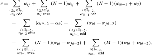
• For (5.25) or (5.26),

  

6.3.26 Example $\texttt {D}_{4,2}$

Here $\texttt {a}_{3, 2} = \{ \{2\}, \{1,3\}, \mathbb {I}_3\}$. We exemplify the incarnation when $j = \theta - j$ in the case $\theta = 4$, $j = 2$. Here is the basic datum:

To describe the incarnation, we need the matrices $(\mathfrak {q}^{(i)})_{i\in \mathbb {I}_6}$, from left to right and from up to down:

Now, this is the incarnation:

6.4 Type ${\mathbf {D}}(2,1;\alpha )$

Here, $q,r,s\ne 1$, $qrs=1$. ${\mathbf {D}}(2,1;\alpha )$, $\alpha \ne 0,-1$, is a Lie superalgebra of superdimension 9|8 [57, Proposition 2.5.6]. There exist 4 pairs $(A, \mathbf {p})$ of (families of) matrices and parity vectors as in Sect. 2.8 such that the corresponding contragredient Lie superalgebra is isomorphic to ${\mathbf {D}}(2,1;\alpha )$.

6.4.1 Basic datum and root system

The basic datum $(\mathcal {X}, \rho )$, where $\mathcal {X}= \{a_j{:}\,j \in \mathbb {I}_4\}$; and the bundle $(C^{a_j})_{j\in \mathbb {I}_4}$ of Cartan matrices are described by the following diagram:

Here the numeration of $A_3$ is as in (4.2) while $A_2^{(1)}$ is as in (3.11) and below. Using the notation (3.1), the bundle of root sets is the following:

$$\begin{aligned} \varDelta _{+}^{a_1}&= \{ 1,12,123,12^23,2,23,3 \}, \quad \varDelta _{+}^{a_2} = s_{12}\big (\varDelta _{+}^{a_1}\big ), \\ \varDelta _{+}^{a_3}&= \{1,12,13,123,2,23,3 \}, \quad \varDelta _{+}^{a_4} = s_{23}\big (\varDelta _{+}^{a_1}\big ). \end{aligned}$$

We denote this generalized root system by $\texttt {D}(2,1)$.

6.4.2 Weyl groupoid

The isotropy group at $a_1 \in \mathcal {X}$ is

$$\begin{aligned} \mathcal {W}(a_1)= \left\langle \varsigma _1^{a_1}, \varsigma _2^{a_1}\varsigma _3 \varsigma _1\varsigma _3 \varsigma _2, \varsigma _3^{a_1} \right\rangle \simeq \mathbb {Z}/2 \times \mathbb {Z}/2 \times \mathbb {Z}/2 \le GL (\mathbb {Z}^\mathbb {I}). \end{aligned}$$

6.4.3 Lie superalgebras realizing this generalized root system

To describe the incarnation in the setting of Lie superalgebras, we need parity vectors $\mathbf {p}=(1,-1,1)$, $\mathbf {p}'=(-1,-1,-1) \in \mathbb {G}_2^3$, and matrices

$$\begin{aligned} {\mathbf {D}}\left( \alpha \right)&:= \begin{pmatrix} 2 &{} -1 &{} 0 \\ 1 &{} 0 &{} \alpha \\ 0 &{} -1 &{} 2 \end{pmatrix},&{\mathbf {D}'}\left( \alpha \right)&:= \begin{pmatrix} 0 &{} 1 &{} -1-\alpha \\ 1 &{} 0 &{} \alpha \\ 1+\alpha &{} -\alpha &{} 0 \end{pmatrix},&\alpha \ne \{0,-1\}. \end{aligned}$$

Let $\alpha \ne \{0,-1\}$. The assignment

$$\begin{aligned} \begin{aligned} a_1&\longmapsto \big ({\mathbf {D}}\left( \alpha \right) , \mathbf {p}\big ),&a_2&\longmapsto s_{12 }\big ({\mathbf {D}}\left( -1-\alpha \right) , \mathbf {p}\big ),\\ a_3&\longmapsto \big ({\mathbf {D}'}\left( \alpha \right) , \mathbf {p}' \big ),&a_4&\longmapsto s_{23}\left( {\mathbf {D}}\left( -1-\alpha ^{-1}\right) , \mathbf {p}\right) , \end{aligned} \end{aligned}$$

(5.42)

provides an isomorphism of generalized root systems, cf. Sect. 2.8. Moreover, the Lie superalgebras associated to $\big ({\mathbf {D}}\left( \alpha \right) , \mathbf {p}\big )$, $\big ({\mathbf {D}}\left( \beta \right) , \mathbf {p}\big )$ if and only if

$$\begin{aligned} \beta \in \left\{ \alpha ^{\pm 1}, -(1+\alpha )^{\pm 1}, -(1+\alpha ^{-1})^{\pm 1}\right\} . \end{aligned}$$

6.4.4 Incarnation

Here is an incarnation of $\texttt {D}(2,1)$:

(5.43)

We set $N=\mathrm{ord}\,q$ (as always), $M=\mathrm{ord}\,r$, $L=\mathrm{ord}\,s$. Also,

$$\begin{aligned} x_{123,2} := [x_{123},x_2]_c. \end{aligned}$$

6.4.5 The generalized Dynkin diagram (5.43 a), $q,r,s\ne -1$

The set

$$\begin{aligned}&\left\{ x_{3}^{n_1} x_{23}^{n_2} x_{2}^{n_{3}} x_{123,2}^{n_4} x_{123}^{n_5} x_{12}^{n_6} x_1^{n_7} \, | \, 0\le n_{1}<M, \, 0\le n_{4}<L, \, 0\le n_7<N,\right. \\&\quad \left. 0\le n_2, n_{3}, n_{5}, n_6 <2\right\} . \end{aligned}$$

is a PBW-basis of ${\mathcal {B}}_{\mathfrak {q}}$. If $N, M, L<\infty$, then

$$\begin{aligned} \dim {\mathcal {B}}_{\mathfrak {q}}= 2^4 LMN . \end{aligned}$$

If exactly two, respectively all, of N, L, M are $\infty$, then

$$\begin{aligned} \mathrm{GK-dim}\,{\mathcal {B}}_{\mathfrak {q}}= 2, \text { respectively } 3. \end{aligned}$$

The set of positive Cartan roots is ${\mathcal {O}}_+^{\mathfrak {q}} = \{1,12^23,3\}$. The Nichols algebra ${\mathcal {B}}_{\mathfrak {q}}$ is generated by $(x_i)_{i\in \mathbb {I}_3}$ with defining relations

$$\begin{aligned} \begin{aligned} x_1^N&=0;&x_2^2&=0;&x_3^M&=0;&x_{123,2}^L&=0;\\ x_{112}&=0;&x_{332}&=0;&x_{13}&=0. \end{aligned} \end{aligned}$$

(5.44)

If $N = \infty$, i.e. $q\notin \mathbb {G}_{\infty }$, respectively $L = \infty$, $M= \infty$, then we omit the relation where it appears as exponent.

The degree of the integral is .

6.4.6 The generalized Dynkin diagram (5.43 a), $q=-1,r,s\ne -1$

The Nichols algebra ${\mathcal {B}}_{\mathfrak {q}}$ is generated by $(x_i)_{i\in \mathbb {I}_3}$ with defining relations

$$\begin{aligned} \begin{aligned} x_1^2&=0;&x_2^2&=0;&x_3^M&=0;&x_{123,2}^L&=0;\\ x_{12}^2&=0;&x_{332}&=0;&x_{13}&=0. \end{aligned} \end{aligned}$$

(5.45)

If $L = \infty$, respectively $M= \infty$, then we omit the relation where it appears as exponent. The PBW basis, the dimension, the GK-dimension, the set of Cartan roots and are as in Sect. 5.4.5.

6.4.7 The generalized Dynkin diagrams (5.43 b and d)

These diagrams are of the shape of (5.43 a) but with s interchanged with q, respectively with r. Hence the corresponding Nichols algebras are as in Sects. 5.4.5 and 5.4.6.

6.4.8 The generalized Dynkin diagram (5.43 c)

The set

$$\begin{aligned}&\left\{ x_{3}^{n_1} x_{23}^{n_2} x_{2}^{n_3} x_{123}^{n_4} x_{13}^{n_5} x_{12}^{n_6} x_1^{n_7} \, | \, 0\le n_{2}<M, \, 0\le n_{6}<L, \, 0\le n_5<N, \right. \\&\quad \left. 0\le n_1, n_{3}, n_{4}, n_7 <2\right\} . \end{aligned}$$

is a PBW-basis of ${\mathcal {B}}_{\mathfrak {q}}$. The dimension and the GK-dimension are as in Sect. 5.4.5.

The set of positive Cartan roots is ${\mathcal {O}}_+^{\mathfrak {q}} = \{12,13,23\}$. The Nichols algebra ${\mathcal {B}}_{\mathfrak {q}}$ is generated by $(x_i)_{i\in \mathbb {I}_3}$ with defining relations

$$\begin{aligned} x_1^2&=0;&x_2^2&=0;&x_3^2&=0; \nonumber \\ x_{12}^N&=0;&x_{23}^M&=0;&x_{13}^L&=0; \end{aligned}$$

(5.46)

$$\begin{aligned} x_{(13)}-\frac{1-s}{q_{23}(1-r)}[x_{13},x_2]_c-q_{12}(1-s)x_2x_{13}=0. \end{aligned}$$

If $N = \infty$, i.e. $q\notin \mathbb {G}_{\infty }$, respectively $L = \infty$, $M= \infty$, then we omit the relation where it appears as exponent. The degree of the integral is

6.4.9 The associated Lie algebra

This is of type $A_1\times A_1\times A_1$.

6.5 Type ${\mathbf {F}}(4)$

Here $N > 3$. ${\mathbf {F}}(4)$ is a Lie superalgebra of superdimension 24|16 [57, Proposition 2.5.6]. There exist 6 pairs $(A, \mathbf {p})$ of matrices and parity vectors as in Sect. 2.8 such that the corresponding contragredient Lie superalgebra is isomorphic to ${\mathbf {F}}(4)$.

6.5.1 Basic datum and root system

Below, $A_4$, $C_4$, $F_4$ and ${}_2T$ are numbered as in (4.2), (4.15), (4.35) and (3.11), respectively. Also, we denote

$$\begin{aligned} \kappa _0 = (1 4)(2 3),\quad \kappa _1 =(1234),\quad \kappa _2 = (234) \in \mathbb {S}_4. \end{aligned}$$

The basic datum and the bundle of Cartan matrices are described the following diagram, that we call $\texttt {F}(4)$:

Using the notation (3.1), the bundle of root sets is the following:

$$\begin{aligned} \varDelta _{+}^{a_1}&= \left\{ 1, 12, 2, 123, 12^23^2, 123^2, 23, 23^2, 3, 12^23^34, 12^23^24, 123^24, 23^24, 12^23^34^2,\right. \\&\quad \left. 1234, 234, 34, 4 \right\} , \\ \varDelta _{+}^{a_2}&= \left\{ 1, 12, 2, 123, 23, 3, 12^23^34, 12^23^24, 123^24, 23^24, 12^23^34^2, 1234, 12^23^24^2,\right. \\&\quad \left. 123^24^2, 234, 23^24^2, 34, 4 \right\} ,\\ \varDelta _{+}^{a_3}&= \left\{ 1, 12, 2, 123, 23, 3, 12^234, 12^24, 1234, 12^23^24^2, 234, 12^234^2, 34, 1234^2,\right. \\&\quad \left. 124, 234^2, 24, 4 \right\} , \\ \varDelta _{+}^{a_4}&= s_{13} \left( \left\{ 1, 12, 2, 12^23, 123, 12^23^2, 23, 3, 1^22^33^24, 12^33^24, 12^23^24, 12^234, 1234,\right. \right. \\&\quad \left. \left. 124, 234, 24, 34, 4 \right\} \right) , \\ \varDelta _{+}^{a_5}&= \kappa _1\left( \left\{ 1, 12, 2, 123, 23, 3, 12^23^34, 12^23^24, 1^22^33^44^2, 123^24, 12^33^44^2, 12^23^44^2, \right. \right. \\&\quad \left. \left. 23^24, 12^23^34^2,1234, 234, 34, 4 \right\} \right) ,\\ \varDelta _{+}^{a_6}&= \kappa _2 \left( \left\{ 1, 12, 12^2, 2, 12^23, 123, 23, 3, 1^22^33^24, 12^33^24, 12^23^24, 123^24, 12^234, \right. \right. \\&\quad \left. \left. 1234, 23^24, 234, 34, 4 \right\} \right) . \end{aligned}$$

6.5.2 Weyl groupoid

The isotropy group at $a_1 \in \mathcal {X}$ is

$$\begin{aligned} \mathcal {W}(a_1)= \left\langle \varsigma _1^{a_1}, \varsigma _2^{a_1}, \varsigma _3^{a_1}, \varsigma _4^{a_1}\varsigma _3 \varsigma _2 \varsigma _1 \varsigma _4 \varsigma _1 \varsigma _2 \varsigma _3 \varsigma _4 \right\rangle \simeq W(B_3) \times \mathbb {Z}/2 \le GL (\mathbb {Z}^\mathbb {I}). \end{aligned}$$

6.5.3 Lie superalgebras realizing this generalized root system

To describe the incarnation in the setting of Lie superalgebras, we need parity vectors $\mathbf {p}_{{\mathbb {J}}}$ as in (5.6), ${\mathbb {J}}\subset \mathbb {I}$, and matrices

$$\begin{aligned} A_1&=\left( {\begin{matrix} 2 &{} -1 &{} 0 &{} 0 \\ -1 &{} 2 &{} -1 &{} 0 \\ 0 &{} -2 &{} 2 &{} -1 \\ 0 &{} 0 &{} 1 &{} 0 \end{matrix}} \right) ,&A_2&=\left( {\begin{matrix} 2 &{} -1 &{} 0 &{} 0 \\ -1 &{} 2 &{} -1 &{} 0 \\ 0 &{} -2 &{} 0 &{} 1 \\ 0 &{} 0 &{} 1 &{} 0 \end{matrix}} \right) ,&A_3&=\left( {\begin{matrix} 2 &{} -1 &{} 0 &{} 0 \\ -1 &{} 0 &{} 2 &{} 1 \\ 0 &{} -2 &{} 0 &{} 1 \\ 0 &{} -1 &{} -1 &{} 2 \end{matrix}} \right) ,\\ A_4&=\left( {\begin{matrix} 0 &{} 2 &{} 0 &{} -3 \\ 2 &{} 0 &{} -2 &{} 1 \\ 0 &{} -1 &{} 2 &{} 0 \\ 3 &{} 1 &{} 0 &{} 0 \end{matrix}} \right) ,&A_5&=\left( {\begin{matrix} 2 &{} 0 &{} 0 &{} -1 \\ 0 &{} 2 &{} -2 &{} -1 \\ 0 &{} -1 &{} 2 &{} 0 \\ 3 &{} -1 &{} 0 &{} 0 \end{matrix}} \right) ,&A_6&=\left( {\begin{matrix} 0 &{} 2 &{} 0 &{} 3 \\ -1 &{} 2 &{} -1 &{} 0 \\ 0 &{} -1 &{} 2 &{} 0 \\ -1 &{} 0 &{} 0 &{} 2 \end{matrix}} \right) . \end{aligned}$$

The assignment

$$\begin{aligned} \begin{aligned} a_1&\longmapsto \big (A_1, \mathbf {p}_{\{4\}}\big ),&a_2&\longmapsto \big (A_2, \mathbf {p}_{\{3,4\}}\big ),&a_3&\longmapsto \big (A_3, \mathbf {p}_{\{2,3\}}\big ),\\ a_4&\longmapsto \big (A_4, \mathbf {p}_{\{1,2,4\}}\big ),&a_5&\longmapsto \big (A_5, \mathbf {p}_{\{1\}}\big ),&a_6&\longmapsto \big (A_6, \mathbf {p}_{\{4\}}\big ), \end{aligned} \end{aligned}$$

(5.47)

provides an isomorphism of generalized root systems, cf. Sect. 2.8.

6.5.4 Incarnation

Here it is:

(5.48)

6.5.5 PBW-basis and (GK-)dimension

Notice that the roots in each $\varDelta _{+}^{a_i}$, $i\in \mathbb {I}_6$, are ordered from left to right, justifying the notation $\beta _1, \ldots , \beta _{18}$.

The root vectors $x_{\beta _k}$ are described as in Remark 2.14. Thus

$$\begin{aligned} \left\{ x_{\beta _{18}}^{n_{18}} x_{\beta _{17}}^{n_{17}} \ldots x_{\beta _2}^{n_{2}} x_{\beta _1}^{n_{1}} \, | \, 0\le n_{k}<N_{\beta _k} \right\} . \end{aligned}$$

is a PBW-basis of ${\mathcal {B}}_{\mathfrak {q}}$. Let $L=\mathrm{ord}\,q^3$, $M=\mathrm{ord}\,q^2$. If $N<\infty$, then

$$\begin{aligned} \dim {\mathcal {B}}_{\mathfrak {q}}= 2^8LM^3N^6. \end{aligned}$$

If $N=\infty$ (that is, if q is not a root of unity), then $\mathrm{GK-dim}\,{\mathcal {B}}_{\mathfrak {q}}= 10$.

6.5.6 The generalized Dynkin diagram (5.48 a), $N> 4$

The Nichols algebra ${\mathcal {B}}_{\mathfrak {q}}$ is generated by $(x_i)_{i\in \mathbb {I}_4}$ with defining relations

$$\begin{aligned} \begin{aligned} x_{13}&=0;&x_{14}&=0;&x_{24}&=0; \\ x_{112}&=0;&x_{221}&=0;&x_{223}&=0; \quad x_{334}=0;\\ x_{3332}&=0;&x_{4}^2&=0;&x_\alpha ^{N_\alpha }&=0, \ \alpha \in {\mathcal {O}}_+^{\mathfrak {q}}; \end{aligned} \end{aligned}$$

(5.49)

where ${\mathcal {O}}_+^{\mathfrak {q}}=\{1,12, 2, 123, 12^23^2, 123^2, 23, 23^2, 3, 12^23^34^2 \}$. If $N = \infty$, i.e. $q\notin \mathbb {G}_{\infty }$, then we omit the last set of relations. Here

6.5.7 The generalized Dynkin diagram (5.48 a), $N =4$

The Nichols algebra ${\mathcal {B}}_{\mathfrak {q}}$ is generated by $(x_i)_{i\in \mathbb {I}_4}$ with defining relations

$$\begin{aligned} \begin{aligned} x_{13}&=0;&x_{14}&=0;&[x_{(13)},x_2]_c=0; \\ x_{334}&=0;&x_{24}&=0;&[x_{23},x_{(24)}]_c=0; \\ x_{3332}&=0;&x_{4}^2&=0;&x_\alpha ^{N_\alpha }=0, \ \alpha \in {\mathcal {O}}_+^{\mathfrak {q}}; \end{aligned} \end{aligned}$$

(5.50)

here, ${\mathcal {O}}_+^{\mathfrak {q}}$, are as in Sect. 5.5.6.

6.5.8 The generalized Dynkin diagram (5.48 b), $N> 4$

The Nichols algebra ${\mathcal {B}}_{\mathfrak {q}}$ is generated by $(x_i)_{i\in \mathbb {I}_4}$ with defining relations

$$\begin{aligned} \begin{aligned} x_{13}&=0;&x_{14}&=0;&x_{24}=0; \quad x_{112}=0;\\ x_{221}&=0;&x_{223}&=0;&\left[ [x_{43},x_{432}]_c,x_3\right] _c=0;\\ x_{3}^2&=0;&x_{4}^2&=0;&x_\alpha ^{N_\alpha }=0, \ \alpha \in {\mathcal {O}}_+^{\mathfrak {q}}; \end{aligned} \end{aligned}$$

(5.51)

where ${\mathcal {O}}_+^{\mathfrak {q}}=\{1, 12, 2, 12^23^34, 1234, 12^23^24^2, 123^24^2, 234, 23^24^2, 34 \}$. If $N = \infty$, i.e. $q\notin \mathbb {G}_{\infty }$, then we omit the last set of relations. Here

6.5.9 The generalized Dynkin diagram (5.48 b), $N =4$

The Nichols algebra ${\mathcal {B}}_{\mathfrak {q}}$ is generated by $(x_i)_{i\in \mathbb {I}_4}$ with defining relations

$$\begin{aligned} \begin{aligned} &x_{13} = 0;\qquad x_{14} = 0;\qquad[x_{(13)},x_2]_c=0; \\ &x_{24} = 0;\qquad x_{23}^2 = 0;\qquad[[x_{43},x_{432}]_c,x_3]_c=0; \\ &x_{3}^2 = 0;\qquad x_{4}^2 = 0;\qquad x_\alpha ^{N_\alpha }=0, \ \alpha \in {\mathcal {O}}_+^{\mathfrak {q}}; \end{aligned} \end{aligned}$$

(5.52)

here, ${\mathcal {O}}_+^{\mathfrak {q}}$, are as in Sect. 5.5.8.

6.5.10 The generalized Dynkin diagram (5.48 c), $N>4$

The Nichols algebra ${\mathcal {B}}_{\mathfrak {q}}$ is generated by $(x_i)_{i\in \mathbb {I}_4}$ with defining relations

$$\begin{aligned}&\begin{aligned} x_{13}&=0;&x_{14}&=0;\quad x_{112}=0; \\ x_{442}&=0;&x_{443}&=0;\quad [x_{(13)},x_2]_c=0; \\ x_{2}^2&=0;&x_{3}^2&=0;\quad x_\alpha ^{N_\alpha }=0, \ \alpha \in {\mathcal {O}}_+^{\mathfrak {q}}; \end{aligned} \\&x_{(24)}- q_{34}q[x_{24},x_3]_c-q_{23}(1-q^{-1})x_3x_{24}=0; \end{aligned}$$

(5.53)

where ${\mathcal {O}}_+^{\mathfrak {q}}=\{1, 123, 23, 12^24, 1234, 12^23^24^2, 234, 1234^2, 234^2, 4 \}$. If $N = \infty$, i.e. $q\notin \mathbb {G}_{\infty }$, then we omit the relations $x_\alpha ^{N_\alpha }=0,$ $\alpha \in {\mathcal {O}}_+^{\mathfrak {q}}$. Here

6.5.11 The generalized Dynkin diagram (5.48 c), $N =4$

The Nichols algebra ${\mathcal {B}}_{\mathfrak {q}}$ is generated by $(x_i)_{i\in \mathbb {I}_4}$ with defining relations

$$\begin{aligned}&\begin{aligned} x_{13}&=0;&x_{14}&=0;\quad x_{12}^2=0; \\ x_{442}&=0;&x_{443}&=0;\quad [x_{(13)},x_2]_c=0; \\ x_{2}^2&=0;&x_{3}^2&=0;\quad x_\alpha ^{N_\alpha }=0, \ \alpha \in {\mathcal {O}}_+^{\mathfrak {q}}; \end{aligned} \\&x_{(24)}- q_{34}q[x_{24},x_3]_c-q_{23}(1-q^{-1})x_3x_{24}=0; \end{aligned}$$

(5.54)

here, ${\mathcal {O}}_+^{\mathfrak {q}}$, are as in Sect. 5.5.10.

6.5.12 The generalized Dynkin diagram (5.48 d), $N> 4$

The Nichols algebra ${\mathcal {B}}_{\mathfrak {q}}$ is generated by $(x_i)_{i\in \mathbb {I}_4}$ with defining relations

$$\begin{aligned}&\begin{aligned} x_{13}&=0;&x_{14}&=0;\quad [x_{124},x_2]_c=0; \\ x_{112}&=0;&x_{4}^2&=0;\quad [[x_{32},x_{321}]_c,x_2]_c=0; \\ x_{2}^2&=0;&x_{3}^2&=0;\quad x_\alpha ^{N_\alpha }=0, \ \alpha \in {\mathcal {O}}_+^{\mathfrak {q}}; \end{aligned} \\&x_{(24)}+ q_{34}\frac{1-q^3}{1-q^2}[x_{24},x_3]_c-q_{23}(1-q^{-3})x_3x_{24}=0; \end{aligned}$$

(5.55)

where ${\mathcal {O}}_+^{\mathfrak {q}}=\{1,123, 12^23^2, 23, 1^22^33^24, 12^33^24, 12^234, 124, 24, 34\}$. If $N = \infty$, i.e. $q\notin \mathbb {G}_{\infty }$, then we omit the relations $x_\alpha ^{N_\alpha }=0,$ $\alpha \in {\mathcal {O}}_+^{\mathfrak {q}}$. Here

6.5.13 The generalized Dynkin diagram (5.48 d), $N =4$

The Nichols algebra ${\mathcal {B}}_{\mathfrak {q}}$ is generated by $(x_i)_{i\in \mathbb {I}_4}$ with defining relations

$$\begin{aligned}&\begin{aligned} x_{13}&=0;&x_{14}&=0;\quad [x_{124},x_2]_c=0; \\ x_{12}^2&=0;&x_{4}^2&=0;\quad [[x_{32},x_{321}]_c,x_2]_c=0; \\ x_{2}^2&=0;&x_{3}^2&=0;\quad x_\alpha ^{N_\alpha }=0, \ \alpha \in {\mathcal {O}}_+^{\mathfrak {q}}; \end{aligned} \\&x_{(24)}+ q_{34}\frac{1-q^3}{1-q^2}[x_{24},x_3]_c-q_{23}(1-q^{-3})x_3x_{24}=0; \end{aligned}$$

(5.56)

here, ${\mathcal {O}}_+^{\mathfrak {q}}$, are as in Sect. 5.5.12.

6.5.14 The generalized Dynkin diagram (5.48 e), $N\ne 4,6$

The Nichols algebra ${\mathcal {B}}_{\mathfrak {q}}$ is generated by $(x_i)_{i\in \mathbb {I}_4}$ with defining relations

$$\begin{aligned} \begin{aligned} x_{13}&=0;&x_{14}&=0;\quad x_{24}=0; \quad x_{112}=0; \\ x_{221}&=0;&x_{223}&=0;\quad \left[ \left[ [x_{432},x_3]_c,[x_{4321},x_3]_c\right] _c,x_{32}\right] _c=0;\\ x_{443}&=0;&x_{3}^2&=0;\quad x_\alpha ^{N_\alpha }=0, \ \alpha \in {\mathcal {O}}_+^{\mathfrak {q}}; \end{aligned} \end{aligned}$$

(5.57)

where ${\mathcal {O}}_+^{\mathfrak {q}}=\{1,12, 2, 12^23^24, 1^22^33^44^2, 123^24, 12^33^44^2, 12^23^44^2, 23^24, 4 \}$. If $N = \infty$, i.e. $q\notin \mathbb {G}_{\infty }$, then we omit the last set of relations. Here

6.5.15 The generalized Dynkin diagram (5.48 e), $N =6$

The Nichols algebra ${\mathcal {B}}_{\mathfrak {q}}$ is generated by $(x_i)_{i\in \mathbb {I}_4}$ with defining relations

$$\begin{aligned} \begin{aligned} x_{13}&=0;&x_{14}&=0;\quad x_{24}=0; \quad x_{112}=0; \\ x_{221}&=0;&x_{223}&=0;\quad\left[ [[x_{432},x_3]_c,[x_{4321},x_3]_c]_c,x_{32}\right] _c=0;\\ x_{34}^2&=0;&x_{3}^2&=0;\quad x_\alpha ^{N_\alpha }=0, \ \alpha \in {\mathcal {O}}_+^{\mathfrak {q}}; \end{aligned} \end{aligned}$$

(5.58)

here, ${\mathcal {O}}_+^{\mathfrak {q}}$, are as in Sect. 5.5.17.

6.5.16 The generalized Dynkin diagram (5.48 e), $N =4$

The Nichols algebra ${\mathcal {B}}_{\mathfrak {q}}$ is generated by $(x_i)_{i\in \mathbb {I}_4}$ with defining relations

$$\begin{aligned} \begin{aligned} x_{13}&=0;&x_{14}&=0;\quad [x_{(13)},x_2]_c=0; \\ x_{24}&=0;&x_{443}&=0;\quad \left[ [[x_{432},x_3]_c,[x_{4321},x_3]_c]_c,x_{32}\right] _c=0;\\ x_{23}^2&=0;&x_{3}^2&=0;\quad x_\alpha ^{N_\alpha }=0, \ \alpha \in {\mathcal {O}}_+^{\mathfrak {q}}; \end{aligned} \end{aligned}$$

(5.59)

here, ${\mathcal {O}}_+^{\mathfrak {q}}$, are as in Sect. 5.5.14.

6.5.17 The generalized Dynkin diagram (5.48 f), $N\ne 4,6$

The Nichols algebra ${\mathcal {B}}_{\mathfrak {q}}$ is generated by $(x_i)_{i\in \mathbb {I}_4}$ with defining relations

$$\begin{aligned}&\begin{aligned} x_{13}&=0;&x_{14}&=0;&x_{24}&=0; \\ x_{112}&=0;&x_{2221}&=0;&x_{223}&=0; \\ x_{443}&=0;&x_{3}^2&=0;&x_\alpha ^{N_\alpha }&=0, \ \alpha \in {\mathcal {O}}_+^{\mathfrak {q}}; \end{aligned}\nonumber \\&[[x_{(14)},x_2]_c,x_3]_c-q_{23}(q^2-q)[[x_{(14)},x_3]_c,x_2]_c=0; \end{aligned}$$

(5.60)

where ${\mathcal {O}}_+^{\mathfrak {q}}=\{ 1, 12, 12^2, 2, 1^22^33^24, 12^33^24, 12^23^24, 123^24, 23^24, 4 \}$. If $N = \infty$, i.e. $q\notin \mathbb {G}_{\infty }$, then we omit the relations $x_\alpha ^{N_\alpha }=0,$ $\alpha \in {\mathcal {O}}_+^{\mathfrak {q}}$. Here

6.5.18 The generalized Dynkin diagram (5.48 f), $N =6$

The Nichols algebra ${\mathcal {B}}_{\mathfrak {q}}$ is generated by $(x_i)_{i\in \mathbb {I}_4}$ with defining relations

$$\begin{aligned}&\begin{aligned} x_{13}&=0;&x_{14}&=0;&x_{24}&=0; \\ x_{112}&=0;&x_{2221}&=0;&x_{223}&=0; \\ x_{34}^2&=0;&x_{3}^2&=0;&x_\alpha ^{N_\alpha }&=0, \ \alpha \in {\mathcal {O}}_+^{\mathfrak {q}}; \end{aligned}\nonumber \\&[[x_{(14)},x_2]_c,x_3]_c-q_{23}(q^2-q)[[x_{(14)},x_3]_c,x_2]_c=0; \end{aligned}$$

(5.61)

here, ${\mathcal {O}}_+^{\mathfrak {q}}$, are as in Sect. 5.5.17.

6.5.19 The generalized Dynkin diagram (5.48 f), $N =4$

The Nichols algebra ${\mathcal {B}}_{\mathfrak {q}}$ is generated by $(x_i)_{i\in \mathbb {I}_4}$ with defining relations

$$\begin{aligned}&\begin{aligned} x_{13}&=0;&x_{14}&=0;&x_{24}&=0; \\ x_{223}&=0;&x_{2221}&=0;&[x_{12}&,x_{(13)}]_c=0; \\ x_{443}&=0;&x_{3}^2&=0;&x_\alpha ^{N_\alpha }&=0, \ \alpha \in {\mathcal {O}}_+^{\mathfrak {q}}; \end{aligned}\nonumber \\&\quad [[x_{(14)},x_2]_c,x_3]_c-q_{23}(q^2-q)[[x_{(14)},x_3]_c,x_2]_c=0; \end{aligned}$$

(5.62)

here, ${\mathcal {O}}_+^{\mathfrak {q}}$, are as in Sect. 5.5.17.

6.5.20 The associated Lie algebra

This is of type $A_1\times B_3$.

6.6 Type ${\mathbf {G}}(3)$

Here $N > 3$. ${\mathbf {G}}(3)$ is a Lie superalgebra (over a field of characteristic $\ne 2,3$) of superdimension 17|14 [57, Proposition 2.5.6]. There exist 4 pairs $(A, \mathbf {p})$ of matrices and parity vectors as in Sect. 2.8 such that the corresponding contragredient Lie superalgebra is isomorphic to ${\mathbf {G}}(3)$.

6.6.1 Basic datum and root system

Below, $A_3$, $B_3$, $D_{4}^{(3)}$ and $T^{(2)}$ are numbered as in (4.2), (4.7), (3.8) and (3.12), respectively. Also, we denote $\kappa = (123) \in \mathbb {S}_3$. The basic datum and the bundle of Cartan matrices are described by the following diagram, that we call $\texttt {G}(3)$:

Using the notation (3.1), the bundle of root sets is the following:

$$\begin{aligned} \varDelta _+^{a_1}&= \left\{ 1,12,123,12^23,12^33,12^33^2,12^43^2,2,23,2^23,3,2^33,2^33^2 \right\} , \\ \varDelta _+^{a_2}&= \left\{ 1,12,23,12^23,1^22^33,1^22^33^2,1^32^43^2,2,123,1^22^23,3,1^32^33,1^32^33^2\right\} , \\ \varDelta _+^{a_3}&= \left\{ 12,1,3,13,1^23,1^223^2,1^323^2,2,123,1^223,23,1^323,1^32^23^2 \right\} , \\ \varDelta _+^{a_4}&= \left\{ 123^2,13,3,1,1^23,1^223,1^323^2,23,123,1^223^2,2,1^323^3,1^32^23^3\right\} . \end{aligned}$$

6.6.2 Weyl groupoid

The isotropy group at $a_1 \in \mathcal {X}$ is

$$\begin{aligned} \mathcal {W}(a_1)= \left\langle \varsigma _1^{a_1}\varsigma _2 \varsigma _3\varsigma _1 \varsigma _3 \varsigma _2 \varsigma _1, \varsigma _2^{a_1}, \varsigma _3^{a_1} \right\rangle \simeq \mathbb {Z}/2 \times W(G_2). \end{aligned}$$

6.6.3 Lie superalgebras realizing this generalized root system

To describe the incarnation in the setting of Lie superalgebras, we need parity vectors $\mathbf {p}_{{\mathbb {J}}}$ as in (5.6), ${\mathbb {J}}\subset \mathbb {I}$, and matrices

$$\begin{aligned} A_1&=\left( {\begin{matrix} 0 &{} 1 &{} 0 \\ -1 &{} 2 &{} -3 \\ 0 &{} -1 &{} 2 \end{matrix}} \right) ,&A_2&=\left( {\begin{matrix} 0 &{} 1 &{} 0 \\ 1 &{} 0 &{} -3 \\ 0 &{} -1 &{} 2 \end{matrix}} \right) ,&A_3&=\left( {\begin{matrix} 2 &{} -1 &{} -2 \\ 1 &{} 0 &{} -3 \\ 1 &{} 1 &{} 0 \end{matrix}} \right) ,&A_4&=\left( {\begin{matrix} 2 &{} 0 &{} -2 \\ 0 &{} 2 &{} -1 \\ 1 &{} 3 &{} 0 \end{matrix}} \right) . \end{aligned}$$

The assignment

$$\begin{aligned} \begin{aligned} a_1&\mapsto \big (A_1, \mathbf {p}_{\{1\}}\big ),&a_2&\mapsto \big (A_2, \mathbf {p}_{\{1,2\}}\big ),\\ a_3&\mapsto \big (A_3, \mathbf {p}_{\{2,3\}}\big ),&a_4&\mapsto \big (A_4, \mathbf {p}_{\{1,3\}}\big ), \end{aligned} \end{aligned}$$

(5.63)

provides an isomorphism of generalized root systems, cf. Sect. 2.8.

6.6.4 Incarnation

Here it is:

(5.64)

6.6.5 PBW-basis and (GK-)dimension

Notice that the roots in each $\varDelta _{+}^{a_i}$, $i\in \mathbb {I}_4$, are ordered from left to right, justifying the notation $\beta _1, \ldots , \beta _{13}$.

The root vectors $x_{\beta _k}$ are described as in Remark 2.14. Thus

$$\begin{aligned} \left\{ x_{\beta _{13}}^{n_{13}} x_{\beta _{12}}^{n_{12}} \ldots x_{\beta _2}^{n_{2}} x_{\beta _1}^{n_{1}} \, | \, 0\le n_{k}<N_{\beta _k} \right\} . \end{aligned}$$

is a PBW-basis of ${\mathcal {B}}_{\mathfrak {q}}$. Let $L=\mathrm{ord}\,-q$, $M=\mathrm{ord}\,q^3$. If $N<\infty$, then

$$\begin{aligned} \dim {\mathcal {B}}_{\mathfrak {q}}= 2^6LM^3N^3. \end{aligned}$$

If $N=\infty$ (that is, if q is not a root of unity), then $\mathrm{GK-dim}\,{\mathcal {B}}_{\mathfrak {q}}= 7$.

6.6.6 The generalized Dynkin diagram (5.64 a), $N\ne 4,6$

The Nichols algebra ${\mathcal {B}}_{\mathfrak {q}}$ is generated by $(x_i)_{i\in \mathbb {I}_3}$ with defining relations

$$\begin{aligned} \begin{aligned} x_{13}&=0;&x_{221}&=0;&x_{332}&=0; \\ x_{22223}&=0;&x_{1}^2&=0;&x_{\alpha }^{N_\alpha }&=0, \ \alpha \in {\mathcal {O}}_+^{\mathfrak {q}}; \end{aligned} \end{aligned}$$

(5.65)

where ${\mathcal {O}}_+^{\mathfrak {q}}=\{2,3,23,2^23,2^33,12^23,2^33^2\}$. If $N = \infty$, i.e. $q\notin \mathbb {G}_{\infty }$, then we omit the last set of relations. Here

6.6.7 The generalized Dynkin diagram (5.64 a), $N =6$

The Nichols algebra ${\mathcal {B}}_{\mathfrak {q}}$ is generated by $(x_i)_{i\in \mathbb {I}_3}$ with defining relations

$$\begin{aligned} \begin{aligned} x_{13}&=0;&x_{221}&=0;&[x_{12},x_{(13)}]_c=0; \\ x_{22223}&=0;&x_{1}^2&=0;&x_{\alpha }^{N_\alpha }=0, \ \alpha \in {\mathcal {O}}_+^{\mathfrak {q}}; \end{aligned} \end{aligned}$$

(5.66)

here, ${\mathcal {O}}_+^{\mathfrak {q}}$, are as in Sect. 5.6.6.

6.6.8 The generalized Dynkin diagram (5.64 a), $N =4$

The Nichols algebra ${\mathcal {B}}_{\mathfrak {q}}$ is generated by $(x_i)_{i\in \mathbb {I}_3}$ with defining relations

$$\begin{aligned} \begin{aligned} x_{13}&=0;&x_{221}&=0;&[[[x_{(13)},&x_2]_c,x_2]_c,x_2]_c=0; \\ x_{332}&=0;&x_{1}^2&=0;&x_{\alpha }^{N_\alpha }&=0, \ \alpha \in {\mathcal {O}}_+^{\mathfrak {q}}; \end{aligned} \end{aligned}$$

(5.67)

here, ${\mathcal {O}}_+^{\mathfrak {q}}$, are as in Sect. 5.6.6.

6.6.9 The generalized Dynkin diagram (5.64 b), $N\ne 6$

The Nichols algebra ${\mathcal {B}}_{\mathfrak {q}}$ is generated by $(x_i)_{i\in \mathbb {I}_3}$ with defining relations

$$\begin{aligned} \begin{aligned} x_{13}&=0;&x_{332}&=0;&[[x_{12},&[x_{12},x_{(13)}]_c]_c,x_2]_c=0; \\ x_{1}^2&=0;&x_{2}^2&=0;&x_{\alpha }^{N_\alpha }&=0, \ \alpha \in {\mathcal {O}}_+^{\mathfrak {q}}; \end{aligned} \end{aligned}$$

(5.68)

where ${\mathcal {O}}_+^{\mathfrak {q}}=\{3,12,123,12^23,1^22^23,1^32^33,1^32^33^2\}$. If $N = \infty$, i.e. $q\notin \mathbb {G}_{\infty }$, then we omit the last set of relations. Here

6.6.10 The generalized Dynkin diagram (5.64 b), $N =6$

The Nichols algebra ${\mathcal {B}}_{\mathfrak {q}}$ is generated by $(x_i)_{i\in \mathbb {I}_3}$ with defining relations

$$\begin{aligned} \begin{aligned} x_{13}&=0;&x_{23}^2&=0;&[[x_{12},&[x_{12},x_{(13)}]_c]_c,x_2]_c=0; \\ x_{1}^2&=0;&x_{2}^2&=0;&x_{\alpha }^{N_\alpha }&=0, \ \alpha \in {\mathcal {O}}_+^{\mathfrak {q}}; \end{aligned} \end{aligned}$$

(5.69)

here, ${\mathcal {O}}_+^{\mathfrak {q}}$, are as in Sect. 5.6.9.

6.6.11 The generalized Dynkin diagram (5.64 c), $N\ne 6$

The Nichols algebra ${\mathcal {B}}_{\mathfrak {q}}$ is generated by $(x_i)_{i\in \mathbb {I}_3}$ with defining relations

$$\begin{aligned} \begin{aligned} x_{13}&=0; \quad x_{332}=0; \quad x_{1112}=0; \quad x_{2}^2=0; \quad x_{\alpha }^{N_\alpha }=0, \ \alpha \in {\mathcal {O}}_+^{\mathfrak {q}};\\ [x_1,&[x_{123},x_2]_c]_c = \frac{q_{12}q_{32}}{1+q}[x_{12},x_{123}]_c-(q^{-1}-q^{-2})q_{12}q_{13} x_{123}x_{12}; \end{aligned} \end{aligned}$$

(5.70)

where ${\mathcal {O}}_+^{\mathfrak {q}}=\{1,3,12,123,1^22^23,1^32^33,1^32^33^2\}$. If $N = \infty$, i.e. $q\notin \mathbb {G}_{\infty }$, then we omit the relations $x_\alpha ^{N_\alpha }=0,$ $\alpha \in {\mathcal {O}}_+^{\mathfrak {q}}$. Here

6.6.12 The generalized Dynkin diagram (5.64 c), $N =6$

The Nichols algebra ${\mathcal {B}}_{\mathfrak {q}}$ is generated by $(x_i)_{i\in \mathbb {I}_3}$ with defining relations

$$\begin{aligned} \begin{aligned} x_{13}&=0; \ \ x_{23}^2=0; \ \ [x_{112},x_{12}]_c=0; \quad x_{2}^2=0; \quad x_{\alpha }^{N_\alpha }=0, \ \alpha \in {\mathcal {O}}_+^{\mathfrak {q}};\\ [x_1,&[x_{123},x_2]_c]_c = \frac{q_{12}q_{32}}{1+q}[x_{12},x_{123}]_c-(q^{-1}-q^{-2})q_{12}q_{13} x_{123}x_{12}; \end{aligned} \end{aligned}$$

(5.71)

here, ${\mathcal {O}}_+^{\mathfrak {q}}$, are as in Sect. 5.6.11.

6.6.13 The generalized Dynkin diagram (5.64 d)

The Nichols algebra ${\mathcal {B}}_{\mathfrak {q}}$ is generated by $(x_i)_{i\in \mathbb {I}_3}$ with defining relations

$$\begin{aligned} \begin{aligned} x_{1112}&=0; \quad x_{2}^2=0; \quad x_3^2=0; \quad x_{\alpha }^{N_\alpha }=0, \ \alpha \in {\mathcal {O}}_+^{\mathfrak {q}};\\ x_{113}&=0; \ \ x_{(13)}+q^{-2}q_{23}\frac{1-q^3}{1-q}[x_{13},x_2]_c-q_{12}(1-q^3)x_2x_{13}=0; \end{aligned} \end{aligned}$$

(5.72)

where ${\mathcal {O}}_+^{\mathfrak {q}}=\{1,12,23,123,1^223,1^323,1^32^23^2\}$. If $N = \infty$, i.e. $q\notin \mathbb {G}_{\infty }$, then we omit the relations $x_\alpha ^{N_\alpha }=0,$ $\alpha \in {\mathcal {O}}_+^{\mathfrak {q}}$. Here

6.6.14 The associated Lie algebra

This is of type $A_1\times G_2$.

7 Standard type

7.1 Standard type $B_{\theta , j}$, $\theta \ge 2$, $j\in \mathbb {I}_{\theta - 1}$

Here $\zeta \in \mathbb {G}'_3$.

7.1.1 Basic datum and root system

The basic datum is $(\texttt {B}_{\theta , j}, \rho )$ and the root system is ${\mathbf {B}}(j|\theta -j)$, $j\in \mathbb {I}_{\theta -1}$ as in Sect. 5.2.2; hence the Weyl groupoid is as in Sect. 5.2.3. But we have new incarnations.

7.1.2 Incarnation

The assignment

(6.1)

gives an incarnation. Notice that albeit $\theta$ is not a Cartan vertex, $\rho _{\theta } = {\text {id}}$.

7.1.3 PBW-basis and dimension

The root vectors are

$$\begin{aligned} x_{\alpha _{ii}}&= x_{\alpha _{i}} = x_{i},&i \in \mathbb {I}, \\ x_{\alpha _{ij}}&= x_{(ij)} = [x_{i}, x_{\alpha _{(i+1) j}}]_c,&i< j \in \mathbb {I}, \\ x_{\alpha _{i\theta } + \alpha _{\theta }}&= [x_{\alpha _{i\theta }}, x_\theta ]_c,&i \in \mathbb {I}_{\theta - 1},\\ x_{\alpha _{i\theta } + \alpha _{j\theta }}&= [x_{\alpha _{i\theta } + \alpha _{(j+1) \theta }}, x_j]_c,&i < j \in \mathbb {I}_{\theta - 1}, \end{aligned}$$

cf. (2.11). Thus

$$\begin{aligned}&\left\{ x_{\theta }^{n_{\theta \theta }} x_{\alpha _{\theta -1\theta } + \alpha _{\theta \theta }}^{m_{\theta -1\theta }} x_{\alpha _{\theta -1\theta }}^{n_{\theta -1 \theta }} x_{ \theta -1}^{n_{\theta -1 \theta -1}} \ldots x_{\alpha _{1\theta } + \alpha _{2\theta }}^{m_{12}} \ldots x_{\alpha _{1\theta } + \alpha _{\theta \theta }}^{m_{1\theta }} \ldots x_{\alpha _{1\theta }}^{n_{1 \theta }} \ldots x_{1}^{n_{1 1}} \, \right. \\&\quad \left. | \, 0\le n_{ij}<N_{\alpha _{ij}}; \, 0\le m_{ij}<N_{\alpha _{i\theta }+\alpha _{j\theta }}\right\} \end{aligned}$$

is a PBW-basis of ${\mathcal {B}}_{\mathfrak {q}}$. Hence

$$\begin{aligned} \dim {\mathcal {B}}_{\mathfrak {q}}= 2^{\theta (\theta -1)} 3^{j^2+(\theta -j)^2}. \end{aligned}$$

7.1.4 Presentation

The set of positive Cartan roots is

$$\begin{aligned} {\mathcal {O}}_+^{\mathfrak {q}} =&\left\{ \alpha _{ij}, \alpha _{i\theta }+ \alpha _{(j+1)\theta }{:}\,i\le j\in \mathbb {I}_{\theta - 1}, \alpha _{ij} \text { even}\right\} . \end{aligned}$$

(6.2)

Assume that $\theta = 2$. Then ${\mathcal {O}}_+^{\mathfrak {q}} = \{\alpha _{1}, \alpha _{1}+ 2\alpha _{2}\}$ if $\alpha _{1}$ is even, i.e. ${\mathbb {J}}= \emptyset$, and ${\mathcal {O}}_+^{\mathfrak {q}} = \emptyset$ if $\alpha _{1}$ is odd, i.e. ${\mathbb {J}}= \{1\}$.

The Nichols algebra ${\mathcal {B}}_{\mathfrak {q}}$ is generated by $(x_i)_{i\in \mathbb {I}}$ with defining relations

$$\begin{aligned} \begin{aligned}&x_{ij}= 0,\qquad i < j - 1;\qquad [x_{(i-1i+1)},x_i]_c=0, \qquad \qquad i\in {\mathbb {J}};\\&x_{ii(i\pm 1)}= 0,\quad i\in \mathbb {I}_{\theta -1}-{\mathbb {J}};\quad [x_{\theta \theta (\theta -1)(\theta -2)}, x_{\theta (\theta -1)}]_c=0;\\&x_i^2=0,\qquad i\in {\mathbb {J}};\qquad \qquad [x_{\theta \theta (\theta -1)}, x_{\theta (\theta -1)}]_c=0,\qquad \quad \theta -1\in {\mathbb {J}};\\&x_\theta ^3=0;\qquad\qquad\qquad \qquad x_{\alpha }^6 =0,\qquad \qquad \qquad \qquad \alpha \in {\mathcal {O}}_+^{\mathfrak {q}}. \end{aligned} \end{aligned}$$

(6.3)

7.1.5 The associated Lie algebra and

This is of type $D_j\times D_{\theta -j}$. In this case, the Weyl group of the associated Lie algebra is isomorphic to a proper subgroup of the isotropy group of the Weyl groupoid. Here

7.2 Standard type $G_{2}$

Here $\zeta \in \mathbb {G}'_8$.

7.2.1 Basic datum

This is described by the diagram

7.2.2 Root system

The bundle of Cartan matrices $(C^{a_j})_{j\in \mathbb {I}_3}$ is constant: $C^{a_j}$ is the Cartan matrix of type $G_2$ as in (4.43) for any $j \in \mathbb {I}_3$.

The bundle of root sets $(\varDelta ^{a_j})_{j \in \mathbb {I}_3}$ is constant:

$$\begin{aligned} \varDelta ^{a_j}&=\left\{ \pm \alpha _1,\pm (3\alpha _1+\alpha _2), \pm (2\alpha _1+\alpha _2), \pm (3\alpha _1+2\alpha _2), \pm (\alpha _1+\alpha _2), \pm \alpha _2 \right\} . \end{aligned}$$

7.2.3 Weyl groupoid

The isotropy group at $a_1 \in \mathcal {X}$ is

$$\begin{aligned} \mathcal {W}(a_1)&= \left\langle \varsigma ^{a_1}_1 \varsigma _{2} \varsigma _{1} \varsigma _{2} \varsigma _{1}, \varsigma _2^{a_1} \right\rangle \simeq \mathbb {Z}/2 \times \mathbb {Z}/2 \le GL (\mathbb {Z}^\mathbb {I}). \end{aligned}$$

7.2.4 Incarnation

We assign the following Dynkin diagrams to $a_i$, $i\in \mathbb {I}_3$:

(6.4)

7.2.5 The generalized Dynkin diagram (6.4 a)

The set

$$\begin{aligned} \left\{ x_{2}^{n_1} x_{12}^{n_2} x_{3\alpha _1+2\alpha _2}^{n_{3}}x_{112}^{n_4} x_{1112}^{n_5} x_1^{n_6} \, | \, n_{1}, n_{4}\in \mathbb {I}_{0,7}, \ n_{2}, n_{6 }\in \mathbb {I}_{0,3}, \ n_{3}, n_{5}\in \mathbb {I}_{0,1}\right\} \end{aligned}$$

is a PBW-basis of ${\mathcal {B}}_{\mathfrak {q}}$. Hence $\dim {\mathcal {B}}_{\mathfrak {q}}= 2^24^28^2=4096$.

The Nichols algebra ${\mathcal {B}}_{\mathfrak {q}}$ is generated by $(x_i)_{i\in \mathbb {I}_2}$ with defining relations

$$\begin{aligned} \begin{aligned} x_1^4&=0;&x_{221}&=0;&[x_{3\alpha _1+2\alpha _2}, x_{12}]_c&=0;&x_2^8&=0;&x_{112}^8&=0. \end{aligned} \end{aligned}$$

(6.5)

In this case, ${\mathcal {O}}_+^{\mathfrak {q}}=\{\alpha _2, 2\alpha _1+\alpha _2\}$ and .

7.2.6 The generalized Dynkin diagram (6.4 b)

The set

$$\begin{aligned} \left\{ x_{2}^{n_1} x_{12}^{n_2} x_{3\alpha _1+2\alpha _2}^{n_{3}}x_{112}^{n_4} x_{1112}^{n_5} x_1^{n_6} \, | \, n_{2}, n_{5}\in \mathbb {I}_{0,7}, \, n_{4}, n_{6}\in \mathbb {I}_{0,3}, \, n_{1}, n_{3}\in \mathbb {I}_{0,1}\right\} \end{aligned}$$

is a PBW-basis of ${\mathcal {B}}_{\mathfrak {q}}$. Hence $\dim {\mathcal {B}}_{\mathfrak {q}}= 2^24^28^2=4096$.

The Nichols algebra ${\mathcal {B}}_{\mathfrak {q}}$ is generated by $(x_i)_{i\in \mathbb {I}_2}$ with defining relations

$$\begin{aligned} \begin{aligned} x_1^4&=0;&x_2^2&=0;&[x_1,x_{3\alpha _1+2\alpha _2}]_c+\frac{q_{12}}{1-\zeta }x_{112}^2&=0; \\ x_{12}^8&=0;&x_{1112}^8&=0. \end{aligned} \end{aligned}$$

(6.6)

In this case, ${\mathcal {O}}_+^{\mathfrak {q}}=\{\alpha _1+\alpha _2, 3\alpha _1+\alpha _2\}$. and .

7.2.7 The generalized Dynkin diagram (6.4 c)

The set

$$\begin{aligned} \left\{ x_{2}^{n_1} x_{12}^{n_2} x_{3\alpha _1+2\alpha _2}^{n_{3}}x_{112}^{n_4} x_{1112}^{n_5} x_1^{n_6} \, | \, n_{3}, n_{6}\in \mathbb {I}_{0,7}, \, n_{2}, n_{4}\in \mathbb {I}_{0,3}, \, n_{1}, n_{5}\in \mathbb {I}_{0,1}\right\} \end{aligned}$$

is a PBW-basis of ${\mathcal {B}}_{\mathfrak {q}}$. Hence $\dim {\mathcal {B}}_{\mathfrak {q}}= 2^24^28^2=4096$.

The Nichols algebra ${\mathcal {B}}_{\mathfrak {q}}$ is generated by $(x_i)_{i\in \mathbb {I}_2}$ with defining relations

$$\begin{aligned} \begin{aligned} x_1^8&=0;&x_{11112}&=0;&[x_{3\alpha _1+2\alpha _2}, x_{12}]_c&=0; \\ x_2^2&=0;&x_{3\alpha _1+2\alpha _2}^8&=0. \end{aligned} \end{aligned}$$

(6.7)

In this case, ${\mathcal {O}}_+^{\mathfrak {q}}=\{\alpha _1, 3\alpha _1+2\alpha _2\}$. and .

7.2.8 The associated Lie algebra

This is of type $A_1\times A_1$.

Part III. Arithmetic root systems: modular, UFO

8 Modular type, characteristic 2 or 3

8.1 Type $\texttt {wk}(4)$

Here $\theta = 4$, $q\ne \pm 1$. Let $\mathbb {F}$ be a field of characteristic 2, $\alpha \in \mathbb {F}- \mathbb {F}_2$ and

$$\begin{aligned} A = \begin{pmatrix} 0 &{}\quad 1 &{}\quad 0 &{}\quad 0 \\ 1 &{}\quad 0 &{}\quad 1 &{}\quad 0 \\ 0 &{}\quad \alpha &{}\quad 0 &{}\quad 1 \\ 0 &{}\quad 0 &{}\quad 1 &{}\quad 0 \end{pmatrix} \in \mathbb {F}^{4 \times 4}. \end{aligned}$$

Let $\mathfrak {wk}(4,\alpha ) = \mathfrak {g}(A)$ be the corresponding contragredient Lie algebra. Then $\dim \mathfrak {wk}(4,\alpha ) = 34$ [59]. Notice that there are 4 other matrices $A'$ for which $\mathfrak {wk}(4,\alpha ) \simeq \mathfrak {g}(A')$. Here is the root system $\texttt {wk}(4)$ of $\mathfrak {wk}(4,\alpha )$, see [3] for details.

8.1.1 Basic datum and root system

Below, $A_4$ and ${}_1T$ are numbered as in (4.2) and (3.11), respectively. The basic datum and the bundle of Cartan matrices are described by the following diagram:

Using the notation (3.1), the bundle of root sets is the following:

$$\begin{aligned}&\begin{aligned} \varDelta _{+}^{a_1}&= \big \{ 1, 12, 2, 123, 23, 3, 12^23^34, 12^23^24, 123^24, 23^24, 12^23^34^2, 1234, 234, 34, 4 \big \}, \\ \varDelta _{+}^{a_2}&= \big \{ 1, 12, 2, 123, 23, 3, 12^234, 12^24, 1234, 234, 12^234^2, 34, 124, 24, 4\big \}, \\ \varDelta _{+}^{a_5}&= \big \{ 1, 12, 2, 12^23, 123, 23, 3, 12^23^24, 123^24, 23^24, 12^234, 1234, 234, 34, 4 \big \}, \end{aligned}\\&\begin{aligned} \varDelta _{+}^{a_3}&= s_{13}\big (\varDelta _{+}^{a_2}\big ),&\varDelta _{+}^{a_4}&= \kappa _1\big (\varDelta _{+}^{a_1}\big ),&\varDelta _{+}^{a_6}&= \kappa _2\big (\varDelta _{+}^{a_5}\big ),&\varDelta _{+}^{a_7}&= \kappa _3\big (\varDelta _{+}^{a_1}\big ),\\ \varDelta _{+}^{a_8}&= \kappa _4\big (\varDelta _{+}^{a_2}\big ),&\varDelta _{+}^{a_9}&= s_{24}\big (\varDelta _{+}^{a_2}\big ),&\varDelta _{+}^{a_{10}}&= s_{24}\big (\varDelta _{+}^{a_1}\big ). \end{aligned} \end{aligned}$$

8.1.2 Weyl groupoid

The isotropy group at $a_1 \in \mathcal {X}$ is

$$\begin{aligned} \mathcal {W}(a_1)= \langle \varsigma _1^{a_1},\varsigma _2^{a_1}, \varsigma _3^{a_1}\varsigma _2 \varsigma _1 \varsigma _4 \varsigma _1\varsigma _2\varsigma _3, \varsigma _4^{a_1} \rangle \simeq W(A_2) \times W(A_2). \end{aligned}$$

8.1.3 Incarnation

To describe it, we need the matrices $(\mathfrak {q}^{(i)})_{i\in \mathbb {I}_5}$ corresponding to the following Dynkin diagrams, from left to right and from up to down (also denoted below as a,..., e as customary).

(7.1)

Now, this is the incarnation:

$$\begin{aligned}&a_1 \mapsto \mathfrak {q}^{(1)},\qquad a_2 \mapsto \mathfrak {q}^{(4)},\qquad a_3 \mapsto s_{13}(\mathfrak {q}^{(4)}),\qquad a_4 \mapsto \kappa _1(\mathfrak {q}^{(1)}), \\& \qquad \qquad \quad a_5\mapsto s_{34}(\mathfrak {q}^{(3)}),\quad a_6 \mapsto \kappa _2(\mathfrak {q}^{(3)}),&\\& a_7 \mapsto \kappa _3(\mathfrak {q}^{(2)}),\quad a_8 \mapsto \kappa _4(\mathfrak {q}^{(5)}),\quad a_9 \mapsto s_{24}(\mathfrak {q}^{(5)}),\quad a_{10} \mapsto s_{24}(\mathfrak {q}^{(2)}).&\end{aligned}$$

We set $N=\mathrm{ord}\,q$, $M=\mathrm{ord}\,-q^{-1}$.

8.1.4 PBW-basis and (GK-)dimension

Notice that the roots in each $\varDelta _{+}^{a_i}$, $i\in \mathbb {I}_{10}$, are ordered from left to right, justifying the notation $\beta _1, \ldots , \beta _{15}$.

The root vectors $x_{\beta _k}$ are described as in Remark 2.14. Thus

$$\begin{aligned} \left\{ x_{\beta _{15}}^{n_{15}} x_{\beta _{14}}^{n_{14}} \ldots x_{\beta _2}^{n_{2}} x_{\beta _1}^{n_{1}} \, | \, 0\le n_{k}<N_{\beta _k} \right\} . \end{aligned}$$

is a PBW-basis of ${\mathcal {B}}_{\mathfrak {q}}$. If $N<\infty$, then

$$\begin{aligned} \dim {\mathcal {B}}_{\mathfrak {q}}= 2^9M^3N^3. \end{aligned}$$

If $N=\infty$ (that is, if q is not a root of unity), then $\mathrm{GK-dim}\,{\mathcal {B}}_{\mathfrak {q}}= 6$.

8.1.5 The Dynkin diagram (7.1 a)

The Nichols algebra ${\mathcal {B}}_{\mathfrak {q}}$ is generated by $(x_i)_{i\in \mathbb {I}_4}$ with defining relations

$$\begin{aligned} \begin{aligned} x_3^2&=0;&x_{13}&=0;&x_{14}&=0;\quad x_{24}=0; \\ x_{112}&=0;&x_{221}&=0;&x_{\alpha }^N&=0,\quad \alpha \in \{1,2,12\}; \\ x_{223}&=0;&x_{443}&=0;&x_{\alpha }^M&=0,\quad \alpha \in \{ 4,12^23^34,12^23^34^2\}. \end{aligned} \end{aligned}$$

(7.2)

If $N = \infty$, i.e. $q\notin \mathbb {G}_{\infty }$, then we omit the relations $x_\alpha ^{N}=0$, $x_\alpha ^{M}=0$. Here, ${\mathcal {O}}_+^{\mathfrak {q}}=\{1,2,12,4,12^23^34,12^23^34^2\}$ and the degree of the integral is

8.1.6 The Dynkin diagram (7.1 b)

This diagram is of the shape of (7.1 a) but with $-q^{-1}$ instead of q. Thus the information on the corresponding Nichols algebra is analogous to Sect. 7.1.5.

8.1.7 The Dynkin diagram (7.1 c)

The Nichols algebra ${\mathcal {B}}_{\mathfrak {q}}$ is generated by $(x_i)_{i\in \mathbb {I}_4}$ with defining relations

$$\begin{aligned} \begin{aligned} \begin{aligned} x_2^2&=0;&x_{13}&=0;&x_{14}&=0;&x_{24}=0; \\ x_{3}^2&=0;&x_{23}^2&=0;&x_{\alpha }^N&=0,&\alpha \in \{1,23^24,123^24\}; \\ x_{112}&=0;&x_{443}&=0;&x_{\alpha }^M&=0,&\alpha \in \{4,12^23,12^234\}; \end{aligned}\\ [[x_{(14)},x_2 ]_c,x_3]_c-q_{23}\frac{1+q}{1-q}[[ x_{(14)},x_3]_c,x_2]_c=0. \end{aligned} \end{aligned}$$

(7.3)

If $N = \infty$, i.e. $q\notin \mathbb {G}_{\infty }$, then we omit the relations $x_\alpha ^{N}=0$, $x_\alpha ^{M}=0$. Here, ${\mathcal {O}}_+^{\mathfrak {q}}=\{1,23^24,123^24,4,12^23,12^234\}$ and the degree of the integral is

8.1.8 The Dynkin diagram (7.1 d)

The Nichols algebra ${\mathcal {B}}_{\mathfrak {q}}$ is generated by $(x_i)_{i\in \mathbb {I}_4}$ with defining relations

$$\begin{aligned} \begin{aligned} \begin{aligned} x_{112}&=0;&x_{13}&=0;&x_{14}&=0;&[x_{(13)},x_2]_c=0; \\ x_{2}^2&=0;&x_{24}^2&=0;&x_{\alpha }^N&=0,&\alpha \in \{1,23,123\}; \\ x_{3}^2&=0;&x_{4}^2&=0;&x_{\alpha }^M&=0,&\alpha \in \{34,12^24,12^234^2\}; \end{aligned}\\ x_{(24)}+\frac{(1+q)q_{43}}{2}[x_{24},x_3]_c-q_{23}(1+q^{-1})x_3x_{24}=0. \end{aligned} \end{aligned}$$

(7.4)

If $N = \infty$, i.e. $q\notin \mathbb {G}_{\infty }$, then we omit the relations $x_\alpha ^{N}=0$, $x_\alpha ^{M}=0$. Here, ${\mathcal {O}}_+^{\mathfrak {q}}=\{1,23,123,34,12^24,12^234^2\}$ and the degree of the integral is

8.1.9 The Dynkin diagram (7.1 e)

This diagram is of the shape of (7.1 d) but with $-q^{-1}$ instead of q. Thus the information is as in Sect. 7.1.8.

8.1.10 The associated Lie algebra

This is of type $A_2\times A_2$.

8.2 Type $\texttt {br}(2)$

Here $\theta = 2$, $\zeta \in \mathbb {G}_3$, $q\notin \mathbb {G}_3$. Let $\mathbb {F}$ be a field of characteristic 3, $a \in \mathbb {F}- \mathbb {F}_3$,

$$\begin{aligned} A = \begin{pmatrix} 2 &{} -1 \\ a &{} 2 \end{pmatrix},\quad A' = \begin{pmatrix} 2 &{} -1 \\ -1-a &{} 2 \end{pmatrix} \in \mathbb {F}^{2\times 2} \end{aligned}$$

Let $\mathfrak {br}(2,a) = \mathfrak {g}(A) \simeq \mathfrak {g}(A')$, the contragredient Lie algebras corresponding to $A, A'$. Then $\dim \mathfrak {br}(2,a) = 10$ [29]. We describe now the root system $\texttt {br}(2)$ of $\mathfrak {br}(2,a)$, see [3] for details.

8.2.1 Basic datum and root system

Below, $B_2$ is numbered as in (4.7). The basic datum and the bundle of Cartan matrices are described by the diagram:

This is a standard Dynkin diagram, that might be called of type $C_2$; indeed $\mathbf {Br}$ is not isomorphic to ${\mathbf {B}}(1|1)$. We include it here because of the relation with the modular Lie algebra $\mathfrak {br}(2, a)$. The bundle of root sets $(\varDelta ^{a_j})_{j \in \mathbb {I}_2}$ is constant:

$$\begin{aligned} \varDelta ^{a_j}&=\left\{ \pm \alpha _1, \pm (2\alpha _1+\alpha _2), \pm (\alpha _1+\alpha _2), \pm \alpha _2 \right\} . \end{aligned}$$

8.2.2 Weyl groupoid

The isotropy group at $a_1 \in \mathcal {X}$ is

$$\begin{aligned} \mathcal {W}(a_1)= \left\langle \varsigma _1^{a_1}\varsigma _2\varsigma _1, \varsigma _2^{a_1}, \right\rangle \simeq \mathbb {Z}/2 \times \mathbb {Z}/2. \end{aligned}$$

8.2.3 Incarnation

We assign the following Dynkin diagrams to $a_i$, $i\in \mathbb {I}_2$:

(7.5)

The Dynkin diagram (7.5 b) has the same shape as (7.5 a) but with $\zeta q^{-1}$ instead of q. Thus, we just discuss the latter.

8.2.4 PBW-basis and (GK-)dimension

We set $N=\mathrm{ord}\,q$, $M=\mathrm{ord}\,\zeta q^{-1}$. The root vectors $x_{\beta _k}$ are described as in Remark 2.14. Thus

$$\begin{aligned} \left\{ x_{2}^{n_1} x_{12}^{n_2} x_{112}^{n_3} x_1^{n_4} \, | \, 0\le n_{3}<M, \, 0\le n_{4}<N, \, 0\le n_{1}, n_{2}<3\right\} . \end{aligned}$$

is a PBW-basis of ${\mathcal {B}}_{\mathfrak {q}}$. If $N<\infty$, then $\dim {\mathcal {B}}_{\mathfrak {q}}= 3^2MN$. If $N=\infty$ (that is, if q is not a root of unity), then $\mathrm{GK-dim}\,{\mathcal {B}}_{\mathfrak {q}}= 2$.

8.2.5 Relations, $q=-1$

The Nichols algebra ${\mathcal {B}}_{\mathfrak {q}}$ is generated by $(x_i)_{i\in \mathbb {I}_2}$ with defining relations

$$\begin{aligned} x_{1}^3&= 0; \quad x_{12}^3 = 0;\quad x_{112}^{6} =0,\quad x_{2}^{2} =0; \quad [x_{112}, x_{12}]_c =0. \end{aligned}$$

(7.6)

Here, ${\mathcal {O}}_+^{\mathfrak {q}}=\{2\alpha _{1}+\alpha _{2},\alpha _{2}\}$ and the degree of the integral is

8.2.6 Relations, $q \ne -1$

The Nichols algebra ${\mathcal {B}}_{\mathfrak {q}}$ is generated by $(x_i)_{i\in \mathbb {I}_2}$ with defining relations

$$\begin{aligned} x_{1}^3&= 0; \quad x_{12}^3 = 0;\quad x_{112}^{M} =0,\quad x_{2}^{N} =0; \quad x_{221}=0. \end{aligned}$$

(7.7)

If $N = \infty$, i.e. $q\notin \mathbb {G}_{\infty }$, then we omit the relations $x_2^{N}=0$, $x_{112}^{M}=0$. Here, ${\mathcal {O}}_+^{\mathfrak {q}}=\{2\alpha _{1}+\alpha _{2},\alpha _{2}\}$ and the degree of the integral is

8.2.7 The associated Lie algebra

This is of type $A_1\times A_1$.

8.3 Type $\texttt {br}(3)$

Here $\theta = 3$, $\zeta \in \mathbb {G}'_{9}$. Let $\mathbb {F}$ be a field of characteristic 3 and

$$\begin{aligned} A&= \begin{pmatrix} 2 &{} -1 &{} 0 \\ -2 &{} 2 &{} -1 \\ 0 &{} 1 &{} 0 \end{pmatrix},&A'&= \begin{pmatrix} 2 &{} -1 &{} 0 \\ -1 &{} 2 &{} -1 \\ 0 &{} 1 &{} 0 \end{pmatrix} \end{aligned}$$

Let $\mathfrak {br}(3) = \mathfrak {g}(A) \simeq \mathfrak {g}(A')$, the contragredient Lie algebras corresponding to A, $A'$. Then $\dim \mathfrak {br}(3) = 29$ [29]. We describe now the root system $\texttt {br}(3)$ of $\mathfrak {br}(3)$, see [3] for details.

8.3.1 Basic datum and root system

Below, $B_3$ and $A_4^{(2)}$ are numbered as in (4.7) and (3.7), respectively. The basic datum and the bundle of Cartan matrices are described by the following diagram:

Using the notation (3.1), the bundle of root sets is the following:

$$\begin{aligned} \varDelta _{+}^{a_1}&= \left\{ 1, 12, 123, 1^22^33^4, 12^23^2, 12^23^3, 12^23^4, 12^33^4, 123^2, 2, 23^2, 23, 3\right\} , \\ \varDelta _{+}^{a_2}&= \left\{ 1, 12^2, 12, 123^2, 12^33^2, 1^22^33^2, 12^23^2, 123, 12^23, 2, 23^2, 23, 3 \right\} . \end{aligned}$$

8.3.2 Weyl groupoid

The isotropy group at $a_1 \in \mathcal {X}$ is

$$\begin{aligned} \mathcal {W}(a_1)= \left\langle \varsigma _1^{a_1}, \varsigma _2^{a_1}, \varsigma _3^{a_1} \varsigma _2 \varsigma _3 \right\rangle \simeq W(B_3). \end{aligned}$$

8.3.3 Incarnation

We assign the following Dynkin diagrams to $a_i$, $i\in \mathbb {I}_2$:

(7.8)

8.3.4 PBW-basis and dimension

Notice that the roots in each $\varDelta _{+}^{a_i}$, $i\in \mathbb {I}_{2}$, are ordered from left to right, justifying the notation $\beta _1, \ldots , \beta _{13}$.

The root vectors $x_{\beta _k}$ are described as in Remark 2.14. Thus

$$\begin{aligned} \left\{ x_{\beta _{13}}^{n_{13}} x_{\beta _{12}}^{n_{12}} \ldots x_{\beta _2}^{n_{2}} x_{\beta _1}^{n_{1}} \, | \, 0\le n_{k}<N_{\beta _k} \right\} . \end{aligned}$$

is a PBW-basis of ${\mathcal {B}}_{\mathfrak {q}}$. Hence $\dim {\mathcal {B}}_{\mathfrak {q}}= 3^49^9=3^{22}$.

8.3.5 The Dynkin diagram (7.8 a)

The Nichols algebra ${\mathcal {B}}_{\mathfrak {q}}$ is generated by $(x_i)_{i\in \mathbb {I}_3}$ with defining relations

$$\begin{aligned} \begin{aligned} x_{13}&=0;&x_{112}&=0;&x_3^3&=0;&[[x_{332}, x_{3321}]_c,x_{32}]_c=0;\\ x_{221}&=0;&x_{223}&=0;&x_\alpha ^{9}&=0,&\alpha \in {\mathcal {O}}_+^{\mathfrak {q}}; \end{aligned} \end{aligned}$$

(7.9)

where ${\mathcal {O}}_+^{\mathfrak {q}}=\{1,2,12,23^2,123^2,12^23^2,12^23^4,12^33^4,1^22^33^4\}$. Here the degree of the integral is

8.3.6 The Dynkin diagram (7.8 b)

The Nichols algebra ${\mathcal {B}}_{\mathfrak {q}}$ is generated by $(x_i)_{i\in \mathbb {I}_3}$ with defining relations

$$\begin{aligned} \begin{aligned} \begin{aligned} x_{13}&=0;&x_{112}&=0;&x_{2221}&=0;&x_{223}&=0;&x_\alpha ^{9}&=0, \ \alpha \in {\mathcal {O}}_+^{\mathfrak {q}}; \end{aligned}\\ \begin{aligned} x_3^3&=0;&(1+\zeta ^4)[[x_{(13)}, x_{2}]_c,x_{3}]_c = q_{23}[[x_{(13)}, x_{3}]_c,x_{2}]_c; \end{aligned} \end{aligned} \end{aligned}$$

(7.10)

where ${\mathcal {O}}_+^{\mathfrak {q}}=\{1,2,12,12^2,23^2,123^2,12^23^2,12^33^2,1^22^33^2\}$. Here the degree of the integral is

8.3.7 The associated Lie algebra

This is of type $B_3$.

9 Super modular type, characteristic 3

In this Section $\mathbb {F}$ is a field of characteristic 3.

9.1 Type $\texttt {brj}(2; 3)$

Here $\theta = 2$, $\zeta \in \mathbb {G}'_9$. Let

$$\begin{aligned} A&=\begin{pmatrix} 0 &{} 1 \\ 1 &{} 0 \end{pmatrix},&A'&=\begin{pmatrix} 0 &{} 1 \\ -2 &{} 2 \end{pmatrix},&A''&=\begin{pmatrix} 2 &{} -1 \\ -1 &{} 0 \end{pmatrix} \in \mathbb {F}^{2\times 2}; \\ \mathbf {p}&= (-1,1),&\mathbf {p}''&= (-1,-1) \in \mathbb {G}_2^2. \end{aligned}$$

Let $\mathfrak {brj}(2; 3) = \mathfrak {g}(A, \mathbf {p})\simeq \mathfrak {g}(A',\mathbf {p})\simeq \mathfrak {g}(A'',\mathbf {p}'')$, the contragredient Lie superalgebras corresponding to $(A, \mathbf {p})$, $(A', \mathbf {p})$, $(A'', \mathbf {p}'')$. We know [29] that

$$\begin{aligned} \mathrm{sdim}\,\mathfrak {brj}(2; 3) = 10|8. \end{aligned}$$

We describe now the root system $\texttt {brj}(2; 3)$ of $\mathfrak {brj}(2; 3)$, see [3] for details.

9.1.1 Basic datum and root system

Below, $A_1^{(1)}$, $C_2$ and $A_2^{(2)}$ are numbered as in (3.2), (4.15) and (3.7), respectively. The basic datum and the bundle of Cartan matrices are described by the following diagram:

Using the notation (3.1), the bundle of root sets is the following:

$$\begin{aligned} \varDelta _{+}^{a_1}&= \{1,1^22,1^32^2,12,12^2,2 \},&\varDelta _{+}^{a_2}&= \{1,1^22,1^32^2,1^42^3,12,2 \}, \\ \varDelta _{+}^{a_3}&= \{1,1^42,1^32,1^22,12,2 \}. \end{aligned}$$

9.1.2 Weyl groupoid

The isotropy group at $a_2 \in \mathcal {X}$ is

$$\begin{aligned} \mathcal {W}(a_2)= \left\langle \varsigma _1^{a_2}\varsigma _2\varsigma _1, \varsigma _2^{a_2} \varsigma _1 \varsigma _2 \right\rangle \simeq \mathbb {Z}/2 \times \mathbb {Z}/2. \end{aligned}$$

9.1.3 Incarnation

We assign the following Dynkin diagrams to $a_i$, $i\in \mathbb {I}_3$:

(8.1)

9.1.4 PBW-basis and dimension

Notice that the roots in each $\varDelta _{+}^{a_i}$, $i\in \mathbb {I}_{3}$, are ordered from left to right, justifying the notation $\beta _1, \ldots , \beta _{6}$.

The root vectors $x_{\beta _k}$ are described as in Remark 2.14. Thus

$$\begin{aligned} \left\{ x_{\beta _{6}}^{n_{6}} x_{\beta _{5}}^{n_{5}} x_{\beta _4}^{n_{4}} x_{\beta _3}^{n_{3}} x_{\beta _2}^{n_{2}} x_{\beta _1}^{n_{1}} \, | \, 0\le n_{k}<N_{\beta _k} \right\} . \end{aligned}$$

is a PBW-basis of ${\mathcal {B}}_{\mathfrak {q}}$. Hence $\dim {\mathcal {B}}_{\mathfrak {q}}= 2^23^218^2=11664$.

9.1.5 The Dynkin diagram (8.1 a)

The Nichols algebra ${\mathcal {B}}_{\mathfrak {q}}$ is generated by $(x_i)_{i\in \mathbb {I}_2}$ with defining relations

$$\begin{aligned} \begin{aligned} x_1^{18}&=0;&x_2^3&=0;&[x_1,[x_{12},x_2]_c]_c=\frac{\zeta ^7q_{12}}{1+\zeta } x_{12}^2;\\ x_{1112}&=0;&x_{12}^{18}&=0. \end{aligned} \end{aligned}$$

(8.2)

Here ${\mathcal {O}}_+^{\mathfrak {q}}= \{1, 12 \}$ and the degree of the integral is

9.1.6 The Dynkin diagram (8.1 b)

The Nichols algebra ${\mathcal {B}}_{\mathfrak {q}}$ is generated by $(x_i)_{i\in \mathbb {I}_2}$ with defining relations

$$\begin{aligned} x_1^{3}&=0;&x_2^2&=0;&[x_{112},[x_{112},x_{12}]_c]_c&=0;&x_{112}^{18}&=0;&x_{12}^{18}&=0. \end{aligned}$$

(8.3)

Here ${\mathcal {O}}_+^{\mathfrak {q}}= \{1^22, 12 \}$ and the degree of the integral is

9.1.7 The Dynkin diagram (8.1 c)

The Nichols algebra ${\mathcal {B}}_{\mathfrak {q}}$ is generated by $(x_i)_{i\in \mathbb {I}_2}$ with defining relations

$$\begin{aligned} x_1^{18}&=0;&x_2^2&=0;&[x_{112},x_{12}]_c&=0;&x_{111112}&=0;&x_{112}^{18}&=0. \end{aligned}$$

(8.4)

Here ${\mathcal {O}}_+^{\mathfrak {q}}= \{1, 1^22 \}$ and the degree of the integral is

9.1.8 The associated Lie algebra

This is of type $A_1\times A_1$.

9.2 Type $\texttt {g}(1,6)$

Here $\theta = 3$, $\zeta \in \mathbb {G}'_{3} \cup \mathbb {G}'_{6}$. Let

$$\begin{aligned} A&=\begin{pmatrix} 2 &{} -1 &{} 0 \\ -2 &{} 2 &{} -2 \\ 0 &{} 1 &{} 0 \end{pmatrix},&A'&=\begin{pmatrix} 2 &{} -1 &{} 0 \\ -1 &{} 2 &{} -2 \\ 0 &{} 1 &{} 0 \end{pmatrix} \in \mathbb {F}^{3\times 3},\\ \mathbf {p}&= (1,-1,-1),&\mathbf {p}'&= (1,1,-1) \in \mathbb {G}_2^3. \end{aligned}$$

Let $\mathfrak {g}(1, 6) = \mathfrak {g}(A, \mathbf {p}) \simeq \mathfrak {g}(A', \mathbf {p}')$, the contragredient Lie superalgebras corresponding to $(A, \mathbf {p})$, $(A', \mathbf {p}')$. Then $\mathrm{sdim}\,\mathfrak {g}(1, 6) = 21|14$ [29]. We describe now its root system $\texttt {g}(1,6)$, see [3].

9.2.1 Basic datum and root system

Below, $C_3$ and $C_2^{(1)}$ are numbered as in (4.15) and (3.5), respectively. The basic datum and the bundle of Cartan matrices are described by the following diagram:

Using the notation (3.1), the bundle of root sets is the following:

$$\begin{aligned} \varDelta _{+}^{a_1}&=\{1,12,1^22^23,123,12^23,12^23^2,12^33^2,1^22^33^2,1^22^43^3,2,2^23,23,3\}, \\ \varDelta _{+}^{a_2}&=\{1,12,12^2,1^22^23,1^22^33,1^22^43,12^33,123,12^2,2,2^23,23,3\}. \end{aligned}$$

9.2.2 Weyl groupoid

The isotropy group at $a_1 \in \mathcal {X}$ is

$$\begin{aligned} \mathcal {W}(a_1)= \left\langle \varsigma _1^{a_1}, \varsigma _2^{a_1}, \varsigma _3^{a_1} \varsigma _2 \varsigma _3 \right\rangle \simeq W(C_3). \end{aligned}$$

9.2.3 Incarnation

We assign the following Dynkin diagrams to $a_i$, $i\in \mathbb {I}_2$:

(8.5)

9.2.4 PBW-basis and dimension

Notice that the roots in each $\varDelta _{+}^{a_i}$, $i\in \mathbb {I}_{2}$, are ordered from left to right, justifying the notation $\beta _1, \ldots , \beta _{13}$.

The root vectors $x_{\beta _k}$ are described as in Remark 2.14. Thus

$$\begin{aligned} \left\{ x_{\beta _{13}}^{n_{13}} x_{\beta _{12}}^{n_{12}} \ldots x_{\beta _2}^{n_{2}} x_{\beta _1}^{n_{1}} \, | \, 0\le n_{k}<N_{\beta _k} \right\} \end{aligned}$$

is a PBW-basis of ${\mathcal {B}}_{\mathfrak {q}}$. If $N=6$, then $\dim {\mathcal {B}}_{\mathfrak {q}}= 2^43^36^6=2^{10}3^{9}$. If $N=3$, then $\dim {\mathcal {B}}_{\mathfrak {q}}= 2^43^66^3=2^{7}3^{9}$.

9.2.5 The Dynkin diagram (8.5 a), $N=6$

The Nichols algebra ${\mathcal {B}}_{\mathfrak {q}}$ is generated by $(x_i)_{i\in \mathbb {I}_3}$ with defining relations

$$\begin{aligned} \begin{aligned} x_{221}&=0;&x_{112}&=0;&x_{\alpha }^6&=0,&\alpha \in \{1,2,12,12^23^2,12^33^2,1^22^33^2\}; \\ x_{13}&=0;&x_{2223}&=0;&x_{3}^2&=0;&x_{\alpha }^3=0, \, \alpha \in \{23,123,12^23\}. \end{aligned} \end{aligned}$$

(8.6)

Here ${\mathcal {O}}_+^{\mathfrak {q}}= \{1, 2, 12, 12^23^2, 12^33^2, 1^22^33^2, 23, 123, 12^23 \}$ and the degree of the integral is

9.2.6 The Dynkin diagram (8.5 a), $N=3$

The Nichols algebra ${\mathcal {B}}_{\mathfrak {q}}$ is generated by $(x_i)_{i\in \mathbb {I}_3}$ with defining relations

$$\begin{aligned} \begin{aligned}&x_{13}=0;&[[x_{(13)},x_2]_c,x_2]_c=0; \ [x_{223},x_{23}]_c=0;\\&x_{112}=0;&x_{3}^2=0; \ x_{\alpha }^6=0, \, \alpha \in \{23,123,12^23\}\\&x_{221}=0;&x_{\alpha }^3=0, \, \alpha \in \{1,2,12,12^23^2,12^33^2,1^22^33^2\}. \end{aligned} \end{aligned}$$

(8.7)

Here ${\mathcal {O}}_+^{\mathfrak {q}}= \{1, 2, 12, 12^23^2, 12^33^2, 1^22^33^2, 23, 123, 12^23 \}$ and the degree of the integral is

9.2.7 The Dynkin diagram (8.5 b), $N=6$

The Nichols algebra ${\mathcal {B}}_{\mathfrak {q}}$ is generated by $(x_i)_{i\in \mathbb {I}_3}$ with defining relations

$$\begin{aligned} \begin{aligned}& x_{13} =0;\quad x_{112} =0; \quad x_{\alpha }^6=0, \, \alpha \in \{1,23,123,12^2,12^33,1^22^33\}; \\ &x_{3}^2 =0;\quad [x_{223},x_{23}]_c=0; \quad x_{\alpha }^3=0, \, \alpha \in \{2,12,12^23\};\end{aligned}\\ [x_2, [x_{21},x_{23}]_c]_c+q_{13}q_{23}q_{21}[x_{223},x_{21}]_c+q_{21}x_{21}x_{223}=0. \end{aligned} $$

(8.8)

Here ${\mathcal {O}}_+^{\mathfrak {q}}= \{1, 23, 123, 12^2, 12^33, 1^22^33, 2, 12, 12^23 \}$ and the degree of the integral is

9.2.8 The Dynkin diagram (8.5 b), $N=3$

The Nichols algebra ${\mathcal {B}}_{\mathfrak {q}}$ is generated by $(x_i)_{i\in \mathbb {I}_3}$ with defining relations

$$\begin{aligned} \begin{aligned} \begin{aligned} x_{2221}&=0;&x_{112}&=0;&x_{\alpha }^3&=0, \, \alpha \in \{1,23,123,12^2,12^33,1^22^33\}; \\ x_{2223}&=0;&x_{13}&=0;&x_{3}^2&=0; \quad x_{\alpha }^6=0, \, \alpha \in \{2,12,12^23\}; \end{aligned}\\ [x_{1},x_{223}]_c+q_{23}[x_{(13)},x_{2}]_c+(\zeta ^2-\zeta )q_{12}x_{2}x_{(13)}=0. \end{aligned} \end{aligned}$$

(8.9)

Here ${\mathcal {O}}_+^{\mathfrak {q}}= \{1, 23, 123, 12^2, 12^33, 1^22^33, 2, 12, 12^23 \}$ and the degree of the integral is

9.2.9 The associated Lie algebra

This is of type $C_3$.

9.3 Type $\texttt {g}(2,3)$

Here $\theta = 3$, $\zeta \in \mathbb {G}'_{3}$. Let

$$\begin{aligned} A=\begin{pmatrix} 0 &{} 1 &{} 0 \\ -1 &{} 2 &{} -2 \\ 0 &{} 1 &{} 0 \end{pmatrix} \in \mathbb {F}^{3\times 3},\quad \mathbf {p}= (-1,1,-1) \in \mathbb {G}_2^3. \end{aligned}$$

Let $\mathfrak {g}(2, 3) = \mathfrak {g}(A, \mathbf {p})$, the contragredient Lie superalgebra corresponding to $(A, \mathbf {p})$. Then $\mathrm{sdim}\,\mathfrak {g}(2, 3) = 12|14$ [29]. There are 4 other pairs of matrices and parity vectors for which the associated contragredient Lie superalgebra is isomorphic to $\mathfrak {g}(2,3)$. We describe now its root system $\texttt {g}(2,3)$, see [3].

9.3.1 Basic datum and root system

Below, $A_3$, $A_2^{(1)}$, $C_3$ and $C_2^{(1)}$ are numbered as in (4.2), (3.2), (4.15) and (3.5), respectively. The basic datum and the bundle of Cartan matrices are described by the following diagram:

Using the notation (3.1), the bundle of root sets is the following:

$$\begin{aligned} \varDelta _{+}^{a_1}&= \big \{ 1, 12, 2, 12^23, 123, 12^33^2, 2^23, 12^23^2, 23, 3 \big \}=\tau \big (\varDelta _{+}^{a_5}\big ),\\ \varDelta _{+}^{a_2}&= \big \{ 1, 12, 2, 1^22^23, 12^23, 1^22^33^2, 123, 12^23^2, 23, 3 \big \},\\ \varDelta _{+}^{a_3}&= \big \{ 1, 12, 2, 1^223, 123, 1^223^2, 13, 123^2, 23, 3 \big \},\\ \varDelta _{+}^{a_4}&= \big \{ 1, 12, 12^2, 2, 1^22^33, 1^22^23, 12^23, 123, 23, 3 \big \}. \end{aligned}$$

9.3.2 Weyl groupoid

The isotropy group at $a_3 \in \mathcal {X}$ is

$$\begin{aligned} \mathcal {W}(a_3)= \left\langle \varsigma _2^{a_3}\varsigma _1 \varsigma _3 \varsigma _2 \varsigma _3 \varsigma _1 \varsigma _2, \varsigma _1^{a_3}, \varsigma _3^{a_3} \right\rangle \simeq \mathbb {Z}/2 \times W(A_2). \end{aligned}$$

9.3.3 Incarnation

To describe it, we need the matrices $(\mathfrak {q}^{(i)})_{i\in \mathbb {I}_4}$, from left to right and from up to down:

(8.10)

Now, this is the incarnation:

$$\begin{aligned} a_i&\mapsto \mathfrak {q}^{(i)}, \quad i\in \mathbb {I}_4;&a_5&\mapsto \tau (\mathfrak {q}^{(1)}). \end{aligned}$$

9.3.4 PBW-basis and dimension

Notice that the roots in each $\varDelta _{+}^{a_i}$, $i\in \mathbb {I}_{5}$, are ordered from left to right, justifying the notation $\beta _1, \ldots , \beta _{10}$.

The root vectors $x_{\beta _k}$ are described as in Remark 2.14. Thus

$$\begin{aligned} \left\{ x_{\beta _{10}}^{n_{10}} \ldots x_{\beta _2}^{n_{2}} x_{\beta _1}^{n_{1}} \, | \, 0\le n_{k}<N_{\beta _k} \right\} . \end{aligned}$$

is a PBW-basis of ${\mathcal {B}}_{\mathfrak {q}}$. Hence $\dim {\mathcal {B}}_{\mathfrak {q}}= 2^63^36=2^73^4$.

9.3.5 The Dynkin diagram (8.10 a)

The Nichols algebra ${\mathcal {B}}_{\mathfrak {q}}$ is generated by $(x_i)_{i\in \mathbb {I}_3}$ with defining relations

$$\begin{aligned} \begin{aligned}&[x_{223},x_{23}]_c=0;&x_{13}&=0;&x_{221}&=0; \\&[[x_{(13)},x_2]_c,x_2]_c=0;&x_{2}^3&=0;&x_1^2&=0; \quad x_3^2=0; \\&[x_{(13)},x_2]_c^3=0;&x_{23}^6&=0;&x_{(13)}^3&=0. \end{aligned} \end{aligned}$$

(8.11)

Here ${\mathcal {O}}_+^{\mathfrak {q}}= \{123, 12^23, 2, 23 \}$ and the degree of the integral is

9.3.6 The Dynkin diagram (8.10 b)

The Nichols algebra ${\mathcal {B}}_{\mathfrak {q}}$ is generated by $(x_i)_{i\in \mathbb {I}_3}$ with defining relations

$$\begin{aligned} \begin{aligned}&[[x_{12},x_{(13)}]_c,x_2]_c=0;&x_{13}&=0;&x_{(13)}^6&=0; \\&[[x_{32},x_{321}]_c,x_2]_c=0;&x_{1}^2&=0;&x_2^2&=0; \quad x_3^2=0; \\&[x_{(13)},x_2]_c^3=0;&x_{12}^3&=0;&x_{23}^3&=0. \end{aligned} \end{aligned}$$

(8.12)

Here ${\mathcal {O}}_+^{\mathfrak {q}}= \{12, 12^23, 23, 123 \}$ and the degree of the integral is

9.3.7 The Dynkin diagram (8.10 c)

The Nichols algebra ${\mathcal {B}}_{\mathfrak {q}}$ is generated by $(x_i)_{i\in \mathbb {I}_3}$ with defining relations

$$\begin{aligned} \begin{aligned} \begin{aligned} x_{13}&=0;&x_{2221}&=0;&x_{2223}&=0;&x_1^2=0; \quad x_3^2=0; \\ x_{2}^6&=0;&x_{12}^3&=0;&x_{23}^3&=0;&[x_{(13)},x_2]_c^3=0; \end{aligned}\\ [x_{1},x_{223}]_c+q_{23}[x_{(13)},x_2]_c-(1-\zeta )q_{12}x_2x_{(13)}=0. \end{aligned} \end{aligned}$$

(8.13)

Here ${\mathcal {O}}_+^{\mathfrak {q}}= \{12, 12^23, 23, 2 \}$ and the degree of the integral is

9.3.8 The Dynkin diagram (8.10 d)

The Nichols algebra ${\mathcal {B}}_{\mathfrak {q}}$ is generated by $(x_i)_{i\in \mathbb {I}_3}$ with defining relations

$$\begin{aligned} \begin{aligned}&\begin{aligned} x_{112}&=0;&x_{113}&=0;&x_{331}&=0;&x_{332}&=0;\\ x_{1}^3&=0;&x_{3}^3&=0;&x_{13}^3&=0;&x_{(13)}^6&=0; \end{aligned}\\&x_2^2=0; \qquad x_{(13)} - q_{23}\zeta [x_{13},x_{2}]_c-q_{12}(1-\overline{\zeta })x_2x_{13}=0. \end{aligned} \end{aligned}$$

(8.14)

Here ${\mathcal {O}}_+^{\mathfrak {q}}= \{1, 13, 3, 123 \}$ and the degree of the integral is

9.3.9 The associated Lie algebra

This is of type $A_2\times A_1$.

9.4 Type $\texttt {g}(3, 3)$

Here $\theta = 4$, $\zeta \in \mathbb {G}'_3$. Let

$$\begin{aligned} A&=\begin{pmatrix} 2 &{}\quad -1 &{}\quad 0 &{}\quad 0 \\ -1 &{}\quad 2 &{}\quad -1 &{}\quad 0 \\ 0 &{}\quad -2 &{}\quad 2 &{}\quad -1 \\ 0 &{}\quad 0 &{}\quad 1 &{}\quad 0 \end{pmatrix} \in \mathbb {F}^{4\times 4},&\mathbf {p}&= (1,1, -1, -1) \in \mathbb {G}_2^3. \end{aligned}$$

Let $\mathfrak {g}(3, 3) = \mathfrak {g}(A, \mathbf {p})$, the contragredient Lie superalgebra corresponding to $(A, \mathbf {p})$. Then $\mathrm{sdim}\,\mathfrak {g}(1, 6) = 23|16$ [29]. There are 6 other pairs of matrices and parity vectors for which the associated contragredient Lie superalgebra is isomorphic to $\mathfrak {g}(3,3)$. We describe now its root system $\texttt {g}(3,3)$, see [3].

9.4.1 Basic datum and root system

Below, $F_4$, $A_4$, $_{1}T$, $D_4$ and $A_5^{(2)}$ are numbered as in (4.35), (4.2), (3.11), (4.23) and (3.6), respectively. The basic datum and the bundle of Cartan matrices are described by the following diagram:

Using the notation (3.1), the bundle of root sets is the following:

$$\begin{aligned} \varDelta _{+}^{a_1}&= \big \{ 1, 12, 2, 123, 12^23^2, 123^2, 23, 23^2, 3, 12^23^34, 12^23^24, 123^24, 23^24,\\ {}&\qquad 1234,234, 34, 4 \big \}, \\ \varDelta _{+}^{a_2}&= \big \{ 1, 12, 2, 123, 23, 3, 12^23^24, 123^24, 1234, 12^23^34^2, 23^24, 12^23^24^2, 234, 123^24^2,\\ {}&\qquad 23^24^2, 34, 4 \big \}, \\ \varDelta _{+}^{a_3}&= \big \{ 1, 12, 2, 12^23, 123, 12^23^2, 23, 3, 1^22^33^24, 12^33^24, 12^23^24, 12^234, 1234,\\ {}&\qquad 124, 234, 24, 4\big \}, \\ \varDelta _{+}^{a_4}&= \big \{ 1, 12, 2, 123, 23, 3, 12^23^24, 12^234, 1^22^33^24^2, 1234, 12^33^24^2, 12^23^24^2,\\ {}&\qquad 234, 12^234^2, 124, 24, 4 \big \}, \\ \varDelta _{+}^{a_5}&= \big \{ 1, 12, 12^2, 2, 12^23, 123, 23, 3, 1^22^334, 12^334, 12^234, 1234, 12^24, 124, 234, 24, 4 \big \}, \\ \varDelta _{+}^{a_6}&= \big \{ 1, 12, 2, 123, 23, 3, 12^23^24, 12^234, 123^24, 23^24, 1234, 12^23^24^2, 124, \\ {}&\qquad 234, 34, 24, 4 \big \}, \\ \varDelta _{+}^{a_7}&= s_{14}\big (\varDelta _{+}^{a_4}\big ), \qquad \varDelta _{+}^{a_8}=s_{14}\big (\varDelta _{+}^{a_3}\big ), \qquad \varDelta _{+}^{a_9}=s_{14}\big (\varDelta _{+}^{a_2}\big ), \qquad \varDelta _{+}^{a_{10}}=s_{14}\big (\varDelta _{+}^{a_1}\big ). \end{aligned}$$

9.4.2 Weyl groupoid

The isotropy group at $a_5 \in \mathcal {X}$ is

$$\begin{aligned} \mathcal {W}(a_5)= \left\langle \varsigma _1^{a_5}, \varsigma _2^{a_5}, \varsigma _3^{a_5} \right\rangle \simeq W(B_3). \end{aligned}$$

9.4.3 Incarnation

To describe it, we need the matrices $(\mathfrak {q}^{(i)})_{i\in \mathbb {I}_6}$, from left to right and from up to down:

(8.15)

Now, this is the incarnation:

$$\begin{aligned} a_i&\mapsto \mathfrak {q}^{(i)}, \quad i\in \mathbb {I}_6;&a_i&\mapsto s_{14}(\mathfrak {q}^{(11-i)}), \quad i\in \mathbb {I}_{7,10}. \end{aligned}$$

9.4.4 PBW-basis and dimension

Notice that the roots in each $\varDelta _{+}^{a_i}$, $i\in \mathbb {I}_{10}$, are ordered from left to right, justifying the notation $\beta _1, \ldots , \beta _{17}$.

The root vectors $x_{\beta _k}$ are described as in Remark 2.14. Thus

$$\begin{aligned} \left\{ x_{\beta _{17}}^{n_{17}} \ldots x_{\beta _2}^{n_{2}} x_{\beta _1}^{n_{1}} \, | \, 0\le n_{k}<N_{\beta _k} \right\} . \end{aligned}$$

is a PBW-basis of ${\mathcal {B}}_{\mathfrak {q}}$. Hence $\dim {\mathcal {B}}_{\mathfrak {q}}= 2^83^9$.

9.4.5 The Dynkin diagram (8.15 a)

The Nichols algebra ${\mathcal {B}}_{\mathfrak {q}}$ is generated by $(x_i)_{i\in \mathbb {I}_4}$ with defining relations

$$\begin{aligned} \begin{aligned} x_{13}& =0; &x_{14}=0;&&x_{24}=0;&\quad [x_{3321}, x_{32}]_c=0;\\ &&x_{112}=0;&&x_{221}=0;&\quad [[x_{(24)},x_{3}]_c,x_3]_c=0;\\ x_{223}&=0; &x_{334} =0;&&x_{4}^2=0;&\quad x_{\alpha }^3 =0, \ \alpha \in {\mathcal {O}}_+^{\mathfrak {q}}. \end{aligned} \end{aligned}$$

(8.16)

Here ${\mathcal {O}}_+^{\mathfrak {q}}=\{ 1, 12, 2, 123, 12^23^2, 123^2, 23, 23^2, 3 \}$ and the degree of the integral is

9.4.6 The Dynkin diagram (8.15 b)

The Nichols algebra ${\mathcal {B}}_{\mathfrak {q}}$ is generated by $(x_i)_{i\in \mathbb {I}_4}$ with defining relations

$$\begin{aligned} \begin{aligned} x_{223}&=0;&x_{24}&=0;&[[x_{43},&x_{432}]_c,x_3]_c=0;\\ x_{112}&=0;&x_{221}&=0;&x_{13}&=0; \quad x_{14}=0; \\ x_{3}^2&=0;&x_{4}^2&=0;&x_{\alpha }^3&=0, \ \alpha \in {\mathcal {O}}_+^{\mathfrak {q}}. \end{aligned} \end{aligned}$$

(8.17)

Here ${\mathcal {O}}_+^{\mathfrak {q}}=\{ 1, 12, 2, 1234, 12^23^24^2, 234, 123^24^2, 23^24^2, 34 \}$ and the degree of the integral is

9.4.7 The Dynkin diagram (8.15 c)

The Nichols algebra ${\mathcal {B}}_{\mathfrak {q}}$ is generated by $(x_i)_{i\in \mathbb {I}_4}$ with defining relations

$$\begin{aligned} \begin{aligned}&\begin{aligned} x_{14}&=0;&x_{112}&=0;&[x_{(13)},&x_{2}]_c=0;\\ x_{442}&=0;&x_{443}&=0;&[x_{124},&x_{2}]_c=0;\\ x_{2}^2&=0;&x_{3}^2&=0;&x_{\alpha }^3&=0, \ \alpha \in {\mathcal {O}}_+^{\mathfrak {q}}; \end{aligned}\\&x_{13}=0; \quad x_{(24)}=\zeta q_{34}[x_{24},x_3]_c+q_{23}(1-\overline{\zeta })x_3x_{24}. \end{aligned} \end{aligned}$$

(8.18)

Here ${\mathcal {O}}_+^{\mathfrak {q}}=\{ 1, 4, 1234^2, 23^24, 1234, 12^23^24^2, 123, 234, 23 \}$ and the degree of the integral is

9.4.8 The Dynkin diagram (8.15 d)

The Nichols algebra ${\mathcal {B}}_{\mathfrak {q}}$ is generated by $(x_i)_{i\in \mathbb {I}_4}$ with defining relations

$$\begin{aligned} \begin{aligned} x_{13}&=0;&x_{14}&=0;&x_{34}&=0;&[x_{124},&x_{2}]_c=0;\\&&x_{332}&=0;&x_{2}^2&=0;&[x_{324},&x_{2}]_c=0;\\&&x_{1}^2&=0;&x_{4}^2&=0;&x_{\alpha }^3&=0, \ \alpha \in {\mathcal {O}}_+^{\mathfrak {q}}. \end{aligned} \end{aligned}$$

(8.19)

Here ${\mathcal {O}}_+^{\mathfrak {q}}=\{ 3, 123, 1^22^23, 12, 1^22^33^24, 1^22^334, 12^234, 234, 24 \}$ and the degree of the integral is

9.4.9 The Dynkin diagram (8.15 e)

The Nichols algebra ${\mathcal {B}}_{\mathfrak {q}}$ is generated by $(x_i)_{i\in \mathbb {I}_4}$ with defining relations

$$\begin{aligned} \begin{aligned} x_{221}&=0;&x_{13}&=0; x_{332}=0;\\ x_{223}&=0;&x_{14}&=0; x_{1}^2=0; \quad x_{4}^2=0;\\ x_{224}&=0;&x_{34}&=0; x_{\alpha }^3=0, \ \alpha \in {\mathcal {O}}_+^{\mathfrak {q}}. \end{aligned} \end{aligned}$$

(8.20)

Here ${\mathcal {O}}_+^{\mathfrak {q}}=\{ 3, 23, 2, 12^234, 1^22^33^24^2, 1234, 1^22^334^2, 1^22^234^2, 124 \}$ and the degree of the integral is

9.4.10 The Dynkin diagram (8.15 f)

The Nichols algebra ${\mathcal {B}}_{\mathfrak {q}}$ is generated by $(x_i)_{i\in \mathbb {I}_4}$ with defining relations

$$\begin{aligned} \begin{aligned} x_{13} =0;&x_{14} =0;\; \qquad x_{34} =0;\qquad [[x_{(13)}, x_2]_c,x_2]_c=0;\\&x_{223} =0;\qquad x_{224} =0;\qquad [[x_{324}, x_2]_c,x_2]_c=0;\\ x_{332} =0\; & x_{1}^2 =0;\qquad\quad x_{4}^2 =0;\qquad\qquad x_{\alpha }^3 =0, \ \alpha \in {\mathcal {O}}_+^{\mathfrak {q}}. \end{aligned} \end{aligned}$$

(8.21)

Here ${\mathcal {O}}_+^{\mathfrak {q}}=\{ 1, 12, 12^2, 2, 1^22^334, 12^334, 12^234, 1234, 234 \}$ and the degree of the integral is

9.4.11 The associated Lie algebra

This is of type $B_3$.

9.5 Type $\texttt {g}(4,3)$

Here $\theta = 4$, $\zeta \in \mathbb {G}'_3$. Let

$$\begin{aligned} A&=\begin{pmatrix} 2 &{}\quad -1 &{}\quad 0 &{}\quad 0 \\ -1 &{}\quad 0 &{}\quad 1 &{}\quad 0 \\ 0 &{}\quad -2 &{}\quad 2 &{}\quad -2 \\ 0 &{}\quad 0 &{}\quad 1 &{}\quad 0 \end{pmatrix} \in \mathbb {F}^{4\times 4},&\mathbf {p}&= (1,-1,-1,-1) \in \mathbb {G}_2^4. \end{aligned}$$

Let $\mathfrak {g}(4, 3) = \mathfrak {g}(A, \mathbf {p})$, the contragredient Lie superalgebra corresponding to $(A, \mathbf {p})$. Then $\mathrm{sdim}\,\mathfrak {g}(2, 3) = 24|26$ [29]. There are 9 other pairs of matrices and parity vectors for which the associated contragredient Lie superalgebra is isomorphic to $\mathfrak {g}(4,3)$. We describe now its root system $\texttt {g}(4,3)$, see [3].

9.5.1 Basic datum and root system

Below, $C_n^{(1)\wedge }$, $C_4$, $F_4$, $A_4$, $_1 T$, $D_4$ and $A_5^{(2)}$ are numbered as in (3.15), (4.15), (4.35), (4.2), (3.11), (4.23) and (3.6), respectively. The basic datum and the bundle of Cartan matrices are described by the following diagram, called $\texttt {g}(4,3)$:

Using the notation (3.1), the bundle of root sets is the following:

$$\begin{aligned} \varDelta _{+}^{a_1}&= \{ 1, 12, 2, 123, 12^23^2, 123^2, 23, 23^2, 3, 12^23^44, 12^23^24, 123^34, 23^34, \\&12^23^24, 123^24, 12^23^44^2, 1234, 23^24, 234, 3^24, 34, 4 \}, \\ \varDelta _{+}^{a_2}&= \{ 1, 12, 2, 123, 23, 3, 12^23^24, 123^24, 1234, 12^23^44^2, 12^23^34^2, 23^24, \\&12^23^24^2, 234, 12^23^44^3, 123^34^2, 123^24^2, 23^34^2, 23^24^2, 3^24, 34, 4 \}, \\ \varDelta _{+}^{a_3}&= \{ 1, 12, 2, 123, 12^23^2, 123^2, 23, 23^2, 3, 1^22^33^44, 1^22^33^34, 1^22^23^34, 12^23^24, \\&1^22^23^24, 12^23^24, 1^22^33^44^2, 123^24, 1234, 23^24, 234, 34, 4 \}, \\ \varDelta _{+}^{a_4}&= \{ 1, 12, 2, 123, 23, 3, 1^22^23^24, 12^23^24, 1^22^33^44^2, 1^22^33^34^2, 123^24, \\&1^22^23^34^2, 1234, 1^22^33^44^3, 12^23^34^2, 12^23^24^2, 123^24^2, 23^24, 234, 23^24^2, 34, 4 \}, \\ \varDelta _{+}^{a_5}&= \{ 1, 12, 2, 123, 12^23^2, 123^2, 23, 23^2, 3, 12^33^44, 12^33^34, 12^23^24, 2^23^34, \\&12^23^24, 2^23^24, 12^33^44^2, 123^24, 1234, 23^24, 234, 34, 4 \}, \\ \varDelta _{+}^{a_6}&= \{ 1, 12, 2, 123, 23, 3, 12^23^24, 123^24, 1234, 12^33^44^2, 12^33^34^2, 2^23^24, \\&12^23^34^2, 23^24, 12^33^44^3, 12^23^24^2, 123^24^2, 2^23^34^2, 234, 23^24^2, 34, 4 \}, \\ \varDelta _{+}^{a_7}&= \{ 1, 12, 2, 123, 23, 3, 1^22^234, 12^234, 1^22^33^24^2, 1^22^334^2, 1234, 1^22^234^2, \\&124, 1^22^33^24^3, 12^23^24^2, 12^234^2, 1234^2, 234, 34, 234^2, 24, 4 \}, \\ \varDelta _{+}^{a_8}&= \{ 1, 12, 2, 123, 23, 3, 12^33^24, 12^23^24, 12^234, 2^23^24, 2^234, 12^33^34^2, 123^24, \\&23^24, 12^33^24^2, 1234, 12^23^24^2, 124, 234, 24, 34, 4 \}, \\ \varDelta _{+}^{a_9}&= \{ 1, 12, 2, 123, 23, 3, 1^22^33^24, 1^22^23^24, 1^22^234, 12^33^24, 12^23^24, 1^22^43^34^2, \\&2^23^24, 12^234, 2^234, 1^22^33^24^2, 12^33^24^2, 1234, 124, 234, 24, 4 \}, \\ \varDelta _{+}^{a_{10}}&= \{ 1, 12, 2, 123, 23, 3, 1^22^334, 1^22^234, 1^22^24, 12^334, 12^234, 1^22^434^2, 2^234, \\&1234, 1^22^334^2, 234, 12^334^2, 12^24, 124, 2^24, 24, 4 \}. \end{aligned}$$

9.5.2 Weyl groupoid

The isotropy group at $a_6 \in \mathcal {X}$ is

$$\begin{aligned} \mathcal {W}(a_6)= \left\langle \varsigma _1^{a_6}, \varsigma _2^{a_6}, \varsigma _3^{a_6}, \varsigma _4^{a_6}\varsigma _2 \varsigma _3\varsigma _4 \varsigma _1 \varsigma _2 \varsigma _3\varsigma _2 \varsigma _1 \varsigma _4 \varsigma _3 \varsigma _2 \varsigma _4 \right\rangle \simeq W(C_3) \times \mathbb {Z}/2. \end{aligned}$$

9.5.3 Incarnation

To describe it, we need the matrices $(\mathfrak {q}^{(i)})_{i\in \mathbb {I}_{10}}$, from left to right and from up to down:

(8.22)

Now, this is the incarnation: $a_i\mapsto \mathfrak {q}^{(i)}$, $i\in \mathbb {I}_{10}$.

9.5.4 PBW-basis and dimension

Notice that the roots in each $\varDelta _{+}^{a_i}$, $i\in \mathbb {I}_{10}$, are ordered from left to right, justifying the notation $\beta _1, \ldots , \beta _{22}$.

The root vectors $x_{\beta _k}$ are described as in Remark 2.14. Thus

$$\begin{aligned} \left\{ x_{\beta _{22}}^{n_{22}} \ldots x_{\beta _2}^{n_{2}} x_{\beta _1}^{n_{1}} \, | \, 0\le n_{k}<N_{\beta _k} \right\} . \end{aligned}$$

is a PBW-basis of ${\mathcal {B}}_{\mathfrak {q}}$. Hence $\dim {\mathcal {B}}_{\mathfrak {q}}= 2^{12}3^96=2^{13}3^{10}$.

9.5.5 The Dynkin diagram (8.22 a)

The Nichols algebra ${\mathcal {B}}_{\mathfrak {q}}$ is generated by $(x_i)_{i\in \mathbb {I}_4}$ with defining relations

$$\begin{aligned} \begin{aligned} \begin{aligned} x_{14}&=0;&x_{24}&=0;&[x_{(13)},x_2]_c&=0;&x_{13}=0;\\ x_{112}&=0;&x_{3332}&=0;&x_{3334}&=0;\\ x_{2}^2&=0;&x_{4}^2&=0;&x_{\alpha }^{N_\alpha }&=0,&\alpha \in {\mathcal {O}}_+^{\mathfrak {q}}; \end{aligned}\\ [x_2,x_{334}]_c-q_{34}[x_{(24)},x_3]_c+(\zeta ^2-\zeta )q_{23}x_3x_{(24)}=0. \end{aligned} \end{aligned}$$

(8.23)

Here ${\mathcal {O}}_+^{\mathfrak {q}}=\{ 1, 123, 12^23^2, 23, 3, 12^23^34, 123^24, 12^23^44^2, 23^24, 34 \}$ and the degree of the integral is

9.5.6 The Dynkin diagram (8.22 b)

The Nichols algebra ${\mathcal {B}}_{\mathfrak {q}}$ is generated by $(x_i)_{i\in \mathbb {I}_4}$ with defining relations

$$\begin{aligned} \begin{aligned} x_{13}&=0;&x_{14}&=0;&x_{24}&=0;&&[[x_{(24)},x_3]_c,x_3]_c=0;\\&&x_{112}&=0;& x_{332}&=0;&&[x_{334},x_{34}]_c=0;\\ [x_{(13)},x_2]_c&=0;&x_{2}^2&=0;&x_{4}^2&=0;&&x_{\alpha }^{N_\alpha }=0, \ \alpha \in {\mathcal {O}}_+^{\mathfrak {q}}. \end{aligned} \end{aligned}$$

(8.24)

Here ${\mathcal {O}}_+^{\mathfrak {q}}=\{ 1, 3, 123^24, 1234, 12^23^44^2, 12^23^34^2, 23^24, 12^23^24^2, 234, 34 \}$ and the degree of the integral is

9.5.7 The Dynkin diagram (8.22 c)

The Nichols algebra ${\mathcal {B}}_{\mathfrak {q}}$ is generated by $(x_i)_{i\in \mathbb {I}_4}$ with defining relations

$$\begin{aligned} \begin{aligned} x_{13}&=0;&x_{14}&=0;&x_{24}&=0;&[[x_{(24)},&x_{3}]_c,x_3]_c=0;\\ [x_{332},x_{32}]_c&=0;&x_{334}&=0;&x_{1}^2&=0;&[x_{3321},&x_{32}]_c=0;\\ [x_{(13)},x_2]_c&=0;&x_{2}^2&=0;&x_{4}^2&=0;&x_{\alpha }^{N_\alpha }&=0, \ \alpha \in {\mathcal {O}}_+^{\mathfrak {q}}. \end{aligned} \end{aligned}$$

(8.25)

Here ${\mathcal {O}}_+^{\mathfrak {q}}=\{ 12, 123, 123^2, 23, 3, 12^23^34, 12^23^24, 12^33^44^2, 23^24, 234 \}$ and the degree of the integral is

9.5.8 The Dynkin diagram (8.22 d)

The Nichols algebra ${\mathcal {B}}_{\mathfrak {q}}$ is generated by $(x_i)_{i\in \mathbb {I}_4}$ with defining relations

$$\begin{aligned} \begin{aligned} x_{13} =0;\quad x_{14} =0;\quad x_{24} =0;\quad[[x_{23}, x_{(24)}]_c,x_3]_c=0;\\ \qquad \qquad x_{1}^2 = 0;\quad x_{2}^2 = 0;\quad [[x_{43}, x_{432}]_c,x_3]_c=0;\\ [x_{(13)},x_2]_c =0;\quad x_{3}^2 =0;\quad x_{4}^2 =0;\quad x_{\alpha }^{N_\alpha } =0, \ \alpha \in {\mathcal {O}}_+^{\mathfrak {q}}. \end{aligned} \end{aligned}$$

(8.26)

Here ${\mathcal {O}}_+^{\mathfrak {q}}=\{ 12, 23, 12^23^24, 1234, 12^33^44^2, 12^23^34^2, 23^24, 123^24^2, 234, 34 \}$ and the degree of the integral is

9.5.9 The Dynkin diagram (8.22 e)

The Nichols algebra ${\mathcal {B}}_{\mathfrak {q}}$ is generated by $(x_i)_{i\in \mathbb {I}_4}$ with defining relations

$$\begin{aligned} \begin{aligned} x_{13}&=0;&x_{14}&=0;&&x_{24}=0; &&[[x_{(24)}, x_{3}]_c,x_3]_c=0;\\&&x_{221}&=0;&&x_{223}=0;&&[x_{3321},x_{32}]_c=0;\\ x_{334}&=0;&x_{1}^2&=0;&&x_{4}^2=0; && x_{\alpha }^{N_\alpha } =0, \ \alpha \in {\mathcal {O}}_+^{\mathfrak {q}}. \end{aligned} \end{aligned}$$

(8.27)

Here ${\mathcal {O}}_+^{\mathfrak {q}}=\{ 2, 123, 23, 23^2, 3, 12^23^34, 12^23^24, 1^22^33^44^2, 123^24, 1234 \}$ and the degree of the integral is

9.5.10 The Dynkin diagram (8.22 f)

The Nichols algebra ${\mathcal {B}}_{\mathfrak {q}}$ is generated by $(x_i)_{i\in \mathbb {I}_4}$ with defining relations

$$\begin{aligned} \begin{aligned} x_{14}&=0;&x_{24}&=0;&[[x_{43},x_{432}]_c,x_3]_c=0;\\ x_{221}&=0;&x_{223}&=0;&x_1^2=0; \quad x_{13}=0;\\ x_{3}^2&=0;&x_{4}^2&=0;&x_{\alpha }^{N_\alpha }=0, \ \alpha \in {\mathcal {O}}_+^{\mathfrak {q}}. \end{aligned} \end{aligned}$$

(8.28)

Here ${\mathcal {O}}_+^{\mathfrak {q}}=\{ 2, 123, 12^23^24, 1^22^33^44^2, 123^24, 1234, 12^23^34^2, 234, 23^24^2, 34 \}$ and the degree of the integral is

9.5.11 The Dynkin diagram (8.22 g)

The Nichols algebra ${\mathcal {B}}_{\mathfrak {q}}$ is generated by $(x_i)_{i\in \mathbb {I}_4}$ with defining relations

$$\begin{aligned} \begin{aligned}&\begin{aligned} x_{13}&=0;&x_{14}&=0;&x_{221}&=0;&x_{223}&=0;&x_{224}&=0;\\ x_{332}&=0;&x_{334}&=0;&x_1^2&=0;&x_4^2&=0;&x_{\alpha }^{N_\alpha }&=0, \ \alpha \in {\mathcal {O}}_+^{\mathfrak {q}}; \end{aligned}\\&x_{(24)}-\zeta q_{34}[x_{24},x_3]_c-(1-\overline{\zeta })q_{23}x_3x_{24}=0. \end{aligned} \end{aligned}$$

(8.29)

Here ${\mathcal {O}}_+^{\mathfrak {q}}=\{ 2, 123, 12^234, 1234, 12^334^2, 12^234^2, 1234^2, 234, 24, 4 \}$ and the degree of the integral is

9.5.12 The Dynkin diagram (8.22 h)

The Nichols algebra ${\mathcal {B}}_{\mathfrak {q}}$ is generated by $(x_i)_{i\in \mathbb {I}_4}$ with defining relations

$$\begin{aligned} \begin{aligned}&\begin{aligned}&[x_{(13)},x_2]_c=0;&x_{13}&=0;&x_{332}&=0;&x_2^2=0;&x_4^2=0;\\&[x_{124},x_2]_c=0;&x_{14}&=0;&x_{334}&=0;&x_{\alpha }^{N_\alpha }=0,&\alpha \in {\mathcal {O}}_+^{\mathfrak {q}}; \end{aligned}\\&x_{1}^2=0; \quad x_{(24)}-\zeta q_{34}[x_{24},x_3]_c-(1-\overline{\zeta })q_{23}x_3x_{24}=0. \end{aligned} \end{aligned}$$

(8.30)

Here ${\mathcal {O}}_+^{\mathfrak {q}}=\{ 12, 123, 3, 1^22^33^24, 12^23^24, 12^234, 23^24, 1234, 234, 24 \}$ and the degree of the integral is

9.5.13 The Dynkin diagram (8.22 i)

The Nichols algebra ${\mathcal {B}}_{\mathfrak {q}}$ is generated by $(x_i)_{i\in \mathbb {I}_4}$ with defining relations

$$\begin{aligned} \begin{aligned} x_{13}& = 0;&x_{14}& = 0;&x_{34}& = 0;&[x_{124},&x_2]_c=0;\\& & x_{112}& = 0;& x_{442}& = 0; & [[x_{32},&x_{324}]_c,x_2]_c=0;\\ [x_{(13)},x_2]_c& = 0;&x_2^2& = 0;&x_3^2& = 0;&x_{\alpha }^{N_\alpha }& = 0, \ \alpha \in {\mathcal {O}}_+^{\mathfrak {q}}. \end{aligned} \end{aligned}$$

(8.31)

Here ${\mathcal {O}}_+^{\mathfrak {q}}=\{ 1, 123, 23, 1^22^23^24, 12^23^24, 2^23^24, 12^234, 1234, 234, 4 \}$ and the degree of the integral is

9.5.14 The Dynkin diagram (8.22 j)

The Nichols algebra ${\mathcal {B}}_{\mathfrak {q}}$ is generated by $(x_i)_{i\in \mathbb {I}_4}$ with defining relations

$$\begin{aligned} \begin{aligned} x_{13}&=0;&x_{14}&=0;&x_{34}&=0;&[[x_{124},&x_2]_c,x_2]_c=0; \\& & x_{112}&=0;&x_{221}&=0;&[[x_{324},&x_2]_c,x_2]_c=0;\\ x_4^2&=0;&x_{223}&=0;&x_{442}&=0;&x_{\alpha }^{N_\alpha }&=0, \ \alpha \in {\mathcal {O}}_+^{\mathfrak {q}}. \end{aligned} \end{aligned}$$

(8.32)

Here ${\mathcal {O}}_+^{\mathfrak {q}}=\{ 1, 12, 2, 1^22^24, 12^234, 12^24, 124, 2^24, 24, 4 \}$and the degree of the integral is

9.5.15 The associated Lie algebra

This is of type $C_3\times A_1$.

9.6 Type $\texttt {g}(3, 6)$

Here $\theta = 4$, $\zeta \in \mathbb {G}'_3$. Let

$$\begin{aligned} A&=\begin{pmatrix} 0 &{} 1 &{} 0 &{} 0 \\ -1 &{} 2 &{} -1 &{} 0 \\ 0 &{} -2 &{} 2 &{} -2 \\ 0 &{} 0 &{} 1 &{} 0 \end{pmatrix} \in \mathbb {F}^{4\times 4},&\mathbf {p}&= (-1,1,-1,-1) \in \mathbb {G}_2^4. \end{aligned}$$

Let $\mathfrak {g}(3, 6) = \mathfrak {g}(A, \mathbf {p})$, the contragredient Lie superalgebra corresponding to $(A, \mathbf {p})$. Then $\mathrm{sdim}\,\mathfrak {g}(3, 6) = 36|40$ [29]. There are 6 other pairs of matrices and parity vectors for which the associated contragredient Lie superalgebra is isomorphic to $\mathfrak {g}(3, 6)$. We describe now its root system $\texttt {g}(3, 6)$, see [3].

9.6.1 Basic datum and root system

Below, $C_n^{(1)\wedge }$, $C_4$, $F_4$, $A_4$ and $_1 T$ are numbered as in (3.15), (4.15), (4.35), (4.2) and (3.11), respectively. The basic datum and the bundle of Cartan matrices are described by the following diagram:

Using the notation (3.1), the bundle of root sets is the following:

$$\begin{aligned} \varDelta _{+}^{a_1}&= \{ 1, 12, 2, 123, 23, 3, 1^22^23^24, 12^23^24, 1^22^33^44^2, 1^22^33^34^2, 123^24, 1^22^23^34^2, 1234, 1^32^43^64^4, \\&1^22^33^54^3, 1^22^33^44^3, 1^22^23^44^3, 12^23^44^2, 12^23^34^2, 1^22^33^64^4, 23^24, 123^34^2, 3^24, 1^22^33^54^4, \\&12^23^44^3, 12^23^24^2, 123^24^2, 23^34^2, 234, 23^24^2, 34, 4 \},\\ \varDelta _{+}^{a_2}&= \{ 1, 12, 2, 123, 12^23^2, 123^2, 23, 23^2, 3, 1^22^33^54, 1^22^33^44, 1^22^23^44, 12^23^44, 1^22^33^34, 1^22^23^34, \\&1^32^43^64^2, 1^22^23^24, 12^23^24, 12^23^24, 1^22^33^64^2, 1^22^33^54^2, 123^34, 23^34, 1^22^33^44^2, 123^24, \\&12^23^44^2, 1234, 23^24, 234, 3^24, 34, 4 \}, \\ \varDelta _{+}^{a_3}&= \{ 1, 12, 2, 123, 23, 3, 12^23^24, 123^24, 1234, 12^33^44^2, 12^33^34^2, 2^23^24, 12^23^44^2, 12^23^34^2, \\&12^33^54^3, 123^34^2, 23^24, 3^24, 12^43^64^4, 12^33^64^4, 12^33^44^3, 2^23^34^2, 12^23^44^3, 23^34^2, 12^33^54^4, \\&12^23^24^2, 123^24^2, 2^23^44^3, 234, 23^24^2, 34, 4 \}, \\ \varDelta _{+}^{a_4}&= \{ 1, 12, 2, 123, 12^23^2, 123^2, 23, 23^2, 3, 12^33^54, 12^33^44, 12^23^44, 2^23^44, 12^33^34, 12^23^24, \\&12^43^64^2, 12^23^24, 2^23^34, 2^23^24, 12^33^64^2, 12^33^54^2, 123^34, 23^34, 12^33^44^2, 123^24, 12^23^44^2, \\&1234, 23^24, 234, 3^24, 34, 4 \}, \\ \varDelta _{+}^{a_5}&= \{ 1, 12, 2, 123, 12^23^2, 123^2, 23, 23^2, 3, 1^22^43^54, 1^22^43^44, 1^22^33^44, 12^33^44, 1^22^33^34, 12^33^34, \\&1^32^53^64^2, 1^22^23^34, 1^22^23^24, 1^22^53^64^2, 12^23^24, 1^22^43^54^2, 2^23^34, 12^23^24, 2^23^24, 1^22^33^44^2, \\&12^33^44^2, 123^24, 1234, 23^24, 234, 34, 4 \}, \\ \varDelta _{+}^{a_6}&= \{ 1, 12, 2, 123, 23, 3, 1^22^23^24, 12^23^24, 1^22^33^44^2, 1^22^33^34^2, 123^24, 1^22^23^34^2, 1234, 1^32^53^64^4, \\&1^22^43^54^3, 1^22^43^44^3, 1^22^33^44^3, 12^33^44^2, 12^33^34^2, 1^22^53^64^4, 2^23^24, 12^23^34^2, 23^24, \\&1^22^43^54^4, 12^33^44^3, 12^23^24^2, 123^24^2, 2^23^34^2, 234, 23^24^2, 34, 4 \}, \\ \varDelta _{+}^{a_7}&= \{ 1, 12, 2, 123, 23, 3, 1^22^33^24, 1^22^23^24, 1^22^234, 12^33^24, 12^23^24, 1^22^43^34^2, 2^23^24, 123^24, \\&1^22^33^34^2, 23^24, 1^32^53^44^3, 12^33^34^2, 1^22^53^44^3, 1^22^43^44^3, 12^234, 1^22^33^24^2, 2^234, 12^33^24^2, \\&1^22^43^34^3, 1234, 12^23^24^2, 124, 234, 24, 34, 4 \}. \end{aligned}$$

9.6.2 Weyl groupoid

The isotropy group at $a_7 \in \mathcal {X}$ is

$$\begin{aligned} \mathcal {W}(a_7)= \left\langle \varsigma _1^{a_7}, \varsigma _2^{a_7}, \varsigma _4^{a_7}, \varsigma _3^{a_7} \varsigma _4\varsigma _2 \varsigma _3 \varsigma _2 \varsigma _4\varsigma _3 \right\rangle \simeq W(C_4). \end{aligned}$$

9.6.3 Incarnation

To describe it, we need the matrices $(\mathfrak {q}^{(i)})_{i\in \mathbb {I}_{7}}$, from left to right and from up to down:

(8.33)

Now, this is the incarnation: $a_i\mapsto \mathfrak {q}^{(i)}$, $i\in \mathbb {I}_{10}$.

9.6.4 PBW-basis and dimension

Notice that the roots in each $\varDelta _{+}^{a_i}$, $i\in \mathbb {I}_{7}$, are ordered from left to right, justifying the notation $\beta _1, \ldots , \beta _{32}$.

The root vectors $x_{\beta _k}$ are described as in Remark 2.14. Thus

$$\begin{aligned} \left\{ x_{\beta _{32}}^{n_{32}} \ldots x_{\beta _2}^{n_{2}} x_{\beta _1}^{n_{1}} \, | \, 0\le n_{k}<N_{\beta _k} \right\} . \end{aligned}$$

is a PBW-basis of ${\mathcal {B}}_{\mathfrak {q}}$. Hence $\dim {\mathcal {B}}_{\mathfrak {q}}= 2^{16}3^{12}6^4=2^{20}3^{16}$.

9.6.5 The Dynkin diagram (8.33 a)

The Nichols algebra ${\mathcal {B}}_{\mathfrak {q}}$ is generated by $(x_i)_{i\in \mathbb {I}_4}$ with defining relations

$$\begin{aligned} \begin{aligned} x_{13}&=0;&x_{14}&=0;&x_{24}&=0;&[[x_{(24)},&x_{3}]_c,x_{3}]_c=0;\\& & x_{221}&=0;&x_{223}&=0;&[x_{334},&x_{34}]_c=0;\\ x_{332}&=0;&x_{1}^2&=0;&x_{4}^2&=0;&x_{\alpha }^{N_\alpha }&=0, \ \alpha \in {\mathcal {O}}_+^{\mathfrak {q}}. \end{aligned} \end{aligned}$$

(8.34)

Here ${\mathcal {O}}_+^{\mathfrak {q}}=\{ 2, 23, 3, 12^23^24, 123^24, 1234, 12^23^34^2, 12^33^54^3, 23^24, 12^33^44^3, 2^23^34^2$, $12^23^44^3, 23^34^2, 234, 23^24^2,$ $34 \}$ and the degree of the integral is

9.6.6 The Dynkin diagram (8.33 b)

The Nichols algebra ${\mathcal {B}}_{\mathfrak {q}}$ is generated by $(x_i)_{i\in \mathbb {I}_4}$ with defining relations

$$\begin{aligned} \begin{aligned}&\begin{aligned} x_{14}&=0;&x_{221}&=0;&x_{3332}&=0;&x_{1}^2=0;&x_{4}^2=0;\\ x_{24}&=0;&x_{223}&=0;&x_{3334}&=0;&x_{\alpha }^{N_\alpha }=0,&\alpha \in {\mathcal {O}}_+^{\mathfrak {q}}; \end{aligned}\\&x_{13}=0; \quad [x_2,x_{334}]_c +q_{34}[x_{(24)},x_3]_c +(\zeta ^2-\zeta )q_{23} x_3x_{(24)}=0. \end{aligned} \end{aligned}$$

(8.35)

Here ${\mathcal {O}}_+^{\mathfrak {q}}=\{ 2, 123, 23, 23^2, 3, 12^33^44, 12^23^44, 12^23^34, 12^23^24, 2^23^34, 12^33^54^2$, $23^34, 123^24, 23^24, 234, 34 \}$ and the degree of the integral is

9.6.7 The Dynkin diagram (8.33 c)

The Nichols algebra ${\mathcal {B}}_{\mathfrak {q}}$ is generated by $(x_i)_{i\in \mathbb {I}_4}$ with defining relations

$$\begin{aligned} \begin{aligned} x_{13}&=0;&x_{14}&=0;&x_{24}&=0;&[[x_{(24)},&x_{3}]_c,x_{3}]_c=0;\\& & x_{332}&=0;&[x_{(13)},x_{2}]_c&=0;&[x_{334},&x_{34}]_c=0;\\ x_1^2&=0;&x_{2}^2&=0;&x_{4}^2&=0;&x_{\alpha }^{N_\alpha }&=0, \ \alpha \in {\mathcal {O}}_+^{\mathfrak {q}}. \end{aligned} \end{aligned}$$

(8.36)

Here ${\mathcal {O}}_+^{\mathfrak {q}}=\{ 12, 123, 3, 12^23^24, 123^24, 1^22^23^34^2, 1234, 1^22^33^54^3, 1^22^33^44^3, 12^23^34^2, 23^24$, $123^34^2, 12^23^44^3,$ $123^24^2, 234, 34 \}$ and the degree of the integral is

9.6.8 The Dynkin diagram (8.33 d)

The Nichols algebra ${\mathcal {B}}_{\mathfrak {q}}$ is generated by $(x_i)_{i\in \mathbb {I}_4}$ with defining relations

$$\begin{aligned} \begin{aligned}&\begin{aligned} x_{13}&=0;&x_{3332}&=0;&x_{1}^2&=0;&[x_{(13)},x_2]_c=0; \quad x_{4}^2=0;\\ x_{14}&=0;&x_{3334}&=0;&x_{2}^2&=0;&x_{\alpha }^{N_\alpha } =0, \ \alpha \in {\mathcal {O}}_+^{\mathfrak {q}}; \end{aligned}\\&x_{24}=0; \quad [x_2,x_{334}]_c +q_{34}[x_{(24)},x_3]_c +(\zeta ^2-\zeta )q_{23}x_3x_{(24)}=0. \end{aligned} \end{aligned}$$

(8.37)

Here ${\mathcal {O}}_+^{\mathfrak {q}}=\{ 12, 123, 123^2, 23, 3, 1^22^33^44, 12^23^44, 1^22^23^34, 12^23^34, 12^23^24, 1^22^33^54^2, 123^34$, $123^24, 1234, 23^24,$ $34 \}$ and the degree of the integral is

9.6.9 The Dynkin diagram (8.33 e)

The Nichols algebra ${\mathcal {B}}_{\mathfrak {q}}$ is generated by $(x_i)_{i\in \mathbb {I}_4}$ with defining relations

$$\begin{aligned} \begin{aligned} x_{13}&=0;&x_{14}&=0;&x_{24}&=0;&[[x_{(24)},&x_3]_c,x_3]_c=0;\\ [x_{(13)},&x_2]_c=0;&x_{112}&=0;&x_{334}&=0;&[x_{3321},&x_{32}]_c=0;\\ [x_{332},&x_{32}]_c=0;&x_{2}^2&=0;&x_{4}^2&=0;&x_{\alpha }^{N_\alpha }&=0, \ \alpha \in {\mathcal {O}}_+^{\mathfrak {q}}. \end{aligned} \end{aligned}$$

(8.38)

Here ${\mathcal {O}}_+^{\mathfrak {q}}=\{ 1, 123, 12^23^2, 23, 3, 1^22^33^44, 12^33^44, 1^22^33^34, 12^33^34, 12^23^34, 1^22^43^54^2, 12^23^24$, $123^24, 1234, 23^24,$ $234 \}$ and the degree of the integral is

9.6.10 The Dynkin diagram (8.33 f)

The Nichols algebra ${\mathcal {B}}_{\mathfrak {q}}$ is generated by $(x_i)_{i\in \mathbb {I}_4}$ with defining relations

$$\begin{aligned} \begin{aligned} x_{13}&=0;&x_{14}&=0;&x_{24}&=0;&[[x_{23},&x_{(24)}]_c,x_{3}]_c=0;\\& & x_{112}&=0;&x_{2}^2&=0;&[[x_{43},&x_{432}]_c,x_{3}]_c=0;\\ [x_{(13)},&x_{2}]_c=0;&x_{3}^2&=0;&x_{4}^2&=0;&x_{\alpha }^{N_\alpha }&=0, \ \alpha \in {\mathcal {O}}_+^{\mathfrak {q}}. \end{aligned} \end{aligned}$$

(8.39)

Here ${\mathcal {O}}_+^{\mathfrak {q}}=\{ 1, 123, 23, 12^23^24, 1^22^33^34^2, 123^24, 1234, 1^22^43^54^3, 1^22^33^44^3, 12^33^34^2, 12^23^34^2$, $23^24, 12^33^44^3,$ $12^23^24^2, 234, 34 \}$ and the degree of the integral is

9.6.11 The Dynkin diagram (8.33 g)

The Nichols algebra ${\mathcal {B}}_{\mathfrak {q}}$ is generated by $(x_i)_{i\in \mathbb {I}_4}$ with defining relations

$$\begin{aligned} \begin{aligned}&\begin{aligned} x_{221}&=0;&x_{224}&=0;&x_{332}&=0;&x_{13}=0;&x_{14}=0;\\ x_{223}&=0;&x_{112}&=0;&x_{334}&=0;&x_{\alpha }^{N_\alpha }=0,&\alpha \in {\mathcal {O}}_+^{\mathfrak {q}}; \end{aligned}\\&x_4^2=0; \quad x_{(24)}=\zeta q_{34}[x_{24},x_3]_c+(1-\overline{\zeta })q_{23}x_3x_{24}. \end{aligned} \end{aligned}$$

(8.40)

Here ${\mathcal {O}}_+^{\mathfrak {q}}=\{ 1, 12, 2, 123, 23, 3, 12^23^24, 1^22^43^34^2, 1^22^33^34^2, 12^33^34^2, 12^234, 1^22^33^24^2, 12^33^24^2, 1234,$ $12^23^24^2, 234 \}$ and the degree of the integral is

9.6.12 The associated Lie algebra

This is of type $C_4$.

9.7 Type $\texttt {g}(2, 6)$

Here $\theta = 5$, $\zeta \in \mathbb {G}'_3$. Let

$$\begin{aligned} A&=\begin{pmatrix} 2 &{} -1 &{} 0 &{} 0 &{} 0 \\ -1 &{} 2 &{} 0 &{} -1 &{} 0 \\ 0 &{} 0 &{} 2 &{} -1 &{} 0 \\ 0 &{} 1 &{} 1 &{} 0 &{} -1 \\ 0 &{} 0 &{} 0 &{} 1 &{} 0 \end{pmatrix} \in \mathbb {F}^{5\times 5};&\mathbf {p}&= (1,1, 1,-1,-1) \in \mathbb {G}_2^5. \end{aligned}$$

Let $\mathfrak {g}(2, 6) = \mathfrak {g}(A, \mathbf {p})$, the contragredient Lie superalgebra corresponding to $(A, \mathbf {p})$. We know [29] that $\mathrm{sdim}\,\mathfrak {g}(2, 6) = 36|20$. There are 5 other pairs of matrices and parity vectors for which the associated contragredient Lie superalgebra is isomorphic to $\mathfrak {g}(2, 6)$. We describe now the root system $\texttt {g}(2, 6)$ of $\mathfrak {g}(2, 6)$, see [3] for details.

9.7.1 Basic datum and root system

Below, $A_5$, $_1T_1$ and $D_5$ are numbered as in (4.2), (3.11) and (4.23), respectively. The basic datum and the bundle of Cartan matrices are described by the following diagram:

Using the notation (3.1), the bundle of root sets is the following:

$$\begin{aligned} \varDelta _{+}^{a_1}=&\tau \big (\varDelta _{+}^{a_6}\big ), \qquad \qquad \qquad \varDelta _{+}^{a_2}=\tau \big (\varDelta _{+}^{a_5}\big ), \\ \varDelta _{+}^{a_3}&= \big \{ 1, 12, 2, 123, 23, 3, 12^23^24, 123^24, 1234, 23^24, 234, 34, 4, 12^23^34^25, \\&12^23^24^25, 123^24^25, 23^24^25, 12^23^245,123^245, 23^245, 12345, 2345, 345, 45, 5 \big \}, \\ \varDelta _{+}^{a_4}&= \big \{ 1, 12, 2, 123, 23, 3, 12^234, 1234, 124, 234, 24, 34, 4, 12^23^24^25, 12^234^25, \\&1234^25, 234^25, 12^2345, 12345, 2345, 345, 1245, 245, 45, 5 \big \}, \\ \varDelta _{+}^{a_5}&= \big \{ 1, 12, 2, 123, 23, 3, 12^23^24, 123^24, 1234, 23^24, 234, 34, 4, 12^23^34^25, \\&12^23^345, 12^23^245, 123^245, 23^245, 12345, 2345, 345, 1235, 235, 35, 5\big \}, \\ \varDelta _{+}^{a_6}&= \big \{ 1, 12, 2, 123, 23, 3, 1234, 234, 34, 4, 12^23^245, 123^245, 12345, 1235, \\&12^23^34^25^2, 12^23^345^2, 23^245, 12^23^245^2, 2345, 235, 123^245^2, 23^245^2, 345, 35, 5\big \}. \end{aligned}$$

9.7.2 Weyl groupoid

The isotropy group at $a_3 \in \mathcal {X}$ is

$$\begin{aligned} \mathcal {W}(a_3)= \left\langle \varsigma _1^{a_3}, \varsigma _2^{a_3}, \varsigma _5^{a_3} \varsigma _2 \varsigma _3 \varsigma _2 \varsigma _5, \varsigma _3^{a_3}, \varsigma _4^{a_3} \right\rangle \simeq W(A_5). \end{aligned}$$

9.7.3 Incarnation

To describe it, we need the matrices $(\mathfrak {q}^{(i)})_{i\in \mathbb {I}_{4}}$, from left to right and from up to down:

(8.41)

Now, this is the incarnation:

$$\begin{aligned}&a_i\mapsto \tau (\mathfrak {q}^{(5-i)}), \ i\in \mathbb {I}_{2};&a_3\mapsto s_{35}(\mathfrak {q}^{(1)});&a_i\mapsto \mathfrak {q}^{(i-2)}, \ i\in \mathbb {I}_{4,6}. \end{aligned}$$

9.7.4 PBW-basis and dimension

Notice that the roots in each $\varDelta _{+}^{a_i}$, $i\in \mathbb {I}_{6}$, are ordered from left to right, justifying the notation $\beta _1, \ldots , \beta _{25}$.

The root vectors $x_{\beta _k}$ are described as in Remark 2.14. Thus

$$\begin{aligned} \left\{ x_{\beta _{25}}^{n_{25}} \ldots x_{\beta _2}^{n_{2}} x_{\beta _1}^{n_{1}} \, | \, 0\le n_{k}<N_{\beta _k} \right\} . \end{aligned}$$

is a PBW-basis of ${\mathcal {B}}_{\mathfrak {q}}$. Hence $\dim {\mathcal {B}}_{\mathfrak {q}}= 2^{10}3^{15}$.

9.7.5 The Dynkin diagram (8.41 a)

The Nichols algebra ${\mathcal {B}}_{\mathfrak {q}}$ is generated by $(x_i)_{i\in \mathbb {I}_5}$ with defining relations

$$\begin{aligned} \begin{aligned} x_{13}&=0;&x_{14}&=0;&x_{15}&=0;&[[[x_{(14)},&x_3]_c, x_2]_c, x_3]_c =0;\\ x_{24}&=0;&x_{221}&=0;&x_{112}&=0;&[[[x_{5432},&x_3]_c, x_4]_c, x_3]_c=0;\\ x_{25}&=0;&x_{223}&=0;&x_{443}&=0;&x_{445}&=0; \\ x_{35}&=0;&x_{554}&=0;&x_{3}^2&=0;&x_{\alpha }^{3}&=0, \ \alpha \in {\mathcal {O}}_+^{\mathfrak {q}}. \end{aligned} \end{aligned}$$

(8.42)

Here ${\mathcal {O}}_+^{\mathfrak {q}}=\{ 1, 12, 2, 12^23^24, 123^24, 23^24, 4, 12^23^24^25, 123^24^25, 23^24^25, 12^23^245, 123^245, 23^245, 45, 5 \}$ and the degree of the integral is

9.7.6 The Dynkin diagram (8.41 b)

The Nichols algebra ${\mathcal {B}}_{\mathfrak {q}}$ is generated by $(x_i)_{i\in \mathbb {I}_5}$ with defining relations

$$\begin{aligned} \begin{aligned}&\begin{aligned}&[x_{125},x_2]_c=0;&x_{13}&=0;&x_{112}&=0;&x_{24}=0;&x_{45}=0;\\&[x_{(24)},x_3]_c=0;&x_{14}&=0;&x_{443}&=0;&x_{2}^2=0;&x_{3}^2=0;\\&[x_{(13)},x_2]_c=0;&x_{15}&=0;&[x_{435},&x_3]_c=0;&x_{\alpha }^{3}=0,&\alpha \in {\mathcal {O}}_+^{\mathfrak {q}}; \end{aligned}\\&x_{5}^2=0; \quad x_{235}=q_{35}\overline{\zeta }[x_{25},x_3]_c +q_{23}(1-\zeta )x_3x_{25}. \end{aligned} \end{aligned}$$

(8.43)

Here ${\mathcal {O}}_+^{\mathfrak {q}}=\{ 1, 123, 23, 12^234, 124, 24, 34, 12^23^24^25, 1234^25, 234^25, 12^2345, 345, 1245, 245, 5 \}$ and the degree of the integral is

9.7.7 The Dynkin diagram (8.41 c)

The Nichols algebra ${\mathcal {B}}_{\mathfrak {q}}$ is generated by $(x_i)_{i\in \mathbb {I}_5}$ with defining relations

$$\begin{aligned} \begin{aligned} x_{13}&=0;&x_{223}&=0;&x_{24}&=0;&x_{25}&=0;&[x_{435},x_3]_c=0; \\ x_{14}&=0;&x_{112}&=0;&x_{221}&=0;&x_{45}&=0;&[x_{(24)},x_3]_c=0; \\ x_{15}&=0;&x_{553}&=0;&x_{3}^2&=0;&x_{4}^2&=0;&x_{\alpha }^{3}=0, \ \alpha \in {\mathcal {O}}_+^{\mathfrak {q}}. \end{aligned} \end{aligned}$$

(8.44)

Here ${\mathcal {O}}_+^{\mathfrak {q}}=\{ 1, 12, 2, 12^23^24, 123^24, 23^24, 4, 12^23^34^25, 12^23^345, 12345, 2345, 345, 1235, 235, 35 \}$ and the degree of the integral is

9.7.8 The Dynkin diagram (8.41 d)

The Nichols algebra ${\mathcal {B}}_{\mathfrak {q}}$ is generated by $(x_i)_{i\in \mathbb {I}_5}$ with defining relations

$$\begin{aligned} \begin{aligned} x_{13}&=0;&x_{112}&=0;&x_{24}&=0;&x_{25}&=0;&x_{45}&=0;\\ x_{14}&=0;&x_{332}&=0;&x_{221}&=0;&x_{223}&=0;&x_{334}&=0; \\ x_{15}&=0;&x_{335}&=0;&x_{553}&=0;&x_{4}^2&=0;&x_{\alpha }^{3}&=0, \ \alpha \in {\mathcal {O}}_+^{\mathfrak {q}}. \end{aligned} \end{aligned}$$

(8.45)

Here ${\mathcal {O}}_+^{\mathfrak {q}}=\{ 1, 12, 2, 123, 23, 3, 1234, 234, 34, 4, 12^23^34^25^2, 12^23^345^2, 12^23^245^2, 123^245^2, 23^245^2 \}$ and the degree of the integral is

9.7.9 The associated Lie algebra

This is of type $A_5$.

9.8 Type $\texttt {el}(5;3)$

Here $\theta = 5$, $\zeta \in \mathbb {G}'_3$. Let

$$\begin{aligned} A&=\begin{pmatrix} 0 &{} 1 &{} 0 &{} 0 &{} 0 \\ -1 &{} 2 &{} -1 &{} 0 &{} 0 \\ 0 &{} -1 &{} 2 &{} -1 &{} -1 \\ 0 &{} 0 &{} -1 &{} 2 &{} 0 \\ 0 &{} 0 &{} 1 &{} 0 &{} 0 \end{pmatrix} \in \mathbb {F}^{5\times 5};&\mathbf {p}&= (-1,1, 1,1,-1) \in \mathbb {G}_2^5. \end{aligned}$$

Let $\mathfrak {el}(5;3) = \mathfrak {g}(A, \mathbf {p})$, the contragredient Lie superalgebra corresponding to $(A, \mathbf {p})$. We know [29] that $\mathrm{sdim}\,\mathfrak {el}(5;3) = 39|32$. There are 14 other pairs of matrices and parity vectors for which the associated contragredient Lie superalgebra is isomorphic to $\mathfrak {el}(5;3)$. We describe now the root system $\texttt {el}(5;3)$ of $\mathfrak {el}(5;3)$, see [3] for details.

9.8.1 Basic datum and root system

Below, $D_5$, $CE_5$, $A_5$, $F_4^{(1)}$, $E_6^{(2)}$, $_1T_1$ and $_2 T$ are numbered as in (4.23), (3.16), (4.2), (3.10), (3.9) and (3.11), respectively. The basic datum and the bundle of Cartan matrices are described by the following diagram:

Using the notation (3.1), the bundle of root sets is the following:

$$\begin{aligned} \varDelta _{+}^{a_{1}}&= \big \{ 1, 12, 2, 123, 23, 3, 1234, 12^23^24^2, 123^24^2, 1234^2, 234, 23^24^2, 234^2, 34, 34^2, 4, 12^23^34^45, \\&12^23^34^35, 12^23^24^35, 123^24^35, 23^24^35, 12^23^24^25, 123^24^25, 23^24^25, 12^23^34^45^2, 1234^25, \\&12345, 234^25, 2345, 34^25, 345, 45, 5 \}, \\ \varDelta _{+}^{a_{2}}&= \big \{ 1, 12, 2, 123, 23, 3, 1234, 234, 34, 4, 12^23^24^25, 123^24^25, 1234^25, 12345, 12^23^34^45^2, \\&12^23^34^35^2, 23^24^25, 12^23^24^35^2, 234^25, 12^23^24^25^2, 2345, 12^23^34^45^3, 123^24^35^2, 123^24^25^2,\\&1234^25^2, 23^24^35^2, 23^24^25^2, 234^25^2, 34^25, 345, 34^25^2, 45, 5 \}, \\ \varDelta _{+}^{a_{3}}&= s_{34}(\big \{ 1, 12, 2, 123, 23, 3, 1^22^23^24, 12^23^24, 123^24, 1234, 23^24, 234, 34, 4, 1^22^33^44^35, 1^22^33^44^25, \\&1^22^33^34^25, 1^22^23^34^25, 12^23^34^25, 1^22^23^24^25, 12^23^24^25, 123^24^25, 23^24^25, 1^22^33^44^35^2, \\&1^22^23^245, 12^23^245, 123^245, 12345, 23^245, 2345, 345, 45, 5 \}), \\ \varDelta _{+}^{a_{4}}&= s_{34}(\big \{ 1, 12, 2, 123, 23, 3, 12^23^24, 123^24, 1234, 23^24, 234, 3^24, 34, 4, 12^23^44^35, 12^23^44^25, \\&12^23^34^25, 123^34^25, 23^34^25, 12^23^24^25, 123^24^25, 23^24^25, 3^24^25, 12^23^44^35^2, 12^23^245, 123^245, \\&12345, 23^245, 2345, 3^245, 345, 45, 5 \}), \\ \varDelta _{+}^{a_{5}}&= s_{34}(\big \{ 1, 12, 2, 123, 23, 3, 12^23^24, 123^24, 1234, 2^23^24, 23^24, 234, 34, 4, 12^33^44^35, 12^33^44^25,\\&12^33^34^25, 12^23^34^25, 2^23^34^25, 12^23^24^25, 2^23^24^25, 123^24^25, 23^24^25, 12^33^44^35^2, 12^23^245, \\&123^245, 12345, 2^23^245, 23^245, 2345, 345, 45, 5 \}), \\ \varDelta _{+}^{a_{6}}&= s_{45}(\big \{ 1, 12, 2, 123, 23, 3, 12^234, 1234, 124, 2^234, 234, 24, 34, 4, 12^33^24^35, 12^33^24^25, 12^23^24^25, \\&2^23^24^25, 12^334^25, 12^234^25, 2^234^25, 1234^25, 234^25, 12^33^24^35^2, 12^2345, 12345, 1245, 2^2345, \\&2345, 245, 345, 45, 5 \}), \\ \varDelta _{+}^{a_{7}}&= s_{45}(\big \{ 1, 12, 2, 123, 23, 3, 1234, 234, 34, 4, 12^23^245, 123^245, 12345, 1235, 12^23^34^25^2, 12^23^345^2,\\&23^245, 12^23^24^25^2, 12^23^245^2, 2345, 235, 12^23^34^25^3, 123^24^25^2, 123^245^2, 12345^2, 23^24^25^2, \\&23^245^2, 2345^2, 345, 45, 345^2, 35, 5 \}), \\ \varDelta _{+}^{a_{8}}&= \big \{ 1, 12, 2, 123, 23, 3, 1^22^234, 12^234, 1234, 124, 234, 24, 34, 4, 1^22^33^24^35, 1^22^33^24^25, \\&1^22^23^24^25, 12^23^24^25, 1^22^334^25, 1^22^234^25, 12^234^25, 1234^25, 234^25, 1^22^33^24^35^2, \\&1^22^2345, 12^2345, 12345, 1245, 2345, 245, 345, 45, 5 \}, \\ \varDelta _{+}^{a_{9}}&= \big \{ 1, 12, 2, 123, 23, 3, 12^23^24, 123^24, 1234, 23^24, 234, 3^24, 34, 4, 12^23^44^25, 12^23^34^25, \\&123^34^25, 23^34^25, 12^23^345, 123^345, 23^345, 12^23^245, 123^245, 12^23^44^25^2, 12345, 1235, \\&23^245, 2345, 235, 3^245, 345, 35, 5 \}, \end{aligned}$$

$$\begin{aligned} \varDelta _{+}^{a_{10}}&= \big \{ 1, 12, 2, 123, 23, 3, 1^22^23^24, 12^23^24, 123^24, 1234, 23^24, 234, 34, 4, 1^22^33^44^25, 1^22^33^34^25,\\&1^22^23^34^25, 12^23^34^25, 1^22^33^345, 1^22^23^345, 12^23^345, 1^22^23^245, 12^23^245, 1^22^33^44^25^2, \\&123^245, 12345, 1235, 23^245, 2345, 235, 345, 35, 5 \big \}, \\ \varDelta _{+}^{a_{11}}&= \big \{ 1, 12, 2, 123, 23, 3, 12^23^24, 123^24, 1234, 2^23^24, 23^24, 234, 34, 4, 12^33^44^25, 12^33^34^25, \\&12^23^34^25, 2^23^34^25, 12^33^345, 12^23^345, 2^23^345, 12^23^245, 2^23^245, 12^33^44^25^2, 123^245, \\&12345, 1235, 23^245, 2345, 235, 345, 35, 5 \big \}, \\ \varDelta _{+}^{a_{12}}&= \big \{ 1, 12, 2, 123, 23, 3, 1234, 234, 34, 4, 1^22^23^245, 12^23^245, 1^22^33^44^25^2, 1^22^33^34^25^2, \\&1^22^33^345^2, 123^245, 1^22^23^34^25^2, 1^22^23^345^2, 12345, 1^22^23^245^2, 1235, 1^22^33^44^25^3, \\&12^23^34^25^2, 12^23^345^2, 12^23^245^2, 123^245^2, 23^245, 2345, 345, 23^245^2, 235, 35, 5 \big \}, \\ \varDelta _{+}^{a_{13}}&= \big \{ 1, 12, 2, 123, 23, 3, 1234, 234, 34, 4, 12^23^245, 123^245, 12345, 1235, 12^23^44^25^2, 12^23^34^25^2, \\&12^23^345^2, 23^245, 12^23^245^2, 2345, 235, 12^23^44^25^3, 123^34^25^2, 123^345^2, 123^245^2, 23^34^25^2, \\&23^345^2, 23^245^2, 3^245, 345, 3^245^2, 35, 5 \big \}, \\ \varDelta _{+}^{a_{14}}&= \big \{ 1, 12, 2, 123, 23, 3, 1234, 234, 34, 4, 12^23^245, 123^245, 12345, 1235, 12^33^44^25^2, 12^33^34^25^2, \\&12^33^345^2, 2^23^245, 12^23^34^25^2, 12^23^345^2, 23^245, 12^33^44^25^3, 12^23^245^2, 123^245^2, 2^23^34^25^2, \\&2345, 345, 2^23^345^2, 2^23^245^2, 23^245^2, 235, 35, 5 \big \}, \\ \varDelta _{+}^{a_{15}}&= \varpi _3(\big \{ 1, 12, 2, 123, 23, 3, 1^22^234, 12^234, 1234, 124, 2^234, 234, 24, 4, 1^22^43^24^35, 1^22^43^24^25, \\&1^22^33^24^25, 12^33^24^25, 1^22^334^25, 12^334^25, 1^22^234^25, 12^234^25, 2^234^25, 1^22^43^24^35^2, \\&1^22^2345, 12^2345, 12345, 1245, 2^2345, 2345, 245, 45, 5 \big \}). \end{aligned}$$

9.8.2 Weyl groupoid

The isotropy group at $a_{12} \in \mathcal {X}$ is

$$\begin{aligned} \mathcal {W}(a_{12})&= \left\langle \varsigma _1^{a_{12}}, \varsigma _2^{a_{12}}, \varsigma _3^{a_{12}}, \varsigma _4^{a_{12}}, \varsigma _5^{a_{12}} \varsigma _4 \varsigma _3\varsigma _2 \varsigma _5 \varsigma _3 \varsigma _4 \varsigma _2\varsigma _1 \varsigma _2\varsigma _4 \varsigma _3\varsigma _5 \varsigma _2\varsigma _3 \varsigma _4\varsigma _5 \right\rangle \\&\simeq W(B_4) \times \mathbb {Z}/2. \end{aligned}$$

9.8.3 Incarnation

We set the matrices $(\mathfrak {q}^{(i)})_{i\in \mathbb {I}_{15}}$, from left to right and from up to down:

(8.46)

Now, this is the incarnation: $a_{15}\mapsto \varpi _3(\mathfrak {q}^{(15)})$,

$$\begin{aligned}&a_i\mapsto s_{34}(\mathfrak {q}^{(5-i)}), \ i\in \mathbb {I}_{3,5};&a_i\mapsto s_{45}(\mathfrak {q}^{(i)}), \ i=6,8;&a_i\mapsto \mathfrak {q}^{(i)}, \text { otherwise}. \end{aligned}$$

9.8.4 PBW-basis and dimension

Notice that the roots in each $\varDelta _{+}^{a_i}$, $i\in \mathbb {I}_{15}$, are ordered from left to right, justifying the notation $\beta _1, \ldots , \beta _{33}$.

The root vectors $x_{\beta _k}$ are described as in Remark 2.14. Thus

$$\begin{aligned} \left\{ x_{\beta _{33}}^{n_{33}} \ldots x_{\beta _2}^{n_{2}} x_{\beta _1}^{n_{1}} \, | \, 0\le n_{k}<N_{\beta _k} \right\} . \end{aligned}$$

is a PBW-basis of ${\mathcal {B}}_{\mathfrak {q}}$. Hence $\dim {\mathcal {B}}_{\mathfrak {q}}=2^{16}3^{17}$.

9.8.5 The Dynkin diagram (8.46 a)

The Nichols algebra ${\mathcal {B}}_{\mathfrak {q}}$ is generated by $(x_i)_{i\in \mathbb {I}_5}$ with defining relations

$$\begin{aligned} \begin{aligned} x_{13}&=0;&x_{14}&=0;&x_{15}&=0;&[[x_{(35)},&x_4]_c,x_4]_c=0;\\ x_{24}&=0;&x_{25}&=0;&x_{35}&=0;&x_{112}&=0;\\ x_{221}&=0;&x_{223}&=0;&x_{332}&=0;&[x_{4432},&x_{43}]_c=0; \\ x_{334}&=0;&x_{445}&=0;&x_{5}^2&=0;&x_{\alpha }^{3}&=0, \ \alpha \in {\mathcal {O}}_+^{\mathfrak {q}}. \end{aligned} \end{aligned}$$

(8.47)

Here ${\mathcal {O}}_+^{\mathfrak {q}}=\{ 1, 12, 2, 123, 23, 3, 1234, 12^23^24^2, 123^24^2, 1234^2, 234, 23^24^2, 234^2, 34, 34^2, 4, 12^23^34^45^2 \}$ and the degree of the integral is

9.8.6 The Dynkin diagram (8.46 b)

The Nichols algebra ${\mathcal {B}}_{\mathfrak {q}}$ is generated by $(x_i)_{i\in \mathbb {I}_5}$ with defining relations

$$\begin{aligned} \begin{aligned} x_{24}&=0;&x_{13}&=0;&x_{14}&=0;&x_{15}&=0; \quad [[x_{54},x_{543}]_c,x_4]_c=0;\\ x_{25}&=0;&x_{112}&=0;&x_{221}&=0;&x_{223}&=0; \quad x_{332}=0; \\ x_{35}&=0;&x_{334}&=0;&x_{4}^2&=0;&x_{5}^2&=0; \quad x_{\alpha }^{3}=0, \ \alpha \in {\mathcal {O}}_+^{\mathfrak {q}}. \end{aligned} \end{aligned}$$

(8.48)

Here ${\mathcal {O}}_+^{\mathfrak {q}}=\{ 1, 12, 2, 123, 23, 3, 12345, 12^23^34^45^2, 12^23^24^25^2$, $2345, 123^24^25^2, 1234^25^2, 23^24^25^2$, $234^25^2, 345,$ $34^25^2, 45 \}$ and the degree of the integral is

9.8.7 The Dynkin diagram (8.46 c)

The Nichols algebra ${\mathcal {B}}_{\mathfrak {q}}$ is generated by $(x_i)_{i\in \mathbb {I}_5}$ with defining relations

$$\begin{aligned} \begin{aligned} x_{24}&=0;&x_{13}&=0;&x_{14}&=0;&x_{15}&=0;&[[x_{23},x_{(24)}]_c,x_3]_c=0;\\ x_{25}&=0;&x_{443}&=0;&x_{445}&=0;&x_{554}&=0;&[x_{(13)},x_2]_c=0; \\ x_{35}&=0;&x_{1}^2&=0;&x_{2}^2&=0;&x_{3}^2&=0;&x_{\alpha }^{3}=0, \ \alpha \in {\mathcal {O}}_+^{\mathfrak {q}}. \end{aligned} \end{aligned}$$

(8.49)

Here ${\mathcal {O}}_+^{\mathfrak {q}}=\{ 12, 23, 123^24, 2^23^24, 234, 4, 12^33^44^35, 12^33^44^25$, $12^23^34^25, 2^23^24^25, 123^24^25$, $12^33^44^35^2, 123^245,$ $2^23^245, 2345, 45, 5 \}$ and the degree of the integral is

9.8.8 The Dynkin diagram (8.46 d)

The Nichols algebra ${\mathcal {B}}_{\mathfrak {q}}$ is generated by $(x_i)_{i\in \mathbb {I}_5}$ with defining relations

$$\begin{aligned} \begin{aligned} x_{13}&=0;&x_{14}&=0;&x_{15}&=0;&[[x_{(24)},&x_{3}]_c,x_3]_c=0;\\ x_{24}&=0;&x_{25}&=0;&x_{35}&=0;&[x_{3345},&x_{34}]_c=0;\\ x_{112}&=0;&x_{332}&=0;&x_{443}&=0;&[x_{(13)},&x_2]_c=0; \\ x_{445}&=0;&x_{554}&=0;&x_{2}^2&=0;&x_{\alpha }^{3}&=0, \ \alpha \in {\mathcal {O}}_+^{\mathfrak {q}}. \end{aligned} \end{aligned}$$

(8.50)

Here ${\mathcal {O}}_+^{\mathfrak {q}}=\{ 1, 3, 12^23^24, 3^24, 34, 4, 12^23^44^35, 12^23^44^25, 12^23^34^25$, $12^23^24^25, 3^24^25, 12^23^44^35^2, 12^23^245, 3^245,$ $345, 45, 5 \}$ and the degree of the integral is

9.8.9 The Dynkin diagram (8.46 e)

The Nichols algebra ${\mathcal {B}}_{\mathfrak {q}}$ is generated by $(x_i)_{i\in \mathbb {I}_5}$ with defining relations

$$\begin{aligned} \begin{aligned} x_{13}&=0;&x_{14}&=0;&x_{15}&=0;&[[[x_{5432},&x_{3}]_c,x_4]_c,x_3]_c=0;\\ x_{24}&=0;&x_{25}&=0;&x_{35}&=0;&x_{221}&=0;\\ x_{223}&=0;&x_{443}&=0;&x_{445}&=0;&[[[x_{(14)},&x_{3}]_c,x_2]_c,x_3]_c=0; \\ x_{554}&=0;&x_{1}^2&=0;&x_{3}^2&=0;&x_{\alpha }^{3}&=0, \ \alpha \in {\mathcal {O}}_+^{\mathfrak {q}}. \end{aligned} \end{aligned}$$

(8.51)

Here ${\mathcal {O}}_+^{\mathfrak {q}}=\{ 2, 123, 1^22^23^24, 1234, 23^24, 4, 1^22^33^44^35, 1^22^33^44^25, 12^23^34^25, 1^22^23^24^25, 23^24^25$, $1^22^33^44^35^2,$ $1^22^23^245, 12345, 23^245, 45, 5 \}$ and the degree of the integral is

9.8.10 The Dynkin diagram (8.46 f)

The Nichols algebra ${\mathcal {B}}_{\mathfrak {q}}$ is generated by $(x_i)_{i\in \mathbb {I}_5}$ with defining relations

$$\begin{aligned} \begin{aligned} \begin{aligned} x_{13}&=0;&x_{24}&=0;&[x_{125},&x_{2}]_c=0;&[x_{435},x_{3}]_c=0;\\ x_{14}&=0;&x_{45}&=0;&[x_{(24)},&x_{3}]_c=0;&x_{443}=0; \quad x_{2}^2=0;\\ x_{15}&=0;&x_{1}^2&=0;&[x_{(13)},&x_{2}]_c=0;&x_{\alpha }^{3}=0, \ \alpha \in {\mathcal {O}}_+^{\mathfrak {q}}; \end{aligned}\\ \begin{aligned} x_{3}^2&=0;&x_{5}^2&=0;&x_{235}=q_{35}\overline{\zeta }[x_{25},x_3]_c+q_{23}(1-\zeta )x_3x_{25}=0. \end{aligned} \end{aligned} \end{aligned}$$

(8.52)

Here ${\mathcal {O}}_+^{\mathfrak {q}}=\{ 12, 23, 1^22^234, 1234, 24, 34, 1^22^33^24^35, 1^22^23^24^25$, $1^22^334^25, 12^234^25$, $234^25, 1^22^33^24^35^2,$ $1^22^2345, 12345, 245, 345, 5 \}$ and the degree of the integral is

9.8.11 The Dynkin diagram (8.46 g)

The Nichols algebra ${\mathcal {B}}_{\mathfrak {q}}$ is generated by $(x_i)_{i\in \mathbb {I}_5}$ with defining relations

$$\begin{aligned} \begin{aligned}&\begin{aligned} x_{13}&=0;&x_{14}&=0;&x_{15}&=0;&[x_{(24)},&x_{3}]_c=0;&x_{24}=0;\\ x_{221}&=0;&x_{223}&=0;&x_{443}&=0;&[x_{235},&x_{3}]_c=0;&x_{25}=0; \\ x_{445}&=0;&x_{3}^2&=0;&x_{5}^2&=0;&x_{\alpha }^{3}&=0,&\alpha \in {\mathcal {O}}_+^{\mathfrak {q}}; \end{aligned}\\&x_{112}=0; \quad x_{(35)}=q_{45}\overline{\zeta }[x_{35},x_4]_c +q_{34}(1-\zeta )x_4x_{35}. \end{aligned} \end{aligned}$$

(8.53)

Here ${\mathcal {O}}_+^{\mathfrak {q}}=\{ 1, 12, 2, 1234, 234, 34, 12345, 12^23^345^2, 12^23^24^25^2, 2345$, $123^24^25^2, 12345^2, 23^24^25^2, 2345^2, 345,$ $345^2, 5\}$ and the degree of the integral is

9.8.12 The Dynkin diagram (8.46 h)

The Nichols algebra ${\mathcal {B}}_{\mathfrak {q}}$ is generated by $(x_i)_{i\in \mathbb {I}_5}$ with defining relations

$$\begin{aligned} \begin{aligned}&\begin{aligned} x_{13}&=0;&x_{14}&=0;&x_{15}&=0;&[x_{(24)},&x_{3}]_c=0;&x_{24}=0;\\ x_{223}&=0;&x_{225}&=0;&x_{443}&=0;&[x_{435},&x_{3}]_c=0;&x_{45}=0;\\ x_{1}^2&=0;&x_{3}^2&=0;&x_{5}^2&=0;&x_{\alpha }^{3}&=0,&\alpha \in {\mathcal {O}}_+^{\mathfrak {q}}; \end{aligned}\\&x_{221}=0; \quad x_{235}= q_{35}\overline{\zeta }[x_{25},x_3]_c +q_{23}(1-\zeta )x_3x_{25}. \end{aligned} \end{aligned}$$

(8.54)

Here ${\mathcal {O}}_+^{\mathfrak {q}}=\{ 2, 123, 124, 2^234, 234, 34, 12^33^24^35, 2^23^24^25, 12^334^25$, $12^234^25, 1234^25, 12^33^24^35^2, 1245, 2^2345,$ $2345, 345, 5 \}$ and the degree of the integral is

9.8.13 The Dynkin diagram (8.46 i)

The Nichols algebra ${\mathcal {B}}_{\mathfrak {q}}$ is generated by $(x_i)_{i\in \mathbb {I}_5}$ with defining relations

$$\begin{aligned} \begin{aligned} x_{13}&=0;&x_{14}&=0;&x_{15}&=0;&[[x_{235},&x_{3}]_c,x_3]_c=0;\\ x_{24}&=0;&x_{25}&=0;&x_{45}&=0;&[x_{(13)},&x_2]_c=0;\\ x_{112}&=0;&x_{332}&=0;&x_{334}&=0;&[[x_{435},&x_{3}]_c,x_3]_c=0; \\ x_{553}&=0;&x_{2}^2&=0;&x_{4}^2&=0;&x_{\alpha }^{3}&=0, \ \alpha \in {\mathcal {O}}_+^{\mathfrak {q}}. \end{aligned} \end{aligned}$$

(8.55)

Here ${\mathcal {O}}_+^{\mathfrak {q}}=\{ 1, 3, 12^23^24, 3^24, 34, 4, 123^34^25, 23^34^25, 123^345, 23^345$, $123^245, 12^23^44^25^2, 12345, 1235, 23^245,$ $2345, 235 \}$ and the degree of the integral is

9.8.14 The Dynkin diagram (8.46 j)

The Nichols algebra ${\mathcal {B}}_{\mathfrak {q}}$ is generated by $(x_i)_{i\in \mathbb {I}_5}$ with defining relations

$$\begin{aligned} \begin{aligned} x_{13}&=0;&x_{14}&=0;&x_{15}&=0;&[[x_{23},&x_{235}]_c,x_3]_c=0;\\ x_{24}&=0;&x_{25}&=0;&x_{45}&=0;&[x_{(13)},&x_2]_c=0;\\ x_{553}&=0;&[x_{(24)},&x_3]_c=0;&x_{1}^2&=0;&[x_{435},&x_{3}]_c=0; \\ x_{2}^2&=0;&x_{3}^2&=0;&x_{4}^2&=0;&x_{\alpha }^{3}&=0, \ \alpha \in {\mathcal {O}}_+^{\mathfrak {q}}. \end{aligned} \end{aligned}$$

(8.56)

Here ${\mathcal {O}}_+^{\mathfrak {q}}=\{ 12, 23, 123^24, 2^23^24, 234, 4, 12^33^34^25, 2^23^34^25, 12^33^345, 2^23^345, 12^23^245, 12^33^44^25^2$, 12345,  $1235, 23^245, 345, 35 \}$ and the degree of the integral is

9.8.15 The Dynkin diagram (8.46 k)

The Nichols algebra ${\mathcal {B}}_{\mathfrak {q}}$ is generated by $(x_i)_{i\in \mathbb {I}_5}$ with defining relations

$$\begin{aligned} \begin{aligned} x_{13}&=0;&x_{14}&=0;&x_{15}&=0;&[[[x_{1235},&x_{3}]_c,x_2]_c,x_3]_c=0;\\ x_{24}&=0;&x_{25}&=0;&x_{45}&=0;&[x_{(24)},&x_3]_c=0;\\ x_{221}&=0;&x_{223}&=0;&x_{553}&=0;&[x_{435},&x_{3}]_c=0; \\ x_{1}^2&=0;&x_{3}^2&=0;&x_{4}^2&=0;&x_{\alpha }^{3}&=0, \ \alpha \in {\mathcal {O}}_+^{\mathfrak {q}}. \end{aligned} \end{aligned}$$

(8.57)

Here ${\mathcal {O}}_+^{\mathfrak {q}}=\{ 2, 123, 1^22^23^24, 1234, 23^24, 4, 1^22^33^34^25, 1^22^23^34^25$, $1^22^33^345, 1^22^23^345, 12^23^245$, $1^22^33^44^25^2,$ $123^245, 2345, 235, 345, 35 \}$ and the degree of the integral is

9.8.16 The Dynkin diagram (8.46 l)

The Nichols algebra ${\mathcal {B}}_{\mathfrak {q}}$ is generated by $(x_i)_{i\in \mathbb {I}_5}$ with defining relations

$$\begin{aligned} \begin{aligned} x_{24}&=0;&x_{13}&=0;&x_{14}&=0;&x_{15}&=0;&[x_{(13)},&x_2]_c=0;\\ x_{25}&=0;&x_{332}&=0;&x_{334}&=0;&x_{335}&=0;&x_{553}&=0; \\ x_{45}&=0;&x_{1}^2&=0;&x_{2}^2&=0;&x_{4}^2&=0;&x_{\alpha }^{3}&=0, \ \alpha \in {\mathcal {O}}_+^{\mathfrak {q}}. \end{aligned} \end{aligned}$$

(8.58)

Here ${\mathcal {O}}_+^{\mathfrak {q}}=\{ 12, 123, 3, 1234, 34, 4, 12^23^245, 12^33^44^25^2, 12^33^34^25^2, 12^33^345^2, 23^245, 123^245^2$, $2^23^34^25^2,$ $2345, 2^23^345^2, 2^23^245^2, 235 \}$ and the degree of the integral is

9.8.17 The Dynkin diagram (8.46 m)

The Nichols algebra ${\mathcal {B}}_{\mathfrak {q}}$ is generated by $(x_i)_{i\in \mathbb {I}_5}$ with defining relations

$$\begin{aligned} \begin{aligned} x_{13}&=0;&x_{14}&=0;&x_{15}&=0;&[[x_{43},&x_{435}]_c,x_3]_c=0;\\ x_{24}&=0;&x_{25}&=0;&x_{45}&=0;&[x_{(24)},&x_3]_c=0;\\ [x_{(13)},&x_2]_c=0;&x_{112}&=0;&x_{553}&=0;&[x_{235},&x_3]_c=0; \\ x_{2}^2&=0;&x_{3}^2&=0;&x_{4}^2&=0;&x_{\alpha }^{3}&=0, \ \alpha \in {\mathcal {O}}_+^{\mathfrak {q}}. \end{aligned} \end{aligned}$$

(8.59)

Here ${\mathcal {O}}_+^{\mathfrak {q}}=\{ 1, 123, 23, 1234, 234, 4, 123^245, 12^23^44^25^2, 23^245, 12^23^245^2, 123^34^25^2, 123^345^2$, $23^34^25^2, 23^345^2,$ $345, 3^245^2, 35 \}$ and the degree of the integral is

9.8.18 The Dynkin diagram (8.46 n)

The Nichols algebra ${\mathcal {B}}_{\mathfrak {q}}$ is generated by $(x_i)_{i\in \mathbb {I}_5}$ with defining relations

$$\begin{aligned} \begin{aligned} x_{24}&=0;&x_{13}&=0;&x_{14}&=0;&x_{15}&=0;&x_{221}&=0;\\ x_{25}&=0;&x_{223}&=0;&x_{332}&=0;&x_{334}&=0;&x_{335}&=0; \\ x_{45}&=0;&x_{553}&=0;&x_{1}^2&=0;&x_{4}^2&=0;&x_{\alpha }^{3}&=0, \ \alpha \in {\mathcal {O}}_+^{\mathfrak {q}}. \end{aligned} \end{aligned}$$

(8.60)

Here ${\mathcal {O}}_+^{\mathfrak {q}}=\{ 2, 23, 3, 234, 34, 4, 12^23^245, 1^22^33^44^25^2, 1^22^33^34^25^2$, $1^22^33^345^2, 123^245, 1^22^23^34^25^2$, $1^22^23^345^2,$ $12345, 1^22^23^245^2, 1235, 23^245^2 \}$ and the degree of the integral is

9.8.19 The Dynkin diagram (8.46 ñ)

The Nichols algebra ${\mathcal {B}}_{\mathfrak {q}}$ is generated by $(x_i)_{i\in \mathbb {I}_5}$ with defining relations

$$\begin{aligned} \begin{aligned} x_{13}&=0;&x_{14}&=0;&x_{15}&=0;&[[[x_{4325},&x_{2}]_c,x_3]_c,x_2]_c=0;\\ x_{24}&=0;&x_{35}&=0;&x_{45}&=0;&[x_{(13)},&x_2]_c=0;\\ x_{112}&=0;&x_{332}&=0;&x_{334}&=0;&[x_{125},&x_2]_c=0; \\ x_{443}&=0;&x_{552}&=0;&x_{2}^2&=0;&x_{\alpha }^{3}&=0, \ \alpha \in {\mathcal {O}}_+^{\mathfrak {q}}. \end{aligned} \end{aligned}$$

(8.61)

Here ${\mathcal {O}}_+^{\mathfrak {q}}=\{ 1, 3, 1^22^234, 12^234, 4, 2^234, 1^22^43^24^35, 1^22^43^24^25$, $1^22^234^25, 12^234^25, 2^234^25, 1^22^43^24^35^2,$ $1^22^2345, 12^2345, 45, 2^2345, 5 \}$ and the degree of the integral is

9.8.20 The associated Lie algebra

This is of type $B_4\times A_1$.

9.9 Type $\texttt {g}(8,3)$

Here $\theta = 5$, $\zeta \in \mathbb {G}'_3$. Let

$$\begin{aligned} A&=\begin{pmatrix} 0 &{} 1 &{} 0 &{} 0 &{} 0 \\ -1 &{} 2 &{} 0 &{} -1 &{} 0 \\ 0 &{} 0 &{} 2 &{} -1 &{} -1 \\ 0 &{} -1 &{} -2 &{} 2 &{} 0 \\ 0 &{} 0 &{} -1 &{} 0 &{} 2 \end{pmatrix} \in \mathbb {F}^{5\times 5};&\mathbf {p}&= (-1,1, 1,1, 1) \in \mathbb {G}_2^5. \end{aligned}$$

Let $\mathfrak {g}(8,3) = \mathfrak {g}(A, \mathbf {p})$, the contragredient Lie superalgebra corresponding to $(A, \mathbf {p})$. We know [29] that $\mathrm{sdim}\,\mathfrak {g}(8,3) = 55|50$. There are 20 other pairs of matrices and parity vectors for which the associated contragredient Lie superalgebra is isomorphic to $\mathfrak {g}(8,3)$. We describe now the root system $\texttt {g}(8,3)$ of $\mathfrak {g}(8,3)$, see [3] for details.

9.9.1 Basic datum and root system

Below, $D_5$, $CE_5$, $A_5$, $C_5$, $E_6^{(2)}$, $F_4^{(1)}$, $C_2^{+++}$, $_1T_1$ and $_2 T$ are numbered as in (4.23), (3.16), (4.2), (4.15), (3.9), (3.10), (3.17) and (3.11), respectively. The basic datum and the bundle of Cartan matrices are described by the following diagram:

Using the notation (3.1), the bundle of root sets is the following:

$$\begin{aligned} \varDelta _{+}^{a_{1}}&= s_{34}(\{ 1, 12, 2, 123, 23, 3, 1^22^23^24, 12^23^24, 123^24, 1234, 23^24, 234, 3^24, 34, 4, 1^22^33^54^35, 1^22^33^44^35, \\&1^22^23^44^35, 12^23^44^35, 1^22^33^44^25, 1^22^23^44^25, 12^23^44^25, 1^22^33^34^25, 1^22^23^34^25, 1^32^43^64^45^2, \\&1^22^23^24^25, 1^22^23^245, 12^23^34^25, 12^23^24^25, 12^23^245, 1^22^33^64^45^2, 1^22^33^54^45^2, 1^22^33^54^35^2, \\&123^34^25, 23^34^25, 1^22^33^44^35^2, 123^24^25, 23^24^25, 1^22^23^44^35^2, 12^23^44^35^2, 123^245, 12345, \\&23^245, 2345, 3^24^25, 3^245, 345, 45, 5 \}), \\ \varDelta _{+}^{a_{2}}&= \{ 1, 12, 2, 123, 23, 3, 1234, 12^23^24^2, 123^24^2, 1234^2, 234, 23^24^2, 234^2, 34, 34^2, 4, 12^33^44^55, \\&12^33^44^45, 12^33^34^45, 12^23^34^45, 2^23^34^45, 12^33^34^35, 12^23^34^35, 2^23^34^35, 1^22^43^54^65^2, \\&12^43^54^65^2, 12^23^24^35, 12^23^24^25, 2^23^24^35, 2^23^24^25, 12^33^54^65^2, 12^33^44^65^2, 12^33^44^55^2, \\&123^24^35, 23^24^35, 12^33^44^45^2, 123^24^25, 23^24^25, 12^33^34^45^2, 12^23^34^45^2, 1234^25, 12345, \\&2^23^34^45^2, 234^25, 2345, 34^25, 345, 45, 5 \}, \\ \varDelta _{+}^{a_{3}}&= \{ 1, 12, 2, 123, 23, 3, 1234, 12^23^24^2, 123^24^2, 1234^2, 234, 23^24^2, 234^2, 34, 34^2, 4, 1^22^33^44^55, \\&1^22^33^44^45, 1^22^33^34^45, 1^22^23^34^45, 12^23^34^45, 1^22^33^34^35, 1^22^23^34^35, 12^23^34^35, 1^32^43^54^65^2, \\&1^22^23^24^35, 1^22^23^24^25, 1^22^43^54^65^2, 12^23^24^35, 12^23^24^25, 1^22^33^54^65^2, 1^22^33^44^65^2, \\&1^22^33^44^55^2, 123^24^35, 23^24^35, 1^22^33^44^45^2, 123^24^25, 23^24^25, 1^22^33^34^45^2, 1^22^23^34^45^2, \\&12^23^34^45^2, 1234^25, 12345, 234^25, 2345, 34^25, 345, 45, 5 \}, \\ \varDelta _{+}^{a_{4}}&= \{ 1, 12, 2, 123, 23, 3, 1234, 234, 34, 4, 12^23^24^25, 123^24^25, 1234^25, 12345, 12^33^44^45^2, 12^33^34^45^2, \\&12^33^34^35^2, 2^23^24^25, 12^23^34^45^2, 12^23^34^35^2, 23^24^25, 1^22^43^54^65^4, 12^33^44^55^3, 12^23^24^35^2, \\&123^24^35^2, 2^23^34^45^2, 234^25, 34^25, 12^43^54^65^4, 12^33^54^65^4, 12^33^44^45^3, 2^23^34^35^2, 12^33^44^65^4, \\&12^33^34^45^3, 2^23^24^35^2, 12^23^34^45^3, 23^24^35^2, 12^33^44^55^4, 12^23^24^25^2, 123^24^25^2, 1234^25^2, \\&2^23^34^45^3, 2345, 23^24^25^2, 234^25^2, 345, 34^25^2, 45, 5 \}, \\ \varDelta _{+}^{a_{5}}&= \{ 1, 12, 2, 123, 23, 3, 1234, 12^23^24^2, 123^24^2, 1234^2, 234, 23^24^2, 234^2, 34, 34^2, 4, 12^23^44^55, \\&12^23^44^45, 12^23^34^45, 123^34^45, 23^34^45, 12^23^34^35, 123^34^35, 23^34^35, 1^22^33^54^65^2, 12^33^54^65^2, \\&12^23^24^35, 12^23^24^25, 12^23^54^65^2, 123^24^35, 123^24^25, 12^23^44^65^2, 12^23^44^55^2, 23^24^35, 3^24^35, 12^23^44^45^2, \\&23^24^25, 3^24^25, 12^23^34^45^2, 123^34^45^2, 1234^25, 12345, 23^34^45^2, 234^25, 2345, 34^25, 345, 45, 5 \}, \\ \varDelta _{+}^{a_{6}}&= \{ 1, 12, 2, 123, 23, 3, 1234, 234, 34, 4, 1^22^23^24^25, 12^23^24^25, 1^22^33^44^45^2, 1^22^33^34^45^2, 1^22^33^34^35^2, \\&123^24^25, 1^22^23^34^45^2, 1^22^23^34^35^2, 1234^25, 1^22^23^24^35^2, 12345, 1^32^43^54^65^4, 1^22^33^44^55^3, \\&1^22^33^44^45^3, 1^22^33^34^45^3, 1^22^23^34^45^3, 12^23^34^45^2, 12^23^34^35^2, 1^22^43^54^65^4, 1^22^33^54^65^4, \\&23^24^25, 12^23^24^35^2, 1^22^33^44^65^4, 234^25, 123^24^35^2, 34^25, 1^22^33^44^55^4, 12^23^34^45^3, 12^23^24^25^2, \\&123^24^25^2, 1234^25^2, 23^24^35^2, 2345, 23^24^25^2, 234^25^2, 345, 34^25^2, 45, 5 \}, \\ \varDelta _{+}^{a_{7}}&= \{ 1, 12, 2, 123, 23, 3, 1234, 12^23^24^2, 123^24^2, 1234^2, 234, 23^24^2, 234^2, 34, 34^2, 4, 12^23^34^55, 12^23^34^45, \\&12^23^24^45, 123^24^45, 23^24^45, 12^23^34^35, 12^23^24^35, 1^22^33^44^65^2, 12^33^44^65^2, 12^23^24^25, 123^24^35, \\&12^23^44^65^2, 123^24^25, 23^24^35, 23^24^25, 12^23^34^65^2, 12^23^34^55^2, 1234^35, 234^35, 34^35, \\&12^23^34^45^2, 1234^25, 12^23^24^45^2, 123^24^45^2, 12345, 234^25, 23^24^45^2, 2345, 34^25, 345, 4^25, 45, 5 \}, \end{aligned}$$

$$\begin{aligned} \varDelta _{+}^{a_{8}}&= \{ 1, 12, 2, 123, 23, 3, 1234, 234, 34, 4, 12^23^24^25, 123^24^25, 1234^25, 12345, 12^23^34^45^2, 12^23^34^35^2, \\&23^24^25, 12^23^24^45^2, 12^23^24^35^2, 234^25, 12^23^24^25^2, 2345, 1^22^33^44^65^4, 12^33^44^65^4, 12^23^34^55^3, \\&12^23^34^45^3, 12^23^24^45^3, 123^24^45^2, 123^24^35^2, 1234^35^2, 123^24^25^2, 1234^25^2, 12^23^44^65^4, \\&12^23^34^65^4, 12^23^34^55^4, 123^24^45^3, 23^24^45^2, 23^24^35^2, 34^25, 23^24^25^2, 345, 23^24^45^3, 234^35^2, \\&234^25^2, 34^35^2, 34^25^2, 4^25, 45, 5 \}, \\ \varDelta _{+}^{a_{9}}&= \{ 1, 12, 2, 123, 23, 3, 1234, 234, 34, 4, 12^23^24^25, 123^24^25, 1234^25, 12345, 12^23^44^45^2, 12^23^34^45^2, \\&12^23^34^35^2, 23^24^25, 12^23^24^35^2, 234^25, 12^23^24^25^2, 2345, 1^22^33^54^65^4, 12^33^54^65^4, 12^23^44^55^3, \\&12^23^44^45^3, 12^23^34^45^3, 123^34^45^2, 123^34^35^2, 123^24^35^2, 123^24^25^2, 1234^25^2, 12^23^54^65^4, \\&12^23^44^65^4, 12^23^44^55^4, 123^34^45^3, 23^34^45^2, 23^34^35^2, 3^24^25, 23^24^35^2, 34^25, 23^34^45^3, \\&23^24^25^2,234^25^2, 3^24^35^2, 345, 34^25^2, 45, 5 \}, \\ \varDelta _{+}^{a_{10}}&= s_{34}(\{ 1, 12, 2, 123, 23, 3, 1^22^23^24, 12^23^24, 123^24, 1234, 2^23^24, 23^24, 234, 34, 4, 1^22^43^54^35, 1^22^43^44^35, \\&1^22^33^44^35, 12^33^44^35, 1^22^43^44^25, 1^22^33^44^25, 12^33^44^25, 1^22^33^34^25, 1^22^23^34^25, 1^32^53^64^45^2, \\&1^22^23^24^25, 1^22^23^245, 12^33^34^25, 1^22^53^64^45^2, 12^23^34^25, 1^22^43^54^45^2, 1^22^43^54^35^2, 2^23^34^25, \\&12^23^24^25, 1^22^43^44^35^2, 2^23^24^25, 12^23^245, 2^23^245, 1^22^33^44^35^2, 12^33^44^35^2, 123^24^25, 123^245, \\&12345, 23^24^25, 23^245, 2345, 345, 45, 5 \}),\\ \varDelta _{+}^{a_{11}}&= s_{34} (\{ 1, 12, 2, 123, 23, 3, 12^23^24, 123^24, 1234, 2^23^24, 23^24, 234, 3^24, 34, 4, 12^33^54^35, 12^33^44^35, 12^23^44^35, \\&2^23^44^35, 12^33^44^25, 12^23^44^25, 2^23^44^25, 12^33^34^25, 12^23^34^25, 12^43^64^45^2, 12^23^24^25, 12^23^245, \\&2^23^34^25, 2^23^24^25, 2^23^245, 12^33^64^45^2, 12^33^54^45^2, 12^33^54^35^2, 123^34^25, 23^34^25, 12^33^44^35^2, \\&123^24^25, 23^24^25, 12^23^44^35^2, 123^245, 12345, 2^23^44^35^2, 23^245, 2345, 3^24^25, 3^245, 345, 45, 5 \}), \\ \varDelta _{+}^{a_{12}}&= \{ 1, 12, 2, 123, 23, 3, 1234, 234, 34, 4, 12^23^245, 123^245, 12345, 1235, 12^33^44^25^2, 12^33^34^25^2, 12^33^345^2, \\&2^23^245, 12^23^34^25^2, 12^23^345^2, 23^245, 1^22^43^54^35^4, 12^33^44^35^3, 12^23^24^25^2, 123^24^25^2, 12^33^44^25^3, \\&12^23^245^2, 123^245^2, 12^43^54^35^4, 12^33^54^35^4, 2^23^34^25^2, 2^23^345^2, 12^33^34^25^3, 12^23^34^25^3, 12^33^44^35^4, \\&12^33^44^25^4, 12345^2, 2345, 2^23^245^2, 235, 2^23^34^25^3, 23^24^25^2, 23^245^2, 2345^2, 345, 45, 345^2, 35, 5 \}, \\ \varDelta _{+}^{a_{13}}&= \{ 1, 12, 2, 123, 23, 3, 1234, 234, 34, 4, 1^22^23^245, 12^23^245, 1^22^33^44^25^2, 1^22^33^34^25^2, 1^22^33^345^2, \\&123^245, 1^22^23^34^25^2, 1^22^23^345^2, 12345, 1^22^23^245^2, 1235, 1^32^43^54^35^4, 1^22^33^44^35^3, 1^22^33^44^25^3,\\&1^22^33^34^25^3, 1^22^23^34^25^3, 12^23^34^25^2, 12^23^24^25^2, 123^24^25^2, 1^22^43^54^35^4, 1^22^33^54^35^4, \\&12^23^345^2, 23^245, 1^22^33^44^35^4, 12^23^245^2, 2345, 1^22^33^44^25^4, 12^23^34^25^3, 123^245^2, 12345^2, \\&23^24^25^2, 345, 45, 23^245^2, 2345^2, 235, 345^2, 35, 5 \}, \\ \varDelta _{+}^{a_{14}}&= s_{34} (\{ 1, 12, 2, 123, 23, 3, 1^22^234, 12^234, 1234, 124, 2^234, 234, 24, 34, 4, 1^22^43^34^35, 1^22^43^24^35, 1^22^33^24^35, \\&12^33^24^35, 1^22^43^24^25, 1^22^33^24^25, 12^33^24^25, 1^22^23^24^25, 12^23^24^25, 2^23^24^25, 1^32^53^34^45^2, \\&1^22^53^34^45^2, 1^22^43^34^45^2, 1^22^43^34^35^2, 1^22^334^25, 1^22^234^25, 1^22^2345, 12^334^25, 12^234^25, 1^22^43^24^35^2, \\&2^234^25, 12^2345, 2^2345, 1^22^33^24^35^2, 12^33^24^35^2, 1234^25, 12345, 1245, 234^25, 2345, 245, 345, 45, 5 \}), \end{aligned}$$

$$\begin{aligned} \varDelta _{+}^{a_{15}}&= \{ 1, 12, 2, 123, 23, 3, 1234, 234, 34, 4, 12^23^245, 123^245, 12345, 1235, 12^23^44^25^2, 12^23^34^25^2, 12^23^345^2, \\&23^245, 12^23^24^25^2, 12^23^245^2, 2345, 235, 1^22^33^54^35^4, 12^33^54^35^4, 12^23^44^35^3, 12^23^44^25^3, 12^23^34^25^3, \\&123^34^25^2, 123^24^25^2, 123^345^2, 123^245^2, 12345^2, 12^23^54^35^4, 12^23^44^35^4, 12^23^44^25^4, 123^34^25^3, \\&23^34^25^2, 23^345^2, 3^245, 23^24^25^2, 23^245^2, 23^34^25^3, 2345^2, 345, 45, 3^245^2, 345^2, 35, 5 \}, \\ \varDelta _{+}^{a_{16}}&= \{ 1, 12, 2, 123, 23, 3, 1234, 234, 34, 4, 1^22^23^245, 12^23^245, 1^22^33^44^25^2, 1^22^33^34^25^2, 1^22^33^345^2, \\&123^245, 1^22^23^34^25^2, 1^22^23^345^2, 12345, 1^22^23^245^2, 1235, 1^32^43^64^35^4, 1^22^33^54^35^3, 1^22^33^54^25^3, \\&1^22^33^44^25^3, 1^22^23^44^25^3, 12^23^44^25^2, 12^23^34^25^2, 123^34^25^2, 1^22^43^64^35^4, 1^22^33^64^35^4, 12^23^345^2, \\&23^245, 123^345^2, 3^245, 1^22^33^54^35^4, 1^22^33^54^25^4, 12^23^44^25^3, 12^23^245^2, 123^245^2, 23^34^25^2, 2345, \\&345, 23^345^2, 23^245^2, 235, 3^245^2, 35, 5 \}, \\ \varDelta _{+}^{a_{17}}&= \{ 1, 12, 2, 123, 23, 3, 1234, 234, 34, 4, 1^22^23^245, 12^23^245, 1^22^33^44^25^2, 1^22^33^34^25^2, 1^22^33^345^2, \\&123^245, 1^22^23^34^25^2, 1^22^23^345^2, 12345, 1^22^23^245^2, 1235, 1^32^53^64^35^4, 1^22^43^54^35^3, 1^22^43^54^25^3, \\&1^22^43^44^25^3, 1^22^33^44^25^3, 12^33^44^25^2, 12^33^34^25^2, 12^23^34^25^2, 1^22^53^64^35^4, 12^33^345^2, 2^23^245, \\&1^22^43^64^35^4, 12^23^345^2, 23^245, 1^22^43^54^35^4, 1^22^43^54^25^4, 12^33^44^25^3, 12^23^245^2, 123^245^2, \\&2^23^34^25^2, 2345, 345, 2^23^345^2, 2^23^245^2, 23^245^2, 235, 35, 5 \}, \\ \varDelta _{+}^{a_{18}}&= \{ 1, 12, 2, 123, 23, 3, 12^23^24, 123^24, 1234, 2^23^24, 23^24, 234, 3^24, 34, 4, 12^33^54^35, 12^33^54^25, \\&12^33^44^25, 12^23^44^25, 2^23^44^25, 12^33^34^25, 12^23^34^25, 2^23^34^25, 123^34^25, 23^34^25, 1^22^43^64^35^2, \\&12^43^64^35^2, 12^33^64^35^2, 12^33^54^35^2, 12^33^345, 12^23^345, 12^23^245, 123^345, 123^245, 12345, 12^33^54^25^2, \\&12^33^44^25^2, 12^23^44^25^2, 1235, 2^23^345, 23^345, 2^23^245, 23^245, 2345, 235, 3^245, 345, 35, 5 \}, \\ \varDelta _{+}^{a_{19}}&= \{ 1, 12, 2, 123, 23, 3, 1^22^23^24, 12^23^24, 123^24, 1234, 23^24, 234, 3^24, 34, 4, 1^22^33^54^35, 1^22^33^54^25, \\&1^22^33^44^25, 1^22^23^44^25, 12^23^44^25, 1^22^33^34^25, 1^22^23^34^25, 12^23^34^25, 123^34^25, 23^34^25, 1^32^43^64^35^2, \\&1^22^43^64^35^2, 1^22^33^64^35^2, 1^22^33^54^35^2, 1^22^33^345, 1^22^23^345, 1^22^23^245, 12^23^345, 12^23^245, 1^22^33^54^25^2, \\&123^345, 23^345, 1^22^33^44^25^2, 123^245, 12^23^44^25^2, 12345, 1235, 23^245, 2345, 235, 3^245, 345, 35, 5 \}, \\ \varDelta _{+}^{a_{20}}&= \{ 1, 12, 2, 123, 23, 3, 1^22^23^24, 12^23^24, 123^24, 1234, 2^23^24, 23^24, 234, 34, 4, 1^22^43^54^35, 1^22^43^54^25, \\&1^22^43^44^25, 1^22^33^44^25, 12^33^44^25, 1^22^33^34^25, 12^33^34^25, 1^22^23^34^25, 12^23^34^25, 2^23^34^25, 1^32^53^64^35^2, \\&1^22^53^64^35^2, 1^22^43^64^35^2, 1^22^43^54^35^2, 1^22^33^345, 1^22^23^345, 1^22^23^245, 12^33^345, 12^23^345, 1^22^43^54^25^2, \\&2^23^345, 12^23^245, 2^23^245, 1^22^33^44^25^2, 12^33^44^25^2, 123^245, 12345, 1235, 23^245, 2345, 235, 345, 35, 5 \}, \\ \varDelta _{+}^{a_{21}}&= \{ 1, 12, 2, 123, 23, 3, 1234, 234, 34, 4, 12^23^245, 123^245, 12345, 1235, 12^33^44^25^2, 12^33^34^25^2, 12^33^345^2, \\&2^23^245, 12^23^44^25^2, 12^23^34^25^2, 1^22^43^64^35^4, 12^33^54^35^3, 123^34^25^2, 12^23^345^2, 12^33^54^25^3, 123^345^2, \\&23^245, 3^245, 12^43^64^35^4, 12^33^64^35^4, 12^33^44^25^3, 2^23^34^25^2, 2^23^345^2, 12^23^44^25^3, 23^34^25^2, 23^345^2, \\&12^33^54^35^4, 12^33^54^25^4, 12^23^245^2, 123^245^2, 2^23^44^25^3, 2345, 345, 2^23^245^2, 23^245^2, 235, 3^245^2, 35, 5 \}. \end{aligned}$$

9.9.2 Weyl groupoid

The isotropy group at $a_1 \in \mathcal {X}$ is

$$\begin{aligned} \mathcal {W}(a_1)&= \big \langle \varsigma _1^{a_1}\varsigma _2 \varsigma _3\varsigma _4 \varsigma _2 \varsigma _5 \varsigma _4 \varsigma _3 \varsigma _1 \varsigma _2 \varsigma _4 \varsigma _5 \varsigma _3 \varsigma _5 \varsigma _4 \varsigma _2 \varsigma _1 \varsigma _3\varsigma _4 \varsigma _5 \varsigma _2 \varsigma _4\varsigma _3 \varsigma _2 \varsigma _1, \varsigma _2^{a_1}, \varsigma _3^{a_1}, \\&\quad \varsigma _4^{a_1}, \varsigma _5^{a_1} \big \rangle \simeq \mathbb {Z}/2 \times W(F_4). \end{aligned}$$

9.9.3 Incarnation

We set the matrices $(\mathfrak {q}^{(i)})_{i\in \mathbb {I}_{21}}$, from left to right and from up to down:

(8.62)

Now, this is the incarnation:

$$\begin{aligned}&a_i\mapsto s_{34}(\mathfrak {q}^{i}), \ i\in \{1,10,11,14 \};&a_i\mapsto \mathfrak {q}^{(i)}, \text { otherwise}. \end{aligned}$$

9.9.4 PBW-basis and dimension

Notice that the roots in each $\varDelta _{+}^{a_i}$, $i\in \mathbb {I}_{21}$, are ordered from left to right, justifying the notation $\beta _1, \ldots , \beta _{49}$.

The root vectors $x_{\beta _k}$ are described as in Remark 2.14. Thus

$$\begin{aligned} \left\{ x_{\beta _{49}}^{n_{49}} \ldots x_{\beta _2}^{n_{2}} x_{\beta _1}^{n_{1}} \, | \, 0\le n_{k}<N_{\beta _k} \right\} . \end{aligned}$$

is a PBW-basis of ${\mathcal {B}}_{\mathfrak {q}}$. Hence $\dim {\mathcal {B}}_{\mathfrak {q}}=2^{24}3^{24}6=2^{25}3^{25}$.

9.9.5 The Dynkin diagram (8.62 a)

The Nichols algebra ${\mathcal {B}}_{\mathfrak {q}}$ is generated by $(x_i)_{i\in \mathbb {I}_5}$ with defining relations

$$\begin{aligned} x_{221}&=0;&x_{223}&=0;&x_{332}&=0;&&x_{ij}=0, \ i<j, \, \widetilde{q}_{ij}=1;\nonumber \\& & x_{443}&=0;&x_{445}&=0;&&[[x_{(24)},x_{3}]_c,x_3]_c=0; \nonumber \\ [x_{3345},&x_{34}]_c=0;&x_{554}&=0;&x_{1}^2&=0;&&x_{\alpha }^{N_\alpha }=0, \ \alpha \in {\mathcal {O}}_+^{\mathfrak {q}}. \end{aligned}$$

(8.63)

Here ${\mathcal {O}}_+^{\mathfrak {q}}=\{ 2, 23, 3, 2^23^24, 23^24, 234, 3^24, 34, 4, 2^23^44^35, 2^23^44^25$, $12^23^34^25, 2^23^34^25, 2^23^24^25, 2^23^245$, $23^34^25, 23^24^25, 2^23^44^35^2, 23^245, 2345, 3^24^25, 3^245, 345, 45, 5 \}$ and the degree of the integral is

9.9.6 The Dynkin diagram (8.62 b)

The Nichols algebra ${\mathcal {B}}_{\mathfrak {q}}$ is generated by $(x_i)_{i\in \mathbb {I}_5}$ with defining relations

$$\begin{aligned} \begin{aligned} x_{221}&=0;&x_{223}&=0;&x_{332}&=0;&&x_{ij}=0, \ i<j, \, \widetilde{q}_{ij}=1;\\& & x_{334}&=0;&x_{445}&=0;&&[[x_{(35)},x_{4}]_c,x_4]_c=0;\\ [x_{4432},&x_{43}]_c=0;&x_{1}^2&=0;&x_{5}^2&=0;&&x_{\alpha }^{N_\alpha }=0, \ \alpha \in {\mathcal {O}}_+^{\mathfrak {q}}. \end{aligned} \end{aligned}$$

(8.64)

Here ${\mathcal {O}}_+^{\mathfrak {q}}=\{ 2, 23, 3, 1234, 234, 23^24^2, 234^2, 34, 34^2, 4, 12^23^34^45, 12^23^34^35, 1^22^43^54^65^2, 12^23^24^35$, $12^23^24^25,$ $1^22^33^54^65^2, 1^22^33^44^65^2, 1^22^33^44^55^2, 123^24^35$, $1^22^33^44^45^2, 123^24^25, 1^22^33^34^45^2$, $1^22^23^34^45^2, 1234^25, 12345 \}$ and the degree of the integral is

9.9.7 The Dynkin diagram (8.62 c)

The Nichols algebra ${\mathcal {B}}_{\mathfrak {q}}$ is generated by $(x_i)_{i\in \mathbb {I}_5}$ with defining relations

$$\begin{aligned} \begin{aligned}&[x_{(13)},x_2]_c=0;&x_{332}&=0;&x_{334}&=0;&&x_{ij}=0, \ i<j, \, \widetilde{q}_{ij}=1;\\& & x_{445}&=0;&x_{1}^2&=0;&&[[x_{(35)},x_{4}]_c,x_4]_c=0;\\&[x_{4432},x_{43}]_c=0;&x_{2}^2&=0;&x_{5}^2&=0;&&x_{\alpha }^{N_\alpha }=0, \ \alpha \in {\mathcal {O}}_+^{\mathfrak {q}}. \end{aligned} \end{aligned}$$

(8.65)

Here ${\mathcal {O}}_+^{\mathfrak {q}}=\{ 12, 123, 3, 1234, 123^24^2, 1234^2, 234, 34, 34^2, 4, 12^23^34^45, 12^23^34^35, 1^22^43^54^65^2$, $12^23^24^35, 12^23^24^25,$ $12^33^54^65^2, 12^33^44^65^2$, $12^33^44^55^2, 23^24^35$, $12^33^44^45^2, 23^24^25, 12^33^34^45^2$, $2^23^34^45^2, 234^25, 2345 \}$ and the degree of the integral is

9.9.8 The Dynkin diagram (8.62 d)

The Nichols algebra ${\mathcal {B}}_{\mathfrak {q}}$ is generated by $(x_i)_{i\in \mathbb {I}_5}$ with defining relations

$$\begin{aligned} \begin{aligned} x_{221}&=0;&x_{223}&=0;&x_{332}&=0;&x_{ij}&=0, \ i<j, \, \widetilde{q}_{ij}=1;\\&&x_{334}&=0;&x_{1}^2&=0;&&[[x_{54}, x_{543}]_c,x_4]_c=0;\\&&x_{4}^2&=0;&x_{5}^2&=0;&&x_{\alpha }^{N_\alpha }=0, \ \alpha \in {\mathcal {O}}_+^{\mathfrak {q}}. \end{aligned} \end{aligned}$$

(8.66)

Here ${\mathcal {O}}_+^{\mathfrak {q}}=\{ 2, 23, 3, 1234, 12^23^24^25, 1^22^33^44^45^2, 1^22^33^34^45^2, 123^24^25, 1^22^23^34^45^2, 1234^25$, $12345, 1^22^33^44^55^3,$ $12^23^34^35^2, 1^22^43^54^65^4$, $1^22^33^54^65^4, 12^23^24^35^2, 1^22^33^44^65^4, 123^24^35^2$, $12^23^34^45^3, 2345, 23^24^25^2, 234^25^2, 345,$ $34^25^2, 45 \}$ and the degree of the integral is

9.9.9 The Dynkin diagram (8.62 e)

The Nichols algebra ${\mathcal {B}}_{\mathfrak {q}}$ is generated by $(x_i)_{i\in \mathbb {I}_5}$ with defining relations

$$\begin{aligned} \begin{aligned} x_{112}&=0;&[x_{(13)},&x_2]_c=0;&x_{2}^2&=0;&x_{ij}=0, \ i<j, \, \widetilde{q}_{ij}=1;\\ x_{445}&=0;&[x_{(24)},&x_3]_c=0;&x_{3}^2&=0;&[[x_{(35)},x_4]_c,x_4]_c=0;\\ [x_{443},&x_{43}]_c=0;&[x_{4432},&x_{43}]_c=0;&x_{5}^2&=0;&x_{\alpha }^{N_\alpha }=0, \ \alpha \in {\mathcal {O}}_+^{\mathfrak {q}}. \end{aligned} \end{aligned}$$

(8.67)

Here ${\mathcal {O}}_+^{\mathfrak {q}}=\{ 1, 123, 23, 1234, 12^23^24^2, 1234^2, 234, 234^2, 34, 4, 12^23^34^45$, $12^23^34^35, 1^22^33^54^65^2, 12^33^54^65^2$, $123^24^35, 123^24^25, 12^23^44^65^2, 12^23^44^55^2, 23^24^35$, $12^23^44^45^2, 23^24^25, 123^34^45^2, 23^34^45^2, 34^25, 345 \}$ and the degree of the integral is

9.9.10 The Dynkin diagram (8.62 f)

The Nichols algebra ${\mathcal {B}}_{\mathfrak {q}}$ is generated by $(x_i)_{i\in \mathbb {I}_5}$ with defining relations

$$\begin{aligned} \begin{aligned} x_{332}&=0;&x_{334}=0;&&x_{1}^2=0;&&x_{ij} =0, \ i<j, \, \widetilde{q}_{ij}=1;\\&&x_{2}^2=0;&&x_{4}^2=0;&&[[x_{54}, x_{543}]_c,x_4]_c=0;\\& [x_{(13)},&x_2]_c=0;&&x_{5}^2=0;&&x_{\alpha }^{N_\alpha } =0, \ \alpha \in {\mathcal {O}}_+^{\mathfrak {q}}. \end{aligned} \end{aligned}$$

(8.68)

Here ${\mathcal {O}}_+^{\mathfrak {q}}=\{ 12, 123, 3, 234, 12^23^24^25, 12345, 12^33^44^45^2, 12^33^34^45^2$, $12^23^34^35^2, 23^24^25$, $1^22^43^54^65^4, 12^33^44^55^3,$ $12^23^24^35^2$, $2^23^34^45^2, 234^25, 12^33^54^65^4, 12^33^44^65^4, 12^23^34^45^3, 23^24^35^2$, $123^24^25^2, 1234^25^2, 2345, 345, 34^25^2, 45 \}$ and the degree of the integral is

9.9.11 The Dynkin diagram (8.62 g)

The Nichols algebra ${\mathcal {B}}_{\mathfrak {q}}$ is generated by $(x_i)_{i\in \mathbb {I}_5}$ with defining relations

$$\begin{aligned} \begin{aligned} \begin{aligned} x_{112}&=0;&x_{4443}&=0;&[x_{(24)},&x_{3}]_c=0;&x_{ij}&=0, \ i<j, \, \widetilde{q}_{ij}=1;\\ x_{221}&=0;&x_{4445}&=0;&x_{223}&=0;&x_{\alpha }^{N_\alpha }&=0, \ \alpha \in {\mathcal {O}}_+^{\mathfrak {q}}; \end{aligned}\\ \begin{aligned} x_{3}^2&=0;&x_{5}^2&=0;&[x_3,x_{445}]_c= (\overline{\zeta }-\zeta ) q_{34}x_4x_{(35)} -q_{45}[x_{(35)},x_4]_c. \end{aligned} \end{aligned} \end{aligned}$$

(8.69)

Here ${\mathcal {O}}_+^{\mathfrak {q}}=\{ 1, 12, 2, 1234, 12^23^24^2, 123^24^2, 234, 23^24^2, 34, 4, 12^23^34^45, 12^23^24^35, 1^22^33^44^65^2, 12^33^44^65^2$, $123^24^35, 12^23^44^65^2, 23^24^35, 12^23^34^55^2$, $1234^25, 12^23^24^45^2$, $123^24^45^2, 234^25, 23^24^45^2, 34^25, 45 \}$ and the degree of the integral is

9.9.12 The Dynkin diagram (8.62 h)

The Nichols algebra ${\mathcal {B}}_{\mathfrak {q}}$ is generated by $(x_i)_{i\in \mathbb {I}_5}$ with defining relations

$$\begin{aligned} \begin{aligned}&[x_{(24)},x_3]_c=0;&x_{112}&=0;&x_{221}&=0;&&x_{ij}=0, \ i<j, \, \widetilde{q}_{ij}=1;\\& & x_{223}&=0;&x_{445}&=0;&&[[x_{(35)},x_{4}]_c,x_4]_c=0; \\&[x_{445},x_{45}]_c=0;&x_{3}^2&=0;&x_{5}^2&=0;&&x_{\alpha }^{N_\alpha }=0, \ \alpha \in {\mathcal {O}}_+^{\mathfrak {q}}. \end{aligned} \end{aligned}$$

(8.70)

Here ${\mathcal {O}}_+^{\mathfrak {q}}=\{ 1, 12, 2, 4, 1234^25, 12345, 12^23^24^45^2, 12^23^24^35^2, 234^25, 12^23^24^25^2, 2345, 1^22^33^44^65^4$, $12^33^44^65^4,$ $12^23^34^55^3, 12^23^34^45^3$, $123^24^45^2, 123^24^35^2, 123^24^25^2, 12^23^44^65^4, 23^24^45^2$, $23^24^35^2, 34^25, 23^24^25^2, 345, 45 \}$ and the degree of the integral is

9.9.13 The Dynkin diagram (8.62 i)

The Nichols algebra ${\mathcal {B}}_{\mathfrak {q}}$ is generated by $(x_i)_{i\in \mathbb {I}_5}$ with defining relations

$$\begin{aligned} \begin{aligned} x_{112}&=0; && [x_{(24)},x_3]_c=0; && x_{2}^2=0;&& x_{ij}=0, \ i<j, \, \widetilde{q}_{ij}=1;\\& & &[x_{(13)},x_2]_c=0;&&x_{3}^2=0;&& [[x_{54},x_{543}]_c,x_4]_c=0;\\ x_{5}^2&=0;&& [[x_{34},x_{(35)}]_c,x_4]_c=0; && x_{4}^2=0;&& x_{\alpha }^{N_\alpha }=0, \ \alpha \in {\mathcal {O}}_+^{\mathfrak {q}}. \end{aligned} \end{aligned}$$

(8.71)

Here ${\mathcal {O}}_+^{\mathfrak {q}}=\{ 1, 123, 23, 34, 123^24^25, 12345, 12^23^44^45^2, 12^23^34^35^2, 23^24^25$, $12^23^24^25^2, 2345, 1^22^33^54^65^4,$ $12^33^54^65^4, 12^23^44^55^3$, $12^23^34^45^3,123^34^45^2, 123^24^35^2, 1234^25^2, 12^23^44^65^4$, $23^34^45^2, 23^24^35^2, 34^25, 234^25^2,$ $345, 45 \}$ and the degree of the integral is

9.9.14 The Dynkin diagram (8.62 j)

The Nichols algebra ${\mathcal {B}}_{\mathfrak {q}}$ is generated by $(x_i)_{i\in \mathbb {I}_5}$ with defining relations

$$\begin{aligned} \begin{aligned}&[x_{(13)},x_2]_c=0;&x_{112}&=0;&x_{443}&=0;&x_{ij}&=0, \ i<j, \, \widetilde{q}_{ij}=1;\\&&x_{445}&=0;&x_{554}&=0;&[[x_{23},&x_{(24)}]_c,x_3]_c=0;\\&&x_{2}^2&=0;&x_{3}^2&=0;&x_{\alpha }^{N_\alpha }&=0, \ \alpha \in {\mathcal {O}}_+^{\mathfrak {q}}. \end{aligned} \end{aligned}$$

(8.72)

Here ${\mathcal {O}}_+^{\mathfrak {q}}=\{ 1, 123, 23, 1^22^23^24, 12^23^24, 1234, 2^23^24, 234, 4, 1^22^43^44^35$, $1^22^43^44^25, 1^22^33^34^25$, $1^22^23^24^25,$ $1^22^23^245, 12^33^34^25, 12^23^34^25$, $12^23^24^25, 1^22^43^44^35^2, 2^23^24^25, 12^23^245$, $2^23^245, 12345, 2345, 45, 5 \}$ and the degree of the integral is

9.9.15 The Dynkin diagram (8.62 k)

The Nichols algebra ${\mathcal {B}}_{\mathfrak {q}}$ is generated by $(x_i)_{i\in \mathbb {I}_5}$ with defining relations

$$\begin{aligned} \begin{aligned}&[x_{(13)},x_2]_c=0;& x_{332}=0;&&x_{443}=0;&&x_{ij}1=0, \ i<j, \, \widetilde{q}_{ij}=1;\\&&x_{445}=0;&&x_{554}=0;&&[[x_{(35)},x_{4}]_c,x_4]_c=0;\\&[x_{3345},x_{34}]_c=0;&x_{1}^2=0;&&x_{2}^2=0;&&x_{\alpha }^{N_\alpha }=0, \ \alpha \in {\mathcal {O}}_+^{\mathfrak {q}}. \end{aligned} \end{aligned}$$

(8.73)

Here ${\mathcal {O}}_+^{\mathfrak {q}}=\{ 12, 123, 3, 1^22^23^24, 123^24, 1234, 3^24, 34, 4, 1^22^23^44^35, 1^22^23^44^25, 1^22^23^34^25, 1^22^23^24^25, 1^22^23^245$, $12^23^34^25, 123^34^25, 123^24^25, 1^22^23^44^35^2, 123^245$, $12345, 3^24^25, 3^245, 345, 45, 5 \}$ and the degree of the integral is

9.9.16 The Dynkin diagram (8.62 l)

The Nichols algebra ${\mathcal {B}}_{\mathfrak {q}}$ is generated by $(x_i)_{i\in \mathbb {I}_5}$ with defining relations

$$\begin{aligned} \begin{aligned}&\begin{aligned} x_{221}&=0;&x_{443}&=0;&[x_{(24)},&x_3]_c=0;&x_{ij}&=0, \ i<j, \, \widetilde{q}_{ij}=1;\\ x_{223}&=0;&x_{445}&=0;&[x_{235},&x_3]_c=0;&x_{\alpha }^{N_\alpha }&=0, \ \alpha \in {\mathcal {O}}_+^{\mathfrak {q}}; \end{aligned}\\&x_1^2=0; \ x_3^2=0; \ x_5^2=0; \quad x_{(35)} =q_{45}\overline{\zeta }[x_{35},x_4]_c +q_{34}(1-\zeta )x_4x_{35}. \end{aligned} \end{aligned}$$

(8.74)

Here ${\mathcal {O}}_+^{\mathfrak {q}}=\{ 2, 123, 234, 34, 12^23^245, 1^22^33^44^25^2, 1^22^33^345^2, 123^245, 1^22^23^345^2, 12345, 1235$, $1^22^33^44^25^3$, $12^23^34^25^2, 1^22^43^54^35^4, 1^22^33^54^35^4, 12^23^245^2$, $2345, 1^22^33^44^25^4, 12^23^34^25^3$, $123^245^2, 23^24^25^2, 345, 2345^2, 345^2,$ $5 \}$ and the degree of the integral is

9.9.17 The Dynkin diagram (8.62 m)

The Nichols algebra ${\mathcal {B}}_{\mathfrak {q}}$ is generated by $(x_i)_{i\in \mathbb {I}_5}$ with defining relations

$$\begin{aligned} \begin{aligned}&\begin{aligned} x_{443}&=0;&[x_{(13)},&x_2]_c=0;&x_1^2&=0;&x_{ij}&=0,&i<j, \ \widetilde{q}_{ij}=1;\\ x_{445}&=0;&[x_{(24)},&x_3]_c=0;&x_2^2&=0;&x_5^2&=0;&x_{\alpha }^{N_\alpha }=0, \ \alpha \in {\mathcal {O}}_+^{\mathfrak {q}}; \end{aligned}\\&[x_{235},x_3]_c=0; \ x_3^2=0; \ x_{(35)}=q_{45}\overline{\zeta }[x_{35},x_4]_c+q_{34}(1-\zeta )x_4x_{35}. \end{aligned} \end{aligned}$$

(8.75)

Here ${\mathcal {O}}_+^{\mathfrak {q}}=\{ 12, 23, 1234, 34, 12^23^245, 12345, 12^33^44^25^2, 12^33^345^2, 12^23^34^25^2, 23^245, 1^22^43^54^35^4, 123^24^25^2$, $12^33^44^25^3, 12^23^245^2, 12^33^54^35^4, 2^23^345^2, 12^23^34^25^3$, $12^33^44^25^4, 12345^2, 2345, 235, 23^245^2, 345, 345^2, 5 \}$ and the degree of the integral is

9.9.18 The Dynkin diagram (8.62 n)

The Nichols algebra ${\mathcal {B}}_{\mathfrak {q}}$ is generated by $(x_i)_{i\in \mathbb {I}_5}$ with defining relations

$$\begin{aligned} \begin{aligned}&\begin{aligned}&[x_{(24)},x_3]_c=0;&x_{112}&=0;&x_{221}&=0;&x_{ij}&=0,&i<j, \, \widetilde{q}_{ij}=1;\\&[x_{435},x_3]_c=0;&x_{223}&=0;&x_{225}&=0;&x_5^2&=0;&x_{\alpha }^{N_\alpha }=0, \ \alpha \in {\mathcal {O}}_+^{\mathfrak {q}}; \end{aligned}\\&x_{443}=0; \quad x_3^2=0; \quad x_{235} =q_{35}\overline{\zeta }[x_{25},x_3]_c +q_{23}(1-\zeta )x_3x_{25}. \end{aligned} \end{aligned}$$

(8.76)

Here ${\mathcal {O}}_+^{\mathfrak {q}}=\{ 1, 12, 2, 1^22^234, 12^234, 1234, 2^234, 234, 34, 1^22^43^34^35, 1^22^43^24^25, 1^22^33^24^25, 12^33^24^25, 1^22^23^24^25$, $12^23^24^25, 2^23^24^25, 1^22^43^34^35^2, 1^22^2345$, $12^234^25, 12^2345, 2^2345, 12345, 2345, 345, 5 \}$ and the degree of the integral is

9.9.19 The Dynkin diagram (8.62 ñ)

The Nichols algebra ${\mathcal {B}}_{\mathfrak {q}}$ is generated by $(x_i)_{i\in \mathbb {I}_5}$ with defining relations

$$\begin{aligned} \begin{aligned}&\begin{aligned} x_{112}&=0;&x_{332}&=0;&x_{443}&=0;&x_2^2&=0;&x_{ij}&=0, \ i<j, \, \widetilde{q}_{ij}=1;\\ x_{334}&=0;&x_{335}&=0;&x_{445}&=0;&x_5^2&=0;&x_{\alpha }^{N_\alpha }&=0, \ \alpha \in {\mathcal {O}}_+^{\mathfrak {q}}; \end{aligned}\\&[x_{(13)},x_2]_c=0; \quad x_{(35)}=q_{45}\overline{\zeta }[x_{35},x_4]_c+q_{34}(1-\zeta )x_4x_{35}. \end{aligned} \end{aligned}$$

(8.77)

Here ${\mathcal {O}}_+^{\mathfrak {q}}=\{ 1, 3, 1234, 234, 123^245, 12345, 12^23^44^25^2, 123^345^2, 12^23^34^25^2, 23^245, 1^22^33^54^35^4$, $12^23^24^25^2,$ $12^23^44^25^3$, $123^245^2, 12^33^54^35^4, 23^345^2, 12^23^34^25^3$, $12^23^44^25^4, 12345^2, 345$, $35, 23^245^2, 2345, 2345^2, 5 \}$ and the degree of the integral is

9.9.20 The Dynkin diagram (8.62 o)

The Nichols algebra ${\mathcal {B}}_{\mathfrak {q}}$ is generated by $(x_i)_{i\in \mathbb {I}_5}$ with defining relations

$$\begin{aligned} \begin{aligned}&[x_{(24)},x_3]_c=0;&x_{221}&=0;&x_{223}&=0;&x_{ij}&=0, \ i<j, \, \widetilde{q}_{ij}=1;\\&&x_{553}&=0;&x_1^2&=0;&[[x_{43},&x_{435}]_c,x_3]_c=0;\\&[x_{235},x_3]_c=0;&x_{3}^2&=0;&x_{4}^2&=0;&x_{\alpha }^{N_\alpha }&=0, \ \alpha \in {\mathcal {O}}_+^{\mathfrak {q}}. \end{aligned} \end{aligned}$$

(8.78)

Here ${\mathcal {O}}_+^{\mathfrak {q}}=\{ 2, 123, 1234, 4, 12^23^245, 123^245, 12^33^34^25^2, 12^33^345^2, 12^23^34^25^2, 1^22^43^64^35^4, 123^34^25^2$, $12^23^345^2,$ $123^345^2, 23^245, 12^33^44^25^3, 12^23^44^25^3$, $12^33^54^35^4, 12^33^54^25^4, 2345, 345, 2^23^245^2, 23^245^2, 235, 3^245^2, 35 \}$ and the degree of the integral is

9.9.21 The Dynkin diagram (8.62 p)

The Nichols algebra ${\mathcal {B}}_{\mathfrak {q}}$ is generated by $(x_i)_{i\in \mathbb {I}_5}$ with defining relations

$$\begin{aligned} \begin{aligned} x_{112}&=0;&x_{332}&=0;&x_{334}&=0;&x_{ij}&=0, \ i<j, \, \widetilde{q}_{ij}=1;\\&&x_{335}&=0;&x_{553}&=0;&[x_{(13)},&x_2]_c=0;\\&&x_{2}^2&=0;&x_{4}^2&=0;&x_{\alpha }^{N_\alpha }&=0, \ \alpha \in {\mathcal {O}}_+^{\mathfrak {q}}. \end{aligned} \end{aligned}$$

(8.79)

Here ${\mathcal {O}}_+^{\mathfrak {q}}=\{ 1, 3, 34, 4, 12^23^245, 123^245, 1^22^23^34^25^2, 1^22^23^345^2, 12345, 1^22^23^245^2, 1235, 1^22^33^44^25^3$, $12^23^34^25^2, 1^22^43^64^35^4$, $12^23^345^2, 23^245, 1^22^43^54^35^4, 1^22^43^54^25^4$, $12^33^44^25^3, 12^23^245^2, 2^23^34^25^2, 2345, 2^23^345^2,$ $2^23^245^2, 235 \}$ and the degree of the integral is

9.9.22 The Dynkin diagram (8.62 q)

The Nichols algebra ${\mathcal {B}}_{\mathfrak {q}}$ is generated by $(x_i)_{i\in \mathbb {I}_5}$ with defining relations

$$\begin{aligned} \begin{aligned}&[x_{(13)},x_2]_c=0;&x_{332}&=0;&x_1^2&=0;&&x_{ij}=0, \ i<j, \, \widetilde{q}_{ij}=1;\\&&x_{553}&=0;&x_2^2&=0;&&[[x_{235},x_3]_c,x_3]_c=0;\\&[[x_{435},x_3]_c,x_3]_c=0;&x_{334}&=0;&x_{4}^2&=0;&&x_{\alpha }^{N_\alpha }=0, \ \alpha \in {\mathcal {O}}_+^{\mathfrak {q}}. \end{aligned} \end{aligned}$$

(8.80)

Here ${\mathcal {O}}_+^{\mathfrak {q}}=\{ 12, 123, 3, 1^22^23^24, 123^24, 1234, 3^24, 34, 4, 1^22^33^54^35$, $1^22^33^54^25, 1^22^33^44^25, 12^23^44^25$, $1^22^33^34^25,$ $12^23^34^25, 23^34^25, 1^22^43^64^35^2, 1^22^33^345$, $12^23^345, 12^23^245, 23^345, 123^245, 23^245, 2345, 235 \}$ and the degree of the integral is

9.9.23 The Dynkin diagram (8.62 r)

The Nichols algebra ${\mathcal {B}}_{\mathfrak {q}}$ is generated by $(x_i)_{i\in \mathbb {I}_5}$ with defining relations

$$\begin{aligned} \begin{aligned} x_{221}&=0;&x_{223}&=0;&x_{332}&=0;&&x_{ij}=0, \ i<j, \, \widetilde{q}_{ij}=1;\\&&x_{334}&=0;&x_{553}&=0;&&[[x_{235},x_3]_c,x_3]_c=0;\\ [[x_{435},&x_3]_c,x_3]_c=0;&x_{1}^2&=0;&x_{4}^2&=0;&&x_{\alpha }^{N_\alpha }=0, \ \alpha \in {\mathcal {O}}_+^{\mathfrak {q}}. \end{aligned} \end{aligned}$$

(8.81)

Here ${\mathcal {O}}_+^{\mathfrak {q}}=\{ 2, 23, 3, 2^23^24, 23^24, 234, 3^24, 34, 4, 12^33^54^35, 12^33^54^25$, $12^33^44^25, 12^23^44^25, 12^33^34^25$, $12^23^34^25,$ $123^34^25, 1^22^43^64^35^2, 12^33^345$, $12^23^345, 12^23^245, 123^345, 123^245, 12345, 1235, 23^245 \}$ and the degree of the integral is

9.9.24 The Dynkin diagram (8.62 s)

The Nichols algebra ${\mathcal {B}}_{\mathfrak {q}}$ is generated by $(x_i)_{i\in \mathbb {I}_5}$ with defining relations

$$\begin{aligned} \begin{aligned} x_{112}&=0;&x_{2}^2&=0;&[x_{(13)},&x_2]_c=0;&x_{ij}&=0, \ i<j, \, \widetilde{q}_{ij}=1;\\&&x_{3}^2&=0;&[x_{(24)},&x_3]_c=0;&[[x_{23},&x_{235}]_c,x_3]_c=0;\\ x_{553}&=0;&x_{4}^2&=0;&[x_{435},&x_3]_c=0;&x_{\alpha }^{N_\alpha }&=0, \ \alpha \in {\mathcal {O}}_+^{\mathfrak {q}}. \end{aligned} \end{aligned}$$

(8.82)

Here ${\mathcal {O}}_+^{\mathfrak {q}}=\{ 1, 123, 23, 1^22^23^24, 12^23^24, 1234, 2^23^24, 234, 4, 1^22^43^54^35, 1^22^43^54^25, 1^22^33^44^25$, $12^33^44^25,$ $1^22^23^34^25, 12^23^34^25, 2^23^34^25$, $1^22^43^64^35^2, 1^22^23^345, 12^23^345, 2^23^345, 12^23^245$, $123^245, 23^245, 345, 35 \}$ and the degree of the integral is

9.9.25 The Dynkin diagram (8.62 t)

The Nichols algebra ${\mathcal {B}}_{\mathfrak {q}}$ is generated by $(x_i)_{i\in \mathbb {I}_5}$ with defining relations

$$\begin{aligned} \begin{aligned} x_{443}&=0;&[x_{(13)},x_2]_c=0;&&x_{1}^2=0;&&x_{ij}=0, \ i<j, \, \widetilde{q}_{ij}=1;\\&&[x_{(24)},x_3]_c=0;&&x_{2}^2=0;&&[[x_{43},x_{435}]_c,x_3]_c=0;\\ x_{3}^2&=0;&[x_{235},x_{3}]_c=0;&&x_{5}^2=0;&&x_{\alpha }^{N_\alpha }=0, \ \alpha \in {\mathcal {O}}_+^{\mathfrak {q}}. \end{aligned} \end{aligned}$$

(8.83)

Here ${\mathcal {O}}_+^{\mathfrak {q}}=\{ 12, 23, 234, 4, 12^23^245, 1^22^33^34^25^2, 1^22^33^345^2, 123^245$, $12345, 1^22^23^245^2, 1235, 1^22^33^44^25^3,$ $12^23^34^25^2$, $1^22^43^64^35^4, 12^23^345^2, 23^245, 1^22^33^54^35^4$, $1^22^33^54^25^4, 12^23^44^25^3, 123^245^2$, $23^34^25^2, 345,$ $23^345^2, 3^245^2, 35 \}$ and the degree of the integral is

9.9.26 The associated Lie algebra

This is of type $F_4\times A_1$.

9.10 Type $\texttt {g}(4,6)$

Here $\theta = 6$, $\zeta \in \mathbb {G}'_3$. Let

$$\begin{aligned} A&=\begin{pmatrix} 2 &{} -1 &{} 0 &{} 0 &{} 0 &{} 0 \\ 1 &{} 0 &{} -1 &{} 0 &{} 0 &{} 0 \\ 0 &{} -1 &{} 0 &{} 1 &{} 0 &{} 1 \\ 0 &{} 0 &{} -1 &{} 2 &{} -1 &{} 0 \\ 0 &{} 0 &{} 0 &{} -1 &{} 2 &{} 0 \\ 0 &{} 0 &{} -1 &{} 0 &{} 0 &{} 2 \end{pmatrix} \in \mathbb {F}^{6\times 6};&\mathbf {p}&= (-1,1, 1, 1,1, 1) \in \mathbb {G}_2^6. \end{aligned}$$

Let $\mathfrak {g}(4,6) = \mathfrak {g}(A, \mathbf {p})$, the contragredient Lie superalgebra corresponding to $(A, \mathbf {p})$. We know [29] that $\mathrm{sdim}\,\mathfrak {g}(4,6) = 66|32$. There are 6 other pairs of matrices and parity vectors for which the associated contragredient Lie superalgebra is isomorphic to $\mathfrak {g}(4,6)$. We describe now the root system $\texttt {g}(4,6)$ of $\mathfrak {g}(4,6)$, see [3] for details.

9.10.1 Basic datum and root system

Below, $A_6$, $D_6$, $E_6$ and $_{2}T_1$ are numbered as in (4.2), (4.23), (4.28) and (3.11), respectively. The basic datum and the bundle of Cartan matrices are described by the following diagram:

Using the notation (3.1), the bundle of root sets is the following:

$$\begin{aligned} \varDelta _{+}^{a_1}&= s_{456}(\{ 1, 12, 2, 123, 23, 3, 1234, 234, 34, 4, 12^23^24^25, 123^24^25, 1234^25, 12345, 23^24^25, 234^25, 2345, \\&34^25, 345, 45, 5, 12^23^34^45^36, 12^23^34^45^26, 12^23^34^35^26, 12^23^24^35^26, 123^24^35^26, 23^24^35^26, \\&12^23^24^25^26, 123^24^25^26, 23^24^25^26, 1234^25^26, 234^25^26, 34^25^26, 12^23^34^45^36^2, 12^23^24^256, \\&123^24^256, 1234^256, 123456, 23^24^256, 234^256, 23456, 34^256, 3456, 456, 56, 6 \}), \\ \varDelta _{+}^{a_2}&= \{ 1, 12, 2, 123, 23, 3, 1234, 234, 34, 4, 12345, 2345, 345, 45, 5, 12^23^34^356, 12^23^24^356, 12^23^24^256, \\&12^23^24^26, 123^24^356, 123^24^256, 123^24^26, 23^24^356, 23^24^256, 23^24^26, 12^23^34^45^26^2, 12^23^34^456^2, \\&1234^256, 234^256, 34^256, 12^23^34^356^2, 123456, 23456, 3456, 12^23^24^356^2, 123^24^356^2, 1234^26, \\&12346, 23^24^356^2, 234^26, 2346, 456, 34^26, 346, 46, 6 \}, \\ \varDelta _{+}^{a_3}&= \{ 1, 12, 2, 123, 23, 3, 1234, 234, 34, 4, 12345, 2345, 345, 45, 5, 12^23^34^256, 12^23^24^256, 12^23^2456, \\&12^23^246, 123^34^256, 23^34^256, 123^24^256, 123^2456, 123^246, 12^23^44^35^26^2, 12^23^44^356^2, 23^24^256, \\&3^24^256, 123456, 12346, 12^23^44^256^2, 12^23^34^256^2, 123^34^256^2, 1236, 23^2456, 3^2456, 23^246, 3^246, \\&23^34^256^2, 23456, 2346, 236, 3456, 346, 36, 6 \}, \\ \varDelta _{+}^{a_4}&= \{ 1, 12, 2, 123, 23, 3, 1234, 234, 34, 4, 12345, 2345, 345, 45, 5, 12^23^34^35^26, 12^23^24^35^26, 12^23^24^25^26, \\&12^23^24^256, 123^24^35^26, 123^24^25^26, 123^24^256, 23^24^35^26, 23^24^25^26, 23^24^256, 12^23^34^45^36^2, \\&1234^25^26, 234^25^26, 34^25^26, 12^23^34^45^26^2, 12^23^34^35^26^2, 1234^256, 234^256, 34^256, 12^23^24^35^26^2, \\&123^24^35^26^2, 123456, 12346, 23^24^35^26^2, 23456, 2346, 3456, 346, 456, 46, 6 \}, \\ \varDelta _{+}^{a_5}&= \{ 1, 12, 2, 123, 23, 3, 1234, 234, 34, 4, 12345, 2345, 345, 45, 5, 1^22^33^34^256, 1^22^23^34^256, 1^22^23^24^256, \\&1^22^23^2456, 1^22^23^246, 12^23^34^256, 12^23^24^256, 12^23^2456, 12^23^246, 1^22^33^44^35^26^2, 1^22^33^44^356^2, \\&123^24^256, 23^24^256, 1^22^33^44^256^2, 123^2456, 23^2456, 1^22^33^34^256^2, 123456, 23456, 1^22^23^34^256^2, \\&12^23^34^256^2, 123^246, 12346, 1236, 3456, 23^246, 2346, 236, 346, 36, 6 \}, \\ \varDelta _{+}^{a_6}&= \{ 1, 12, 2, 123, 23, 3, 1234, 234, 34, 4, 12345, 2345, 345, 45, 5, 12^33^34^256, 12^23^34^256, 12^23^24^256, \\&12^23^2456, 12^23^246, 2^23^34^256, 2^23^24^256, 2^23^2456, 2^23^246, 12^33^44^35^26^2, 12^33^44^356^2, 123^24^256, \\&23^24^256, 12^33^44^256^2, 123^2456, 23^2456, 12^33^34^256^2, 123456, 23456, 12^23^34^256^2, 123^246, 12346, \\&1236, 2^23^34^256^2, 3456, 23^246, 2346, 236, 346, 36, 6 \}, \\ \varDelta _{+}^{a_7}&= \{ 1, 12, 2, 123, 23, 3, 1234, 234, 34, 4, 12345, 2345, 345, 45, 5, 12^23^34^256, 12^23^24^256, 12^23^2456, \\&12^23^246, 123^24^256, 123^2456, 123^246, 23^24^256, 23^2456, 23^246, 12^23^34^35^26^2, 12^23^34^356^2, 1234^256, \\&234^256, 34^256, 12^23^34^256^2, 123456, 23456, 3456, 12^23^24^256^2, 123^24^256^2, 12346, 1236, \\&23^24^256^2, 2346, 236, 456, 346, 36, 46, 6 \}. \end{aligned}$$

9.10.2 Weyl groupoid

The isotropy group at $a_3 \in \mathcal {X}$ is

$$\begin{aligned} \mathcal {W}(a_3)= \big \langle \varsigma _1^{a_3}\varsigma _2 \varsigma _3 \varsigma _6 \varsigma _4 \varsigma _6 \varsigma _3 \varsigma _2 \varsigma _1, \varsigma _2^{a_3}, \varsigma _3^{a_3}, \varsigma _4^{a_3}, \varsigma _5^{a_3}, \varsigma _6^{a_4} \big \rangle \simeq W(D_6). \end{aligned}$$

9.10.3 Incarnation

We set the matrices $(\mathfrak {q}^{(i)})_{i\in \mathbb {I}_{7}}$, from left to right and from up to down:

(8.84)

Now, this is the incarnation:

$$\begin{aligned}&a_1\mapsto s_{456}(\mathfrak {q}^{1});&a_i\mapsto \mathfrak {q}^{(i)}, \ i\in \mathbb {I}_{2,7}. \end{aligned}$$

9.10.4 PBW-basis and dimension

Notice that the roots in each $\varDelta _{+}^{a_i}$, $i\in \mathbb {I}_{7}$, are ordered from left to right, justifying the notation $\beta _1, \ldots , \beta _{46}$.

The root vectors $x_{\beta _k}$ are described as in Remark 2.14. Thus

$$\begin{aligned} \left\{ x_{\beta _{46}}^{n_{46}} \ldots x_{\beta _2}^{n_{2}} x_{\beta _1}^{n_{1}} \, | \, 0\le n_{k}<N_{\beta _k} \right\} . \end{aligned}$$

is a PBW-basis of ${\mathcal {B}}_{\mathfrak {q}}$. Hence $\dim {\mathcal {B}}_{\mathfrak {q}}=2^{16}3^{30}$.

9.10.5 The Dynkin diagram (8.84 a)

The Nichols algebra ${\mathcal {B}}_{\mathfrak {q}}$ is generated by $(x_i)_{i\in \mathbb {I}_6}$ with defining relations

$$\begin{aligned} \begin{aligned} x_{112}&=0;&x_{221}&=0;&x_{ij}=0, \ i<j, \, \widetilde{q}_{ij}=1;\\ x_{223}&=0;&x_{332}&=0;&[[[x_{(25)},x_{4}]_c,x_3]_c,x_4]_c=0;\\ x_{334}&=0;&x_{554}&=0;&[[[x_{6543},x_{4}]_c,x_5]_c,x_4]_c=0;\\ x_{556}&=0;&x_{665}&=0;&x_{4}^2=0; \quad x_{\alpha }^{3}=0, \ \alpha \in {\mathcal {O}}_+^{\mathfrak {q}}. \end{aligned} \end{aligned}$$

(8.85)

Here ${\mathcal {O}}_+^{\mathfrak {q}}=\{ 1, 12, 2, 123, 23, 3, 12^23^24^25, 123^24^25, 1234^25, 23^24^25, 234^25, 34^25, 5, 12^23^34^45^36$, $12^23^34^45^26,$ $12^23^24^25^26, 123^24^25^26$, $23^24^25^26, 1234^25^26, 234^25^26, 34^25^26, 12^23^34^45^36^2$, $12^23^24^256, 123^24^256, 1234^256,$ $23^24^256, 234^256, 34^256, 56, 6 \}$ and the degree of the integral is

9.10.6 The Dynkin diagram (8.84 b)

The Nichols algebra ${\mathcal {B}}_{\mathfrak {q}}$ is generated by $(x_i)_{i\in \mathbb {I}_6}$ with defining relations

$$\begin{aligned} \begin{aligned}&[x_{546},x_{4}]_c=0;&x_{221}&=0;&x_{223}&=0;&x_{ij}=0, \quad i<j, \widetilde{q}_{ij}=1;\\&x_{332}=0;&x_{334}&=0;&x_{664}&=0;&[[[x_{2346},x_{4}]_c,x_3]_c,x_4]_c=0;\\&[x_{(35)},x_{4}]_c=0;&x_{112}&=0;&x_{5}^2&=0;&x_{4}^2=0; \quad x_{\alpha }^{3}=0, \ \alpha \in {\mathcal {O}}_+^{\mathfrak {q}}. \end{aligned} \end{aligned}$$

(8.86)

Here ${\mathcal {O}}_+^{\mathfrak {q}}=\{ 1, 12, 2, 123, 23, 3, 12345, 2345, 345, 45, 12^23^34^356, 12^23^24^356$, $12^23^24^26, 123^24^356, 123^24^26,$ $23^24^356, 23^24^26$, $12^23^44^45^26^2, 12^23^34^356^2, 123456, 23456$, $3456, 12^23^24^356^2$, $123^24^356^2, 1234^26,$ $23^24^356^2, 234^26, 456, 34^26, 6 \}$ and the degree of the integral is

9.10.7 The Dynkin diagram (8.84 c)

The Nichols algebra ${\mathcal {B}}_{\mathfrak {q}}$ is generated by $(x_i)_{i\in \mathbb {I}_6}$ with defining relations

$$\begin{aligned} \begin{aligned}&[x_{(13)},x_{2}]_c=0;&x_{443}&=0;&x_{445}&=0;&x_{ij}=0, \quad i<j, \widetilde{q}_{ij}=1;\\&[x_{236},x_{3}]_c=0;&x_{554}&=0;&x_{663}&=0;&[[[x_{5436},x_{3}]_c,x_4]_c,x_3]_c=0; \\&[x_{(24)},x_{3}]_c=0;&x_{112}&=0;&x_{3}^2&=0;&x_{2}^2=0; \quad x_{\alpha }^{3}=0, \ \alpha \in {\mathcal {O}}_+^{\mathfrak {q}}. \end{aligned} \end{aligned}$$

(8.87)

Here ${\mathcal {O}}_+^{\mathfrak {q}}=\{ 1, 123, 23, 1234, 234, 4, 12345, 2345, 45, 5, 12^23^24^256, 12^23^2456$, $12^23^246, 123^34^256$, $23^34^256,$ $12^23^44^35^26^2, 12^23^44^356^2$, $3^24^256, 123456, 12346, 12^23^44^256^2$, $123^34^256^2, 1236, 3^2456$, $3^246, 23^34^256^2,$ $23456, 2346, 236, 6 \}$ and the degree of the integral is

9.10.8 The Dynkin diagram (8.84 d)

The Nichols algebra ${\mathcal {B}}_{\mathfrak {q}}$ is generated by $(x_i)_{i\in \mathbb {I}_6}$ with defining relations

$$\begin{aligned} \begin{aligned} x_{112}&=0;&x_{221}&=0;&x_{223}&=0; x_{ij}=0, \ i<j, \, \widetilde{q}_{ij}=1;\\ x_{332}&=0;&x_{334}&=0;&x_{443}&=0; x_{445}=0;\\ x_{446}&=0;&x_{664}&=0;&x_{5}^2&=0; x_{\alpha }^{3}=0, \ \alpha \in {\mathcal {O}}_+^{\mathfrak {q}}. \end{aligned} \end{aligned}$$

(8.88)

Here ${\mathcal {O}}_+^{\mathfrak {q}}=\{ 1, 12, 2, 123, 23, 3, 1234, 234, 34, 4, 12^23^34^35^26, 12^23^24^35^26$, $12^23^24^25^26, 123^24^35^26$, $123^24^25^26,$ $23^24^35^26, 23^24^25^26, 1234^25^26$, $234^25^26, 34^25^26, 12^23^44^45^26^2, 12^23^34^35^26^2$, $12^23^24^35^26^2, 123^24^35^26^2, 12346$, $23^24^35^26^2, 2346, 346, 46, 6 \}$ and the degree of the integral is

9.10.9 The Dynkin diagram (8.84 e)

The Nichols algebra ${\mathcal {B}}_{\mathfrak {q}}$ is generated by $(x_i)_{i\in \mathbb {I}_6}$ with defining relations

$$\begin{aligned} \begin{aligned} x_{332}&=0;&x_{334}&=0;&x_{336}&=0;&x_{ij}=0, \ i<j, \, \widetilde{q}_{ij}=1;\\ x_{663}&=0;&x_{443}&=0;&x_{445}&=0;&[x_{(13)},x_2]_c=0;\\ x_{554}&=0;&x_{1}^2&=0;&x_{2}^2&=0;&x_{\alpha }^{3}=0, \ \alpha \in {\mathcal {O}}_+^{\mathfrak {q}}. \end{aligned} \end{aligned}$$

(8.89)

Here ${\mathcal {O}}_+^{\mathfrak {q}}=\{ 12, 123, 3, 1234, 34, 4, 12345, 345, 45, 5, 12^33^34^256, 2^23^34^256, 2^23^24^256, 2^23^2456, 2^23^246,$ $12^33^44^35^26^2, 12^33^44^356^2$, $123^24^256, 12^33^44^256^2, 123^2456, 12^33^34^256^2$, $123456, 123^246, 12346, 1236, 2^23^34^256^2,$ $3456, 346, 36, 6 \}$ and the degree of the integral is

9.10.10 The Dynkin diagram (8.84 f)

The Nichols algebra ${\mathcal {B}}_{\mathfrak {q}}$ is generated by $(x_i)_{i\in \mathbb {I}_6}$ with defining relations

$$\begin{aligned} \begin{aligned} x_{221}&=0;&x_{223}&=0;&x_{332}&=0; x_{ij}=0, \ i<j, \, \widetilde{q}_{ij}=1;\\ x_{334}&=0;&x_{443}&=0;&x_{445}&=0; x_{336}=0;\\ x_{663}&=0;&x_{1}^2&=0;&x_{554}&=0; x_{\alpha }^{3}=0, \ \alpha \in {\mathcal {O}}_+^{\mathfrak {q}}. \end{aligned} \end{aligned}$$

(8.90)

Here ${\mathcal {O}}_+^{\mathfrak {q}}=\{ 2, 23, 3, 234, 34, 4, 2345, 345, 45, 5, 1^22^33^34^256, 1^22^23^34^256$, $1^22^23^24^256, 1^22^23^2456, 1^22^23^246,$ $1^22^33^44^35^26^2$, $1^22^33^44^356^2, 23^24^256, 1^22^33^44^256^2, 23^2456$, $1^22^33^34^256^2, 23456, 1^22^23^34^256^2, 3456$, $23^246,$ $2346, 236, 346, 36, 6 \}$ and the degree of the integral is

9.10.11 The Dynkin diagram (8.84 g)

The Nichols algebra ${\mathcal {B}}_{\mathfrak {q}}$ is generated by $(x_i)_{i\in \mathbb {I}_6}$ with defining relations

$$\begin{aligned} \begin{aligned}&\begin{aligned} x_{112}&=0;&[x_{(24)},&x_3]_c=0;&x_{554}&=0; \quad x_{ij}=0, \ i<j, \, \widetilde{q}_{ij}=1;\\ x_{221}&=0;&[x_{236},&x_3]_c=0;&x_{3}^2&=0; \quad [x_{546},x_4]_c=0;\\ x_{223}&=0;&[x_{(35)},&x_4]_c=0;&x_{4}^2&=0; \quad x_{\alpha }^{3}=0, \ \alpha \in {\mathcal {O}}_+^{\mathfrak {q}}; \end{aligned}\\&x_{6}^2=0; \quad x_{346}=q_{46}\overline{\zeta }[x_{36},x_4]_c +q_{34}(1-\zeta )x_4x_{36}=0. \end{aligned} \end{aligned}$$

(8.91)

Here ${\mathcal {O}}_+^{\mathfrak {q}}=\{ 1, 12, 2, 1234, 234, 34, 12345, 2345, 345, 5, 12^23^34^256, 12^23^2456$, $12^23^246, 123^2456, 123^246, 23^2456,$ $23^246, 12^23^34^35^26^2$, $12^23^34^356^2, 1234^256, 234^256, 34^256$, $12^23^24^256^2, 123^24^256^2, 1236$, $23^24^256^2, 236, 456, 36, 46 \}$ and the degree of the integral is

9.10.12 The associated Lie algebra

This is of type $D_6$.

9.11 Type $\texttt {g}(6,6)$

Here $\theta = 6$, $\zeta \in \mathbb {G}'_3$. Let

$$\begin{aligned} A&=\begin{pmatrix} 2 &{} -1 &{} 0 &{} 0 &{} 0 &{} 0 \\ -1 &{} 2 &{} -1 &{} 0 &{} 0 &{} 0 \\ 0 &{} -1 &{} 2 &{} -1 &{} 0 &{} 0 \\ 0 &{} 0 &{} -1 &{} 2 &{} 0 &{} -1 \\ 0 &{} 0 &{} 0 &{} 0 &{} 0 &{} 1 \\ 0 &{} 0 &{} 0 &{} -2 &{} -1 &{} 2 \end{pmatrix} \in \mathbb {F}^{6\times 6};&\mathbf {p}&= (1,1, 1,1, -1, 1) \in \mathbb {G}_2^6. \end{aligned}$$

Let $\mathfrak {g}(6,6) = \mathfrak {g}(A, \mathbf {p})$, the contragredient Lie superalgebra corresponding to $(A, \mathbf {p})$. We know [29] that $\mathrm{sdim}\,\mathfrak {g}(6,6) = 78|64$. There are 20 other pairs of matrices and parity vectors for which the associated contragredient Lie superalgebra is isomorphic to $\mathfrak {g}(6,6)$. We describe now the root system $\texttt {g}(6,6)$ of $\mathfrak {g}(6,6)$, see [3] for details.

9.11.1 Basic datum and root system

Below, $A_6$, $D_6$, $E_6$, $E_6^{(2)\wedge }$, $F_4^{(1)\wedge }$, $CE_6$ $_{3}T$ and $_{2}T_1$ are numbered as in (4.2), (4.23), (4.28), (3.19), (3.18), (3.16) and (3.11), respectively. The basic datum and the bundle of Cartan matrices are described by the following diagram:

Using the notation (3.1), the bundle of root sets is the following:

$$\begin{aligned} \varDelta _{+}^{a_{1}}&= s_{56}(\{ 1, 12, 2, 123, 23, 3, 1234, 234, 34, 4, 12345, 12^23^24^25^2, 123^24^25^2, 1234^25^2, 12345^2, 2345, \\&23^24^25^2, 234^25^2, 2345^2, 345, 34^25^2, 345^2, 45, 45^2, 5, 12^23^34^45^56, 12^23^34^45^46, 12^23^34^35^46, \\&12^23^24^35^46, 123^24^35^46, 23^24^35^46, 12^23^34^35^36, 12^23^24^35^36, 123^24^35^36, 23^24^35^36, \\&1^22^33^44^55^56^2, 12^33^44^55^56^2, 12^23^24^25^36, 12^23^24^25^26, 12^23^44^55^56^2, 123^24^25^36, \\&123^24^25^26, 23^24^25^36, 23^24^25^26, 12^23^34^55^56^2, 12^23^34^45^66^2, 12^23^34^45^56^2, 1234^25^36, \\&234^25^36, 34^25^36, 12^23^34^45^46^2, 1234^25^26, 234^25^26, 34^25^26, 12^23^34^35^46^2, 12^23^24^35^46^2, \\&123^24^35^46^2, 12345^26, 123456, 23^24^35^46^2, 2345^26, 23456, 345^26, 3456, 45^26, 456, 56, 6 \}), \\ \varDelta _{+}^{a_{2}}&= s_{56}(\{ 1, 12, 2, 123, 23, 3, 1234, 234, 34, 4, 12345, 2345, 345, 45, 5, 12^23^24^25^26, 123^24^25^26, \\&1234^25^26, 12345^26, 123456, 12^23^34^45^46^2, 12^23^34^35^46^2, 12^23^34^35^36^2, 23^24^25^26, \\&12^23^24^35^46^2, 12^23^24^35^36^2, 234^25^26, 12^23^24^25^36^2, 2345^26, 12^23^24^25^26^2, 23456, \\&1^22^33^44^55^66^4, 12^33^44^55^66^4, 12^23^34^45^56^3, 12^23^34^45^46^3, 12^23^34^35^46^3, 12^23^24^35^46^3, \\&123^24^35^46^2, 123^24^35^36^2, 123^24^25^36^2, 1234^25^36^2, 123^24^25^26^2, 1234^25^26^2, \\&12345^26^2, 12^23^44^55^66^4, 12^23^34^55^66^4, 12^23^34^45^66^4, 12^23^34^45^56^4, 123^24^35^46^3, \\&23^24^35^46^2, 23^24^35^36^2, 34^25^26, 23^24^25^36^2, 345^26, 23^24^25^26^2, 3456, 23^24^35^46^3, \\&234^25^36^2, 234^25^26^2, 2345^26^2, 34^25^36^2, 34^25^26^2, 345^26^2, 45^26, 456, 45^26^2, 56, 6 \}), \\ \varDelta _{+}^{a_{3}}&= s_{456}(\{ 1, 12, 2, 123, 23, 3, 1234, 234, 34, 4, 12^23^24^25, 123^24^25, 1234^25, 12345, 23^24^25, 234^25, \\&2345, 3^24^25, 34^25, 345, 45, 5, 12^23^44^55^36, 12^23^44^45^36, 12^23^34^45^36, 123^34^45^36, 23^34^45^36, \\&12^23^44^45^26, 12^23^34^45^26, 123^34^45^26, 23^34^45^26, 12^23^34^35^26, 12^23^24^35^26, 1^22^33^54^65^46^2, \\&12^33^54^65^46^2, 12^23^24^25^26, 12^23^24^256, 123^34^35^26, 23^34^35^26, 12^23^54^65^46^2, 123^24^35^26, \\&123^24^25^26, 123^24^256, 12^23^44^65^46^2, 12^23^44^55^46^2, 12^23^44^55^36^2, 23^24^35^26, 3^24^35^26, \\&12^23^44^45^36^2, 23^24^25^26, 3^24^25^26, 23^24^256, 3^24^256, 12^23^34^45^36^2, 123^34^45^36^2, 1234^25^26, \\&1234^256, 123456, 23^34^45^36^2, 234^25^26, 234^256, 23456, 34^25^26, 34^256, 3456, 456, 56, 6 \}), \\ \varDelta _{+}^{a_{4}}&= s_{456}(\{ 1, 12, 2, 123, 23, 3, 1234, 234, 34, 4, 1^22^23^24^25, 12^23^24^25, 123^24^25, 1234^25, 12345, 23^24^25, \\&234^25, 2345, 34^25, 345, 45, 5, 1^22^33^44^55^36, 1^22^33^44^45^36, 1^22^33^34^45^36, 1^22^23^34^45^36, \\&12^23^34^45^36, 1^22^33^44^45^26, 1^22^33^34^45^26, 1^22^23^34^45^26, 12^23^34^45^26, 1^22^33^34^35^26, \\&1^22^23^34^35^26, 12^23^34^35^26, 1^32^43^54^65^46^2, 1^22^23^24^35^26, 1^22^23^24^25^26, 1^22^23^24^256, \\&1^22^43^54^65^46^2, 12^23^24^35^26, 12^23^24^25^26, 12^23^24^256, 1^22^33^54^65^46^2, 1^22^33^44^65^46^2, \\&1^22^33^44^55^46^2, 1^22^33^44^55^36^2, 123^24^35^26, 23^24^35^26, 1^22^33^44^45^36^2, 123^24^25^26, 23^24^25^26, \\&123^24^256, 23^24^256, 1^22^33^34^45^36^2, 1^22^23^34^45^36^2, 12^23^34^45^36^2, 1234^25^26, 1234^256, \\&123456, 234^25^26, 234^256, 23456, 34^25^26, 34^256, 3456, 456, 56, 6 \}), \\ \varDelta _{+}^{a_{5}}&= s_{456}(\{ 1, 12, 2, 123, 23, 3, 1234, 234, 34, 4, 12^23^24^25, 123^24^25, 1234^25, 12345, 2^23^24^25, 23^24^25,\\&234^25, 2345, 34^25, 345, 45, 5, 12^33^44^55^36, 12^33^44^45^36, 12^33^34^45^36, 12^23^34^45^36, 2^23^34^45^36, \\&12^33^44^45^26, 12^33^34^45^26, 12^23^34^45^26, 2^23^34^45^26, 12^33^34^35^26, 12^23^34^35^26, 2^23^34^35^26, \\&1^22^43^54^65^46^2, 12^43^54^65^46^2, 12^23^24^35^26, 12^23^24^25^26, 12^23^24^256, 2^23^24^35^26, 2^23^24^25^26, \\&2^23^24^256, 12^33^54^65^46^2, 12^33^44^65^46^2, 12^33^44^55^46^2, 12^33^44^55^36^2, 123^24^35^26, 23^24^35^26, \\&12^33^44^45^36^2, 123^24^25^26, 23^24^25^26, 123^24^256, 23^24^256, 12^33^34^45^36^2, 12^23^34^45^36^2, 1234^25^26, \\&1234^256, 123456, 2^23^34^45^36^2, 234^25^26, 234^256, 23456, 34^25^26, 34^256, 3456, 456, 56, 6 \}), \end{aligned}$$

$$\begin{aligned} \varDelta _{+}^{a_{6}}&= s_{456}(\{ 1, 12, 2, 123, 23, 3, 1234, 234, 34, 4, 12^23^24^25, 123^24^25, 1234^25, 12345, 23^24^25, 234^25, 2345, \\&34^25, 345, 4^25, 45, 5, 12^23^34^55^36, 12^23^34^45^36, 12^23^24^45^36, 123^24^45^36, 23^24^45^36, 12^23^34^45^26, \\&12^23^24^45^26, 123^24^45^26, 23^24^45^26, 12^23^34^35^26, 12^23^24^35^26, 1^22^33^44^65^46^2, 12^33^44^65^46^2, \\&12^23^24^25^26, 12^23^24^256, 123^24^35^26, 12^23^44^65^46^2, 123^24^25^26, 123^24^256, 23^24^35^26, 23^24^25^26, \\&23^24^256, 12^23^34^65^46^2, 12^23^34^55^46^2, 12^23^34^55^36^2, 1234^35^26, 234^35^26, 34^35^26, 12^23^34^45^36^2, \\&1234^25^26, 234^25^26, 34^25^26, 12^23^24^45^36^2, 123^24^45^36^2, 1234^256, 123456, 23^24^45^36^2, 234^256, \\&23456, 34^256, 3456, 4^25^26, 4^256, 456, 56, 6 \}), \\ \varDelta _{+}^{a_{7}}&= \{ 1, 12, 2, 123, 23, 3, 1234, 234, 34, 4, 12345, 2345, 345, 45, 5, 12^23^34^35^26, 12^23^24^35^26, \\&12^23^24^25^26, 12^23^24^256, 123^24^35^26, 123^24^25^26, 123^24^256, 23^24^35^26, 23^24^25^26, 23^24^256, \\&12^23^34^45^46^2, 12^23^34^45^36^2, 1234^25^26, 234^25^26, 34^25^26, 12^23^34^35^36^2, 12345^26, 2345^26, 345^26, \\&1^22^33^44^55^46^3, 12^33^44^55^46^3, 12^23^44^55^46^3, 12^23^34^45^26^2, 12^23^34^35^26^2, 12^23^24^35^36^2, \\&123^24^35^36^2, 1234^256, 123456, 12^23^34^55^46^3, 12^23^34^45^46^3, 23^24^35^36^2, 45^26, 12^23^24^35^26^2, \\&234^256, 123^24^35^26^2, 34^256, 12^23^34^45^36^3, 12^23^24^25^26^2, 123^24^25^26^2, 1234^25^26^2, 12346, \\&23^24^35^26^2, 23456, 23^24^25^26^2, 234^25^26^2, 2346, 3456, 34^25^26^2, 346, 456, 46, 56, 6 \}, \\ \varDelta _{+}^{a_{8}}&= \{ 1, 12, 2, 123, 23, 3, 1234, 234, 34, 4, 12345, 2345, 345, 45, 5, 12^33^34^256, 12^23^34^256, 12^23^24^256,\\&12^23^2456, 12^23^246, 2^23^34^256, 2^23^24^256, 2^23^2456, 2^23^246, 12^33^44^45^26^2, 12^33^44^35^26^2, \\&12^33^44^356^2, 123^24^256, 23^24^256, 12^33^34^35^26^2, 12^33^34^356^2, 1234^256, 234^256, 1^22^43^54^45^26^3, \\&12^43^54^45^26^3, 12^33^44^256^2, 12^33^34^256^2, 12^23^34^35^26^2, 123^2456, 123456, 12^23^34^356^2, 123^246, \\&12346, 12^33^54^45^26^3, 12^33^44^45^26^3, 2^23^34^35^26^2, 2^23^34^356^2, 34^256, 12^23^34^256^2, 23^2456, \\&23^246, 12^33^44^35^26^3, 12^33^44^356^2, 12^23^24^256^2, 123^24^256^2, 1236, 2^23^34^256^2, 23456, 3456, \\&2^23^24^256^2, 23^24^256^2, 2346, 236, 456, 346, 36, 46, 6 \}, \\ \varDelta _{+}^{a_{9}}&= \{ 1, 12, 2, 123, 23, 3, 1234, 234, 34, 4, 12345, 2345, 345, 45, 5, 1^22^33^34^256, 1^22^23^34^256, \\&1^22^23^24^256, 1^22^23^2456, 1^22^23^246, 12^23^34^256, 12^23^24^256, 12^23^2456, 12^23^246, 1^22^33^44^45^26^2, \\&1^22^33^44^35^26^2, 1^22^33^44^356^2, 123^24^256, 23^24^256, 1^22^33^34^35^26^2, 1^22^33^34^356^2, 1234^256, \\&234^256, 1^32^43^54^45^26^3, 1^22^43^54^45^26^3, 1^22^33^44^256^2, 1^22^33^34^256^2, 1^22^23^34^35^26^2, \\&1^22^23^34^356^2, 12^23^34^35^26^2, 123^2456, 123456, 1^22^33^54^45^26^3, 1^22^33^44^45^26^3, 12^23^34^356^2, \\&34^256, 23^2456, 23456, 1^22^33^44^35^26^3, 1^22^23^34^256^2, 12^23^34^256^2, 3456, 1^22^23^24^256^2, 12^23^24^256^2, \\&456, 1^22^33^44^356^3, 123^24^256^2, 123^246, 12346, 1236, 23^24^256^2, 23^246, 2346, 236, 346, 36, 46, 6 \},\\ \varDelta _{+}^{a_{10}}&= \{ 1, 12, 2, 123, 23, 3, 1234, 234, 34, 4, 12345, 2345, 345, 45, 5, 12^23^34^256, 12^23^24^256, 12^23^2456, \\&12^23^246, 123^34^256, 23^34^256, 123^24^256, 123^2456, 123^246, 12^23^44^45^26^2, 1234^256, 12^23^44^35^26^2, \\&12^23^44^356^2, 23^24^256, 3^24^256, 1^22^33^54^45^26^3, 12^23^34^35^26^2, 123^34^35^26^2, 123456, 12^23^44^256^2, \\&23^2456, 3^2456, 12^33^54^45^26^3, 12^23^54^45^26^3, 12^23^34^356^2, 12^23^34^256^2, 23^246, 23^34^35^26^2, 234^256, \\&23456, 12^23^44^45^26^3, 123^34^356^2, 23^34^356^2, 34^256, 12^23^44^35^26^3, 12^23^24^256^2, 123^34^256^2, 23^34^256^2, \\&3456, 12^23^44^356^3, 123^24^256^2, 12346, 1236, 3^246, 23^24^256^2, 2346, 236, 3^24^256^2, 456, 346, 36, 46, 6 \}, \end{aligned}$$

$$\begin{aligned} \varDelta _{+}^{a_{11}}&= \{ 1, 12, 2, 123, 23, 3, 1234, 234, 34, 4, 12345, 2345, 345, 45, 5, 12^23^34^35^26, 12^23^24^35^26, 12^23^24^25^26, \\&12^23^24^256, 123^24^35^26, 123^24^25^26, 123^24^256, 23^24^35^26, 23^24^25^26, 23^24^256, 12^23^34^55^46^2, \\&12^23^34^55^36^2, 1234^35^26, 234^35^26, 34^35^26, 12^23^34^45^36^2, 1234^25^26, 234^25^26, 34^25^26, \\&1^22^33^44^65^46^3, 12^23^44^65^46^3, 12^23^44^65^46^3, 12^23^34^45^26^2, 12^23^34^35^26^2, 12^23^24^45^36^2, 123^24^45^36^2, \\&1234^256, 123456, 12^23^34^65^46^3, 12^23^34^55^46^3, 23^24^45^36^2, 4^25^26, 12^23^24^45^26^2, 123^24^45^26^2, \\&12^23^24^35^26^2, 234^256, 12^23^34^55^36^3, 123^24^35^26^2, 1234^35^26^2, 12346, 23456, 23^24^45^26^2, 23^24^35^26^2, \\&234^35^26^2, 2346, 34^256, 4^256, 34^35^26^2, 3456, 346, 456, 46, 6 \}, \\ \varDelta _{+}^{a_{12}}&= \{ 1, 12, 2, 123, 23, 3, 1234, 234, 34, 4, 12345, 2345, 345, 45, 5, 12^23^34^35^26, 12^23^24^35^26, 12^23^24^25^26, \\&12^23^24^256, 123^34^35^26, 23^34^35^26, 123^24^35^26, 123^24^25^26, 123^24^256, 12^23^44^55^46^2, 12^23^44^55^36^2, \\&23^24^35^26, 3^24^35^26, 1234^25^26, 1234^256, 1^22^33^54^65^46^3, 12^23^44^45^36^2, 12^23^34^45^36^2, 123^34^45^36^2, \\&123456, 12^23^44^45^26^2, 12^23^34^45^26^2, 123^34^45^26^2, 12346, 12^33^54^65^46^3, 12^23^54^65^46^3, \\&12^23^34^35^26^2, 23^24^25^26, 23^24^256, 12^23^44^65^46^3, 12^23^24^35^26^2, 234^25^26, 234^256, 12^23^44^55^46^3, \\&12^23^44^55^36^3, 123^34^35^26^2, 123^24^35^26^2, 23^34^45^36^2, 3^24^25^26, 34^25^26, 23456, 23^34^45^26^2, \\&23^34^35^26^2, 23^24^35^26^2, 2346, 3^24^256, 34^256, 3^24^35^26^2, 3456, 346, 456, 46, 6 \},\\ \varDelta _{+}^{a_{13}}&= \{ 1, 12, 2, 123, 23, 3, 1234, 234, 34, 4, 12345, 2345, 345, 45, 5, 12^23^34^356, 12^23^24^356, 12^23^24^256,\\&12^23^24^26, 123^24^356, 123^24^256, 123^24^26, 23^24^356, 23^24^256, 23^24^26, 12^23^34^55^26^2, 12^23^34^556^2, \\&1234^356, 234^356, 34^356, 12^23^34^45^26^2, 12^23^34^456^2, 1^22^33^44^65^26^3, 12^33^44^65^26^3, 12^23^44^65^26^3, \\&12^23^34^356^2, 1234^256, 12^23^24^45^26^2, 123^24^45^26^2, 123456, 1234^26, 12^23^24^456^2, 123^24^456^2, 12346, \\&12^23^34^65^26^3, 12^23^24^356^2, 234^256, 234^26, 12^23^34^55^26^3, 12^23^34^556^3, 123^24^356^2, 1234^356^2, 23^24^45^26^2, \\&23456, 23^24^456^2, 34^256, 4^256, 23^24^356^2, 234^356^2, 2346, 34^26, 4^26, 34^356^2, 3456, 346, 456, 46, 6 \},\\ \varDelta _{+}^{a_{14}}&= \{ 1, 12, 2, 123, 23, 3, 1234, 234, 34, 4, 12345, 2345, 345, 45, 5, 1^22^33^34^35^26, 1^22^23^34^35^26, \\&1^22^23^24^35^26, 1^22^23^24^25^26, 1^22^23^24^256, 12^23^34^35^26, 12^23^24^35^26, 12^23^24^25^26, 12^23^24^256, \\&1^22^33^44^55^46^2, 1^22^33^44^55^36^2, 123^24^35^26, 23^24^35^26, 1^22^33^44^45^36^2, 123^24^25^26, 23^24^25^26, \\&1^22^33^34^45^36^2, 1234^25^26, 234^25^26, 1^32^43^54^65^46^3, 1^22^43^54^65^46^3, 1^22^33^44^45^26^2, 1^22^33^34^45^26^2, \\&1^22^33^34^35^26^2, 1^22^23^34^45^36^2, 12^23^34^45^36^2, 1^22^33^54^65^46^3, 1^22^33^44^65^46^3, 1^22^33^44^55^46^3, \\&34^25^26, 123^24^256, 1^22^23^34^45^26^2, 1^22^23^34^35^26^2, 23^24^256, 12^23^34^45^26^2, 12^23^34^35^26^2, \\&1^22^33^44^55^36^3, 1234^256, 234^256, 34^256, 1^22^23^24^35^26^2, 12^23^24^35^26^2, 123^24^35^26^2, 123456, \\&12346, 23^24^35^26^2, 23456, 2346, 3456, 346, 456, 46, 6 \}, \\ \varDelta _{+}^{a_{15}}&= \{ 1, 12, 2, 123, 23, 3, 1234, 234, 34, 4, 12345, 2345, 345, 45, 5, 12^23^34^356, 12^23^24^356, 12^23^24^256,\\&12^23^24^26, 123^34^356, 23^34^356, 123^24^356, 123^24^256, 123^24^26, 12^23^44^55^26^2, 12^23^44^556^2, 23^24^356, \\&3^24^356, 1234^256, 1234^26, 1^22^33^54^65^26^3, 12^23^44^45^26^2, 12^23^34^45^26^2, 123^34^45^26^2, 123456, \\&12^23^44^456^2, 12^23^34^456^2, 123^34^456^2, 12346, 12^33^54^65^26^3, 12^23^54^65^26^3, 12^23^34^356^2, \\&23^24^256, 23^24^26, 12^23^44^65^26^3, 12^23^24^356^2, 234^256, 234^26, 12^23^44^55^26^3, 12^23^44^556^3, \\&123^34^356^2, 123^24^356^2, 23^34^45^26^2, 23456, 23^34^456^2, 3^24^256, 34^256, 23^34^356^2, 23^24^356^2, \\&2346, 3^24^26, 34^26, 3^24^356^2, 3456, 346, 456, 46, 6 \}, \end{aligned}$$

$$\begin{aligned} \varDelta _{+}^{a_{16}}&= \{ 1, 12, 2, 123, 23, 3, 1234, 234, 34, 4, 12345, 2345, 345, 45, 5, 12^33^34^35^26, 12^23^34^35^26, 12^23^24^35^26, \\&12^23^24^25^26, 12^23^24^256, 2^23^34^35^26, 2^23^24^35^26, 2^23^24^25^26, 2^23^24^256, 12^33^44^55^46^2, 12^33^44^55^36^2, \\&123^24^35^26, 23^24^35^26, 12^33^44^45^36^2, 123^24^25^26, 23^24^25^26, 12^33^34^45^36^2, 1234^25^26, 234^25^26, \\&1^22^43^54^65^46^3, 12^43^54^65^46^3, 12^33^44^45^26^2, 12^33^34^45^26^2, 12^33^34^35^26^2, 12^23^34^45^36^2, 123^24^256, \\&1234^256, 123456, 12^33^54^65^46^3, 12^23^44^65^46^3, 12^33^44^55^46^3, 2^23^34^45^36^2, 34^25^26, 12^23^34^45^26^2, \\&12^23^34^35^26^2, 23^24^256, 12^33^44^55^36^3, 12^23^24^35^26^2, 123^24^35^26^2, 12346, 2^23^34^45^26^2, 2^23^34^35^26^2, \\&234^256, 34^256, 2^23^24^35^26^2, 23^24^35^26^2, 23456, 2346, 3456, 346, 456, 46, 6 \}, \\ \varDelta _{+}^{a_{17}}&= \{ 1, 12, 2, 123, 23, 3, 1234, 234, 34, 4, 12345, 2345, 345, 45, 5, 1^22^33^34^356, 1^22^23^34^356, 1^22^23^24^356, \\&1^22^23^24^256, 1^22^23^24^26, 12^23^34^356, 12^23^24^356, 12^23^24^256, 12^23^24^26, 1^22^33^44^55^26^2, 1^22^33^44^556^2, \\&123^24^356, 23^24^356, 1^22^33^44^45^26^2, 1^22^33^34^45^26^2, 1^22^33^44^456^2, 123^24^256, 23^24^256, 1^32^43^54^65^26^3, \\&1^22^43^54^65^26^3, 1^22^33^34^456^2, 1^22^33^34^356^2, 123^24^26, 23^24^26, 1^22^33^54^65^26^3, 1^22^23^34^45^26^2, \\&1^22^23^34^456^2, 1^22^23^34^356^2, 12^23^34^45^26^2, 12^23^34^456^2, 12^23^34^356^2, 1^22^33^44^65^26^3, 1^22^33^44^55^26^3,\\&1234^256, 234^256, 34^256, 1^22^33^44^556^3, 1234^26, 234^26, 34^26, 1^22^23^24^356^2, 12^23^24^356^2, 123^24^356^2, \\&123456, 12346, 23^24^356^2, 23456, 2346, 3456, 346, 456, 46, 6 \}, \\ \varDelta _{+}^{a_{18}}&= \{ 1, 12, 2, 123, 23, 3, 1234, 234, 34, 4, 12345, 2345, 345, 45, 5, 1^22^33^34^256, 1^22^23^34^256, 1^22^23^24^256, \\&1^22^23^2456, 1^22^23^246, 12^33^34^256, 12^23^34^256, 1^22^43^54^45^26^2, 1^22^43^54^35^26^2, 1^22^43^54^356^2, \\&12^23^24^256, 1^22^43^44^35^26^2, 1^22^43^44^356^2, 2^23^24^256, 123^24^256, 1^22^33^44^35^26^2, 2^23^34^256, \\&1^22^33^44^356^2, 23^24^256, 1^32^53^64^45^26^3, 12^33^44^35^26^2, 12^23^2456, 123^2456, 123456, 1^22^53^64^45^26^3, \\&1^22^43^64^44^26^3, 1^22^43^54^45^26^3, 12^33^44^356^2, 1^22^43^44^256^2, 2^23^2456, 1^22^33^44^256^2, 1^22^33^34^256^2, \\&12^23^246, 1^22^43^54^34^26^3, 12^33^44^256^2, 23^2456, 1^22^23^34^256^2, 123^246, 1^22^43^54^356^3, 12^33^34^256^2, \\&12^23^34^256^2, 12346, 1236, 2^23^246, 23^246, 2^23^34^256^2, 23456, 2346, 236, 3456, 346, 36, 6 \}, \end{aligned}$$

$$\begin{aligned} \varDelta _{+}^{a_{19}}&= \{ 1, 12, 2, 123, 23, 3, 1234, 234, 34, 4, 12345, 2345, 345, 45, 5, 12^33^34^356, 12^23^34^356, 12^23^24^356, \\&12^23^24^256, 12^23^24^26, 2^23^34^356, 2^23^24^356, 2^23^24^256, 2^23^24^26, 12^33^44^55^26^2, 12^33^44^556^2, \\&123^24^356, 23^24^356, 12^33^44^45^26^2, 12^33^34^45^26^2, 12^33^44^456^2, 123^24^256, 23^24^256, \\&1^22^43^54^65^26^3, 12^43^54^65^26^3, 12^33^34^456^2, 12^33^34^356^2, 123^24^26, 23^24^26, 12^33^54^65^26^3, \\&12^23^34^45^26^2, 12^23^34^456^2, 12^23^34^356^2, 2^23^34^45^26^2, 2^23^34^456^2, 2^23^34^356^2, 12^33^44^65^26^3, \\&12^33^44^55^26^3, 1234^256, 234^256, 34^256, 12^33^44^556^3, 1234^26, 234^26, 34^26, 12^23^24^356^2, 123^24^356^2, \\&123456, 12346, 2^23^34^356^2, 23^24^356^2, 23456, 2346, 3456, 346, 456, 46, 6 \}, \\ \varDelta _{+}^{a_{20}}&= \{ 1, 12, 2, 123, 23, 3, 1234, 234, 34, 4, 12345, 2345, 345, 45, 5, 1^22^33^34^256, 1^22^23^34^256, 1^22^23^24^256, \\&1^22^23^2456, 1^22^23^246, 12^23^34^256, 12^23^24^256, 12^23^2456, 12^23^246, 1^22^33^54^45^26^2, 1^22^33^54^35^26^2, \\&1^22^33^54^356^2, 123^34^256, 23^34^256, 1^22^33^44^35^26^2, 1^22^33^44^356^2, 123^24^256, 23^24^256, 1^32^43^64^45^26^3, \\&1^22^43^64^44^26^3, 1^22^33^44^256^2, 1^22^33^34^256^2, 1^22^23^44^35^26^2, 1^22^23^44^356^2, 12^23^44^35^26^2, 123^2456, \\&123456, 1^22^33^64^45^26^3, 1^22^33^54^45^26^3, 12^23^44^356^2, 3^24^256, 23^2456, 23456, 1^22^33^54^35^26^3, \\&1^22^23^44^256^2, 12^23^44^256^2, 3^2456, 1^22^23^34^256^2, 12^23^34^256^2, 3456, 1^22^33^54^356^3, 123^34^256^2, \\&123^246, 12346, 1236, 23^34^256^2, 23^246, 2346, 236, 3^246, 346, 36, 6 \},\\ \varDelta _{+}^{a_{21}}&= \{ 1, 12, 2, 123, 23, 3, 1234, 234, 34, 4, 12345, 2345, 345, 45, 5, 12^33^34^256, 12^23^34^256, 12^23^24^256,\\&12^23^2456, 12^23^246, 2^23^34^256, 2^23^24^256, 2^23^2456, 2^23^246, 12^33^54^45^26^2, 12^33^54^35^26^2, \\&12^33^54^356^2, 123^34^256, 23^34^256, 12^33^44^35^26^2, 12^33^44^356^2, 123^24^256, 23^24^256, 1^22^43^64^44^26^3, \\&12^43^64^45^26^3, 12^33^44^256^2, 12^33^34^256^2, 12^23^44^35^26^2, 123^2456, 123456, 12^23^44^356^2, 123^246, \\&12346, 12^33^64^45^26^3, 12^33^54^45^26^3, 2^23^44^35^26^2, 2^23^44^356^2, 3^24^256, 12^23^44^256^2, \\&12^23^34^256^2, 12^33^54^35^26^3, 12^33^54^356^3, 123^34^256^2, 1236, 23^2456, 2^23^44^256^2, 3^2456, 23456, \\&2^23^34^256^2, 3456, 23^34^256^2, 23^246, 2346, 236, 3^246, 346, 36, 6 \}. \end{aligned}$$

9.11.2 Weyl groupoid

The isotropy group at $a_1 \in \mathcal {X}$ is

$$\begin{aligned} \mathcal {W}(a_1)= \left\langle \varsigma _1^{a_1}, \varsigma _2^{a_1}, \varsigma _3^{a_1}, \varsigma _4^{a_1}, \varsigma _6^{a_1}, \varsigma _5^{a_1} \varsigma _6 \varsigma _4 \varsigma _6 \varsigma _3 \varsigma _2 \varsigma _4 \varsigma _3 \varsigma _5 \varsigma _3 \varsigma _4 \varsigma _2 \varsigma _3 \varsigma _6 \varsigma _4 \varsigma _6 \varsigma _5 \right\rangle \simeq W(B_6). \end{aligned}$$

9.11.3 Incarnation

We set the matrices $(\mathfrak {q}^{(i)})_{i\in \mathbb {I}_{21}}$, from left to right and from up to down:

(8.92)

Now, this is the incarnation:

$$\begin{aligned}&a_i\mapsto s_{56}(\mathfrak {q}^{i}), \ i\in \mathbb {I}_{2};&a_i\mapsto s_{456}(\mathfrak {q}^{i}), \ i\in \mathbb {I}_{3,6};&a_i\mapsto \mathfrak {q}^{(i)}, \ i\in \mathbb {I}_{7,21}. \end{aligned}$$

9.11.4 PBW-basis and dimension

Notice that the roots in each $\varDelta _{+}^{a_i}$, $i\in \mathbb {I}_{21}$, are ordered from left to right, justifying the notation $\beta _1, \ldots , \beta _{68}$.

The root vectors $x_{\beta _k}$ are described as in Remark 2.14. Thus

$$\begin{aligned} \left\{ x_{\beta _{68}}^{n_{68}} \ldots x_{\beta _2}^{n_{2}} x_{\beta _1}^{n_{1}} \, | \, 0\le n_{k}<N_{\beta _k} \right\} . \end{aligned}$$

is a PBW-basis of ${\mathcal {B}}_{\mathfrak {q}}$. Hence $\dim {\mathcal {B}}_{\mathfrak {q}}=2^{32}3^{36}$.

9.11.5 The Dynkin diagram (8.92 a)

The Nichols algebra ${\mathcal {B}}_{\mathfrak {q}}$ is generated by $(x_i)_{i\in \mathbb {I}_6}$ with defining relations

$$\begin{aligned} \begin{aligned}&x_{112}=0;&x_{221}&=0;&x_{223}&=0;&x_{ij}=0, \ i<j, \, \widetilde{q}_{ij}=1;\\&[x_{5543},x_{54}]_c=0;&x_{332}&=0;&x_{334}&=0;&[[x_{(46)},x_5]_c,x_5]_c=0;\\&x_{443}=0;&x_{445}&=0;&x_{556}&=0;&x_{6}^2=0; \quad x_{\alpha }^{3}=0, \ \alpha \in {\mathcal {O}}_+^{\mathfrak {q}}. \end{aligned} \end{aligned}$$

(8.93)

Here ${\mathcal {O}}_+^{\mathfrak {q}}=\{ 1, 12, 2, 123, 23, 3, 1234, 234, 34, 4, 12345, 12^23^24^25^2, 123^24^25^2$, $1234^25^2, 12345^2, 2345, 23^24^25^2,$ $234^25^2, 2345^2, 345, 34^25^2$, $345^2, 45, 45^2, 5, 1^22^33^44^55^66^2, 1^22^33^44^55^66^2, 12^23^44^55^66^2$, $12^23^34^55^66^2, 12^23^34^45^66^2,$ $12^23^34^45^56^2, 12^23^34^45^46^2$, $12^23^34^35^46^2, 12^23^24^35^46^2, 123^24^35^46^2, 23^24^35^46^2 \}$ and the degree of the integral is

9.11.6 The Dynkin diagram (8.92 b)

The Nichols algebra ${\mathcal {B}}_{\mathfrak {q}}$ is generated by $(x_i)_{i\in \mathbb {I}_6}$ with defining relations

$$\begin{aligned} \begin{aligned} x_{112}&=0;&x_{221}&=0;&x_{445}&=0;&x_{ij}=0, \ i<j, \, \widetilde{q}_{ij}=1;\\ x_{223}&=0;&x_{332}&=0;&x_{5}^2&=0;&[[x_{65},x_{654}]_c,x_5]_c=0;\\ x_{334}&=0;&x_{443}&=0;&x_{6}^2&=0;&x_{\alpha }^3=0, \ \alpha \in {\mathcal {O}}_+^{\mathfrak {q}}. \end{aligned} \end{aligned}$$

(8.94)

Here ${\mathcal {O}}_+^{\mathfrak {q}}=\{ 1, 12, 2, 123, 23, 3, 1234, 234, 34, 4, 123456, 12^23^34^45^46^2, 12^23^34^35^46^2, 12^23^24^35^46^2$, $12^23^24^25^26^2,$ $23456, 1^22^33^44^55^66^4$, $12^33^44^55^66^4, 12^23^34^45^56^3, 123^24^35^46^2, 123^24^25^26^2$, $1234^25^26^2, 12345^26^2, 12^23^44^55^66^4,$ $12^23^34^55^66^4$, $12^23^34^45^66^4, 23^24^35^46^2, 23^24^25^26^2, 3456$, $234^25^26^2, 2345^26^2, 34^25^26^2, 345^26^2, 456, 45^26^2, 56 \}$ and the degree of the integral is

9.11.7 The Dynkin diagram (8.92 c)

The Nichols algebra ${\mathcal {B}}_{\mathfrak {q}}$ is generated by $(x_i)_{i\in \mathbb {I}_6}$ with defining relations

$$\begin{aligned} \begin{aligned} x_{112}&=0;&x_{554}&=0;&x_{2}^2&=0;&x_{ij}=0, \ i<j, \, \widetilde{q}_{ij}=1;\\ [x_{(13)},&x_2]_c=0;&x_{556}&=0;&x_{3}^2&=0;&[[x_{34},x_{(35)}]_c,x_4]_c=0;\\ [x_{(24)},&x_3]_c=0;&x_{665}&=0;&x_{4}^2&=0;&x_{\alpha }^{3}=0, \ \alpha \in {\mathcal {O}}_+^{\mathfrak {q}}. \end{aligned} \end{aligned}$$

(8.95)

Here ${\mathcal {O}}_+^{\mathfrak {q}}=\{ 1, 123, 23, 34, 12^23^24^25, 1234^25, 234^25, 3^24^25, 345, 5, 12^23^44^45^36, 123^34^45^36, 23^34^45^36$, $12^23^44^45^26,$ $123^34^45^26, 23^34^45^26$, $12^23^34^35^26, 1^22^33^54^65^46^2, 12^33^54^65^46^2, 12^23^24^25^26$, $12^23^24^256, 123^24^35^26, 12^23^44^65^46^2,$ $23^24^35^26, 12^23^44^45^36^2$, $3^24^25^26, 3^24^256, 123^34^45^36^2$, $1234^25^26, 1234^256, 23^34^45^36^2, 234^25^26$, $234^256, 3456, 56, 6 \}$ and the degree of the integral is

9.11.8 The Dynkin diagram (8.92 d)

The Nichols algebra ${\mathcal {B}}_{\mathfrak {q}}$ is generated by $(x_i)_{i\in \mathbb {I}_6}$ with defining relations

$$\begin{aligned} \begin{aligned} x_{332}&=0;&x_{334}&=0;&x_{ij}=0, \ i<j, \, \widetilde{q}_{ij}=1;\\ x_{556}&=0;&x_{665}&=0;&[[[x_{(25)},x_4]_c,x_3]_c,x_4]_c=0;\\ x_1^2&=0;&[x_{(13)},&x_2]_c=0;&[[[x_{6543},x_4]_c,x_5]_c,x_4]_c=0; \\ x_{554}&=0;&x_{2}^2&=0;&x_{4}^2=0; \quad x_{\alpha }^{3}=0, \ \alpha \in {\mathcal {O}}_+^{\mathfrak {q}}. \end{aligned} \end{aligned}$$

(8.96)

Here ${\mathcal {O}}_+^{\mathfrak {q}}=\{ 12, 123, 3, 234, 123^24^25, 1234^25, 2^23^24^25, 2345, 34^25, 5, 12^33^44^45^36, 12^33^34^45^36, 2^23^34^45^36$, $12^33^44^45^26, 12^33^34^45^26, 2^23^34^45^26, 12^23^34^35^26$, $1^22^43^54^65^46^2, 12^23^24^35^26, 2^23^24^25^26, 2^23^24^256$, $12^33^54^65^46^2,$ $12^33^44^65^46^2, 23^24^35^26, 12^33^44^45^36^2, 123^24^25^26, 123^24^256, 12^33^34^45^36^2$, $1234^25^26, 1234^256, 2^23^34^45^36^2,$ $23456, 34^25^26, 34^256, 56, 6 \}$ and the degree of the integral is

9.11.9 The Dynkin diagram (8.92 e)

The Nichols algebra ${\mathcal {B}}_{\mathfrak {q}}$ is generated by $(x_i)_{i\in \mathbb {I}_6}$ with defining relations

$$\begin{aligned} \begin{aligned} x_{223}&=0;&x_{332}&=0;&x_{ij}=0, \ i<j, \, \widetilde{q}_{ij}=1;\\ x_{334}&=0;&x_{554}&=0;&[[[x_{(25)},x_4]_c,x_3]_c,x_4]_c=0;\\ x_{556}&=0;&x_{665}&=0;&[[[x_{6543},x_4]_c,x_5]_c,x_4]_c=0; \\ x_{221}&=0;&x_{1}^2&=0;&x_{4}^2=0; \quad x_{\alpha }^{3}=0, \ \alpha \in {\mathcal {O}}_+^{\mathfrak {q}}. \end{aligned} \end{aligned}$$

(8.97)

Here ${\mathcal {O}}_+^{\mathfrak {q}}=\{ 2, 23, 3, 1234, 1^22^23^24^25, 12345, 23^24^25, 234^25, 34^25, 5, 1^22^33^44^45^36, 1^22^33^34^45^36$, $1^22^23^34^45^36,$ $1^22^33^44^45^26, 1^22^33^34^45^26, 1^22^23^34^45^26$, $12^23^34^35^26, 1^22^23^24^25^26, 1^22^23^24^256$, $1^22^43^54^65^46^2, 12^23^24^35^26,$ $1^22^33^54^65^46^2$, $1^22^33^44^65^46^2, 123^24^35^26, 1^22^33^44^45^36^2, 23^24^25^26$, $23^24^256, 1^22^33^34^45^36^2, 1^22^23^34^45^36^2$, 123456, $234^25^26, 234^256, 34^25^26, 34^256, 56, 6 \}$ and the degree of the integral is

9.11.10 The Dynkin diagram (8.92 f)

The Nichols algebra ${\mathcal {B}}_{\mathfrak {q}}$ is generated by $(x_i)_{i\in \mathbb {I}_6}$ with defining relations

$$\begin{aligned} \begin{aligned} x_{112}&=0;&x_{221}&=0;&x_{ij}=0, \ i<j, \, \widetilde{q}_{ij}=1;\\ x_{223}&=0;&x_{443}&=0;&[[x_{(35)},x_4]_c,x_4]_c=0;\\ x_{554}&=0;&x_{556}&=0;&[x_{4456},x_{45}]_c=0; \\ x_{665}&=0;&[x_{(24)},x_3]_c&=0;&x_{3}^2=0; \quad x_{\alpha }^{3}=0, \ \alpha \in {\mathcal {O}}_+^{\mathfrak {q}}. \end{aligned} \end{aligned}$$

(8.98)

Here ${\mathcal {O}}_+^{\mathfrak {q}}=\{ 1, 12, 2, 4, 12^23^24^25, 123^24^25, 23^24^25, 4^25, 45, 5, 12^23^24^45^36, 123^24^45^36, 23^24^45^36$, $12^23^24^45^26,$ $123^24^45^26, 23^24^45^26, 12^23^24^35^26$, $1^22^33^44^65^46^2, 12^33^44^65^46^2, 12^23^24^25^26$, $12^23^24^256, 123^24^35^26, 12^23^44^65^46^2$, $123^24^25^26, 123^24^256, 23^24^35^26, 23^24^25^26, 23^24^256$, $12^23^24^45^36^2, 123^24^45^36^2, 23^24^45^36^2$, $4^25^26, 4^256, 456, 56, 6 \}$ and the degree of the integral is

9.11.11 The Dynkin diagram (8.92 g)

The Nichols algebra ${\mathcal {B}}_{\mathfrak {q}}$ is generated by $(x_i)_{i\in \mathbb {I}_6}$ with defining relations

$$\begin{aligned} \begin{aligned}&\begin{aligned} x_{112}&=0;&x_{221}&=0;&x_{223}&=0;&x_{ij}=0, \ i<j, \, \widetilde{q}_{ij}=1;\\ x_{554}&=0;&x_{332}&=0;&x_{334}&=0;&[x_{346},x_4]_c=0;\\ x_{556}&=0;&x_{4}^2&=0;&x_{5}^2&=0;&x_{\alpha }^{3}=0, \ \alpha \in {\mathcal {O}}_+^{\mathfrak {q}}; \end{aligned}\\&[x_{(35)},x_4]_c=0; \quad x_{(46)}= q_{56}\overline{\zeta }[x_{46},x_5]_c +q_{45}(1-\zeta )x_5x_{46}. \end{aligned} \end{aligned}$$

(8.99)

Here ${\mathcal {O}}_+^{\mathfrak {q}}=\{ 1, 12, 2, 123, 23, 3, 5, 12^23^34^35^26, 12^23^24^35^26, 123^24^35^26, 23^24^35^26, 12^23^34^45^46^2$, $12^23^34^45^36^2,$ $12345^26, 2345^26, 345^26$, $1^22^33^44^55^46^3, 12^33^44^55^46^3, 12^23^44^55^46^3, 12^23^44^45^26^2$, $123456, 12^23^34^55^46^3,$ $45^26, 12^23^24^25^26^2, 123^24^25^26^2$, $1234^25^26^2, 12346, 23456, 23^24^25^26^2$, $234^25^26^2, 2346, 3456$, $34^25^26^2, 346, 456, 46 \}$ and the degree of the integral is

9.11.12 The Dynkin diagram (8.92 h)

The Nichols algebra ${\mathcal {B}}_{\mathfrak {q}}$ is generated by $(x_i)_{i\in \mathbb {I}_6}$ with defining relations

$$\begin{aligned} \begin{aligned}&\begin{aligned} x_{221}&=0;&x_{223}&=0;&[x_{546},&x_4]_c=0;&x_{ij}=0, \ i<j, \, \widetilde{q}_{ij}=1;\\ x_{554}&=0;&x_{1}^2&=0;&[x_{(24)},&x_3]_c=0;&[x_{236},x_3]_c=0;\\ x_{3}^2&=0;&x_{4}^2&=0;&[x_{(35)},&x_4]_c=0;&x_{\alpha }^{3}=0, \ \alpha \in {\mathcal {O}}_+^{\mathfrak {q}}; \end{aligned}\\&x_{6}^2=0; \quad x_{346}= q_{46}\overline{\zeta }[x_{36},x_4]_c + q_{34}(1-\zeta )x_4x_{36}. \end{aligned} \end{aligned}$$

(8.100)

Here ${\mathcal {O}}_+^{\mathfrak {q}}=\{ 2, 123, 234, 34, 2345, 345, 5, 1^22^33^34^256, 1^22^23^34^256, 1^22^23^2456, 1^22^23^246, 12^23^24^256$, $1^22^33^44^45^26^2, 123^24^256, 1^22^33^34^35^26^2$, $1^22^33^34^356^2, 234^256, 1^22^43^54^45^26^3, 1^22^33^44^256^2$, $1^22^23^34^35^26^2,$ $1^22^23^34^356^2, 123456, 1^22^33^54^45^26^3$, $34^256, 23^2456, 1^22^33^44^35^26^3, 12^23^34^256^2$, $1^22^23^24^256^2, 456, 1^22^33^44^356^3$, $12346, 23^24^256^2, 23^246, 236, 36, 46 \}$ and the degree of the integral is

9.11.13 The Dynkin diagram (8.92 i)

The Nichols algebra ${\mathcal {B}}_{\mathfrak {q}}$ is generated by $(x_i)_{i\in \mathbb {I}_6}$ with defining relations

$$\begin{aligned} \begin{aligned}&\begin{aligned} x_{554}&=0;&x_{1}^2&=0;&[x_{(13)},&x_2]_c=0;&x_{ij}=0, \ i<j, \, \widetilde{q}_{ij}=1;\\ x_{2}^2&=0;&x_{3}^2&=0;&[x_{(24)},&x_3]_c=0;&[x_{236},x_3]_c=0;\\ x_{4}^2&=0;&x_{6}^2&=0;&[x_{(35)},&x_4]_c=0;&x_{\alpha }^{3}=0, \ \alpha \in {\mathcal {O}}_+^{\mathfrak {q}}; \end{aligned}\\&[x_{546},x_4]_c=0; \quad x_{346}= q_{46}\overline{\zeta }[x_{36},x_4]_c +q_{34}(1-\zeta )x_4x_{36}. \end{aligned} \end{aligned}$$

(8.101)

Here ${\mathcal {O}}_+^{\mathfrak {q}}=\{ 12, 23, 1234, 34, 12345, 345, 5, 12^33^34^256, 12^23^24^256$, $2^23^34^256, 2^23^2456, 2^23^246$, $12^33^44^45^26^2,$ $23^24^256, 12^33^34^35^26^2, 12^33^34^356^2$, $1234^256, 1^22^43^54^45^26^3, 12^33^44^256^2, 123^2456$, $123^246, 12^33^54^45^26^3,$ $2^23^34^35^26^2$, $2^23^34^356^2, 34^256$, $12^23^34^256^2, 12^33^44^35^26^3, 12^33^44^356^3$, $123^24^256^2, 1236, 23456$, $2^23^24^256^2,$ $2346, 456, 36, 46 \}$ and the degree of the integral is

9.11.14 The Dynkin diagram (8.92 j)

The Nichols algebra ${\mathcal {B}}_{\mathfrak {q}}$ is generated by $(x_i)_{i\in \mathbb {I}_6}$ with defining relations

$$\begin{aligned} \begin{aligned}&\begin{aligned} x_{112}&=0;&x_{332}&=0;&x_{334}&=0;&x_{ij}=0, \ i<j, \, \widetilde{q}_{ij}=1;\\ x_{336}&=0;&x_2^2&=0;&[x_{(13)},&x_2]_c=0;&[x_{(35)},x_4]_c=0;\\ x_{554}&=0;&x_{4}^2&=0;&[x_{546},&x_4]_c=0;&x_{\alpha }^{3}=0, \ \alpha \in {\mathcal {O}}_+^{\mathfrak {q}}; \end{aligned}\\&x_{6}^2=0; \quad x_{346}=q_{46}\overline{\zeta }[x_{36},x_4]_c +q_{34}(1-\zeta )x_4x_{36}. \end{aligned} \end{aligned}$$

(8.102)

Here ${\mathcal {O}}_+^{\mathfrak {q}}=\{ 1, 3, 1234, 234, 12345, 2345, 5, 12^23^2456, 12^23^246, 123^34^256$, $23^34^256, 123^24^256$, $12^23^44^45^26^2,$ $1234^256, 23^24^256$, $1^22^33^54^45^26^3, 123^34^35^26^2, 12^23^44^256^2$, $3^2456, 12^33^54^45^26^3$, $12^23^34^256^2, 23^34^35^26^2, 234^256$, $123^34^356^2, 23^34^356^2, 12^23^44^35^26^3, 12^23^24^256^2, 3456$, $12^23^44^356^3, 1236$, $3^246, 236, 3^24^256^2, 456, 346, 46 \}$ and the degree of the integral is

9.11.15 The Dynkin diagram (8.92 k)

The Nichols algebra ${\mathcal {B}}_{\mathfrak {q}}$ is generated by $(x_i)_{i\in \mathbb {I}_6}$ with defining relations

$$\begin{aligned} \begin{aligned} x_{112}&=0;&x_{221}&=0;&[x_{346},&x_4]_c=0;&x_{ij}=0, \ i<j, \, \widetilde{q}_{ij}=1;\\ x_{223}&=0;&x_{664}&=0;&[x_{(24)},&x_3]_c=0;&[[x_{54},x_{546}]_c,x_4]_c=0;\\ x_{4}^2&=0;&x_{3}^2&=0;&[x_{(35)},&x_4]_c=0;&x_{5}^2=0; \quad x_{\alpha }^{3}=0, \ \alpha \in {\mathcal {O}}_+^{\mathfrak {q}}. \end{aligned} \end{aligned}$$

(8.103)

Here ${\mathcal {O}}_+^{\mathfrak {q}}=\{ 1, 12, 2, 1234, 234, 34, 45, 12^23^34^35^26, 12^23^24^25^26, 123^24^25^26, 23^24^25^26, 12^23^34^55^46^2$, $1234^35^26,$ $234^35^26, 34^35^26$, $12^23^34^45^36^2, 1^22^33^44^65^46^3, 12^33^44^65^46^3$, $12^23^44^65^46^3, 12^23^34^35^26^2$, $1234^256, 12^23^34^55^46^3,$ $4^25^26$, $12^23^24^45^26^2, 123^24^45^26^2, 234^256, 1234^35^26^2$, $12346, 23^24^45^26^2$, $234^35^26^2, 2346, 34^256, 34^35^26^2, 346,$ $456, 6 \}$ and the degree of the integral is

9.11.16 The Dynkin diagram (8.92 l)

The Nichols algebra ${\mathcal {B}}_{\mathfrak {q}}$ is generated by $(x_i)_{i\in \mathbb {I}_6}$ with defining relations

$$\begin{aligned} \begin{aligned} x_{112}&=0;&x_{443}&=0;&[x_{(13)},&x_2]_c=0;&x_{ij}=0, \ i<j, \, \widetilde{q}_{ij}=1;\\ x_{445}&=0;&x_{446}&=0;&x_{664}&=0;&[x_{(24)},x_3]_c=0;\\ x_2^2&=0;&x_{3}^2&=0;&x_{5}^2&=0;&x_{\alpha }^{3}=0, \ \alpha \in {\mathcal {O}}_+^{\mathfrak {q}}. \end{aligned} \end{aligned}$$

(8.104)

Here ${\mathcal {O}}_+^{\mathfrak {q}}=\{ 1, 123, 23, 1234, 234, 4, 345, 12^23^24^35^26, 12^23^24^25^26, 123^34^35^26, 23^34^35^26, 123^24^256$, $12^23^44^55^46^2,$ $3^24^35^26, 1234^25^26$, $1^22^33^54^65^46^3, 12^23^34^45^36^2, 12^23^44^45^26^2, 123^34^45^26^2, 12346$, $12^33^54^65^46^3, 23^24^256,$ $12^23^44^65^46^3, 12^23^24^35^26^2$, $234^25^26, 12^23^44^55^46^3, 123^34^35^26^2, 3^24^25^26$, $23^34^45^26^2, 23^34^35^26^2, 2346, 34^256,$ $3^24^35^26^2, 3456, 46, 6 \}$ and the degree of the integral is

9.11.17 The Dynkin diagram (8.92 m)

The Nichols algebra ${\mathcal {B}}_{\mathfrak {q}}$ is generated by $(x_i)_{i\in \mathbb {I}_6}$ with defining relations

$$\begin{aligned} \begin{aligned}&[x_{(24)},x_3]_c=0;&x_{221}&=0;&x_{223}&=0;&&x_{ij}=0, \ i<j, \, \widetilde{q}_{ij}=1;\\&&x_{443}&=0;&x_{112}&=0;&&[[x_{346},x_4]_c,x_4]_c=0;\\&&x_{445}&=0;&x_{664}&=0;&&[[x_{546},x_4]_c,x_4]_c=0; \\&&x_{3}^2&=0;&x_{5}^2&=0; && x_{\alpha }^{3}=0, \ \alpha \in {\mathcal {O}}_+^{\mathfrak {q}}. \end{aligned} \end{aligned}$$

(8.105)

Here ${\mathcal {O}}_+^{\mathfrak {q}}=\{ 1, 12, 2, 4, 12345, 2345, 345, 12^23^34^356, 12^23^24^26, 123^24^26, 23^24^26, 12^23^34^556^2, 1234^356$, $234^356,$ $34^356, 12^23^34^456^2, 1^22^33^44^65^26^3$, $12^33^44^65^26^3, 12^23^44^65^26^3, 12^23^34^356^2, 1234^256$, $12^23^24^45^26^2, 123^24^45^26^2,$123456, $234^256, 12^23^34^556^3, 1234^356^2, 23^24^45^26^2, 23456, 34^256$, $234^356^2, 4^26, 34^356^2, 3456, 46, 6 \}$ and the degree of the integral is

9.11.18 The Dynkin diagram (8.92 n)

The Nichols algebra ${\mathcal {B}}_{\mathfrak {q}}$ is generated by $(x_i)_{i\in \mathbb {I}_6}$ with defining relations

$$\begin{aligned} \begin{aligned} x_{332}&=0;&x_{334}&=0;&x_1^2&=0;&x_{ij}=0, \ i<j, \, \widetilde{q}_{ij}=1;\\ x_{443}&=0;&x_{445}&=0;&x_{2}^2&=0;&[x_{(13)},x_2]_c=0;\\ x_{446}&=0;&x_{664}&=0;&x_{5}^2&=0;&x_{\alpha }^{3}=0, \ \alpha \in {\mathcal {O}}_+^{\mathfrak {q}}. \end{aligned} \end{aligned}$$

(8.106)

Here ${\mathcal {O}}_+^{\mathfrak {q}}=\{ 12, 123, 3, 1234, 34, 4, 2345, 12^33^34^35^26, 12^23^24^256, 2^23^34^35^26, 2^23^24^35^26, 2^23^24^25^26$, $12^33^44^55^46^2,$ $123^24^35^26, 123^24^25^26$, $1234^25^26, 1^22^43^54^65^46^3, 12^33^44^45^26^2, 12^33^34^45^26^2$, $12^33^34^35^26^2, 12^23^34^45^36^2,$ $12^33^54^65^46^3$, $12^33^44^65^46^3, 12^33^44^55^46^3, 34^25^26, 23^24^256$, $123^24^35^26^2, 12346, 2^23^34^45^26^2$, $2^23^34^35^26^2, 234^256,$ $2^23^24^35^26^2, 23456, 346, 46, 6 \}$ and the degree of the integral is

9.11.19 The Dynkin diagram (8.92 ñ)

The Nichols algebra ${\mathcal {B}}_{\mathfrak {q}}$ is generated by $(x_i)_{i\in \mathbb {I}_6}$ with defining relations

$$\begin{aligned} \begin{aligned} x_{112}&=0;&[x_{(13)},&x_2]_c=0;&x_{2}^2&=0;&x_{ij}=0, \ i<j, \, \widetilde{q}_{ij}=1;\\ x_{664}&=0;&[x_{(24)},&x_3]_c=0;&x_{3}^2&=0;&[[x_{34},x_{346}]_c,x_4]_c=0;\\ [x_{546},&x_4]_c=0;&[x_{(35)},&x_4]_c=0;&x_{4}^2&=0;&x_{5}^2=0; \ x_{\alpha }^{3}=0, \alpha \in {\mathcal {O}}_+^{\mathfrak {q}}. \end{aligned} \end{aligned}$$

(8.107)

Here ${\mathcal {O}}_+^{\mathfrak {q}}=\{ 1, 123, 23, 34, 12345, 2345, 45, 123^34^356, 123^24^256, 23^34^356, 3^24^356, 3^24^26, 12^23^44^556^2$, $12^23^24^356,$ $12^23^44^45^26^2, 123^44^45^26^2$, $23^24^256, 1^22^33^54^65^26^3, 123^34^356^2, 12^23^24^26$, $12^33^54^65^26^3, 12^23^34^456^2, 23^34^45^26^2,$ $23^34^356^2$, $12^23^44^65^26^3, 34^256, 12^23^44^556^3, 1234^26$, $234^26, 12^23^24^356^2, 123456$, $3^24^356^2, 346, 23456, 456, 6 \}$ and the degree of the integral is

9.11.20 The Dynkin diagram (8.92 o)

The Nichols algebra ${\mathcal {B}}_{\mathfrak {q}}$ is generated by $(x_i)_{i\in \mathbb {I}_6}$ with defining relations

$$\begin{aligned} \begin{aligned} x_{221}&=0;&x_{223}&=0;&x_{332}&=0;&&x_{ij}=0, \ i<j, \, \widetilde{q}_{ij}=1;\\ x_{334}&=0;&x_{443}&=0;&x_{445}&=0;&& x_{446}=0;\\ x_{664}&=0;&x_{1}^2&=0;&x_{5}^2&=0;&&x_{\alpha }^{3}=0, \ \alpha \in {\mathcal {O}}_+^{\mathfrak {q}}. \end{aligned} \end{aligned}$$

(8.108)

Here ${\mathcal {O}}_+^{\mathfrak {q}}=\{ 2, 23, 3, 234, 34, 4, 12345, 1^22^33^34^35^26, 1^22^23^34^35^26, 1^22^23^24^35^26, 1^22^23^24^25^26, 12^23^24^256$,$1^22^33^44^55^46^2, 23^24^35^26, 23^24^25^26, 234^25^26$, $1^22^43^54^65^46^3, 1^22^33^44^45^26^2, 1^22^33^34^45^26^2$, $1^22^33^34^35^26^2,$ $12^23^34^45^36^2$, $1^22^33^54^65^46^3, 1^22^33^44^65^46^3, 1^22^33^44^55^46^3$, $34^25^26, 123^24^256$, $1^22^23^34^45^26^2, 1^22^23^34^35^26^2$,$1234^256, 1^22^23^24^35^26^2, 123456$, $23^24^35^26^2, 2346, 346, 46, 6 \}$ and the degree of the integral is

9.11.21 The Dynkin diagram (8.92 p)

The Nichols algebra ${\mathcal {B}}_{\mathfrak {q}}$ is generated by $(x_i)_{i\in \mathbb {I}_6}$ with defining relations

$$\begin{aligned} \begin{aligned} x_{332}&=0;&[x_{(13)},&x_2]_c=0;&x_{1}^2&=0;&&x_{ij}=0, \ i<j, \, \widetilde{q}_{ij}=1;\\ x_{664}&=0;&[x_{(35)},&x_4]_c=0;&x_{2}^2&=0;&&[x_{564},x_4]_c=0;\\ x_{334}&=0;&x_{4}^2&=0;&x_{5}^2&=0;&&x_{\alpha }^{3}=0, \ \alpha \in {\mathcal {O}}_+^{\mathfrak {q}}. \end{aligned} \end{aligned}$$

(8.109)

Here ${\mathcal {O}}_+^{\mathfrak {q}}=\{ 12, 123, 3, 234, 12345, 345, 45, 12^33^34^356, 12^23^24^256$, $2^23^34^356, 2^23^24^356, 2^23^24^26$, $12^33^44^556^2,$ $123^24^356, 12^33^44^45^26^2, 12^33^34^45^26^2$, $23^24^256, 1^22^43^54^65^26^3, 12^33^34^356^2, 123^24^26$, $12^33^54^65^26^3, 12^23^34^456^2,$ $2^23^34^45^26^2$, $2^23^34^356^2, 12^33^44^65^26^3, 234^256, 12^33^44^556^3, 1234^26$, $34^26, 123^24^356^2, 123456$, $2^23^24^356^2, 2346, 3456,$ $456, 6 \}$ and the degree of the integral is

9.11.22 The Dynkin diagram (8.92 q)

The Nichols algebra ${\mathcal {B}}_{\mathfrak {q}}$ is generated by $(x_i)_{i\in \mathbb {I}_6}$ with defining relations

$$\begin{aligned} \begin{aligned} x_{112}&=0;&x_{332}&=0;&x_{334}&=0;&&x_{ij}=0, \ i<j, \, \widetilde{q}_{ij}=1;\\ x_{336}&=0;&x_{443}&=0;&x_{445}&=0;&&[x_{(13)},x_2]_c=0;\\ x_{554}&=0;&x_{663}&=0;&x_{2}^2&=0;&&x_{\alpha }^{3}=0, \ \alpha \in {\mathcal {O}}_+^{\mathfrak {q}}. \end{aligned} \end{aligned}$$

(8.110)

Here ${\mathcal {O}}_+^{\mathfrak {q}}=\{ 1, 3, 34, 4, 345, 45, 5, 1^22^23^34^256, 1^22^23^24^256, 1^22^23^2456, 1^22^23^246, 12^23^34^256$, $1^22^43^54^45^26^2,$ $1^22^43^54^35^26^2$, $1^22^43^54^356^2, 2^23^34^256, 12^23^24^256, 1^22^43^44^35^26^2$, $1^22^43^44^356^2$, $2^23^24^256, 12^23^2456,$ $1^22^43^64^45^26^3$, $1^22^43^54^45^26^3, 1^22^43^44^256^2, 2^23^2456, 12^23^246$, $1^22^43^54^35^26^3, 1^22^23^34^256^2, 1^22^43^54^356^3$,$12^23^34^256^2, 2^23^246, 2^23^34^256^2, 3456, 346, 36, 6 \}$ and the degree of the integral is

9.11.23 The Dynkin diagram (8.92 r)

The Nichols algebra ${\mathcal {B}}_{\mathfrak {q}}$ is generated by $(x_i)_{i\in \mathbb {I}_6}$ with defining relations

$$\begin{aligned} \begin{aligned} x_{221}&=0;&x_{334}&=0;&x_{332}&=0;&x_{ij}=0, \ i<j, \, \widetilde{q}_{ij}=1;\\ x_{223}&=0;&[x_{(35)},&x_4]_c=0;&x_{1}^2&=0;&[[[x_{2346},x_4]_c,x_3]_c,x_4]_c=0;\\ x_{664}&=0;&[x_{546},&x_4]_c=0;&x_{4}^2&=0;&x_{5}^2=0; \quad x_{\alpha }^{3}=0, \ \alpha \in {\mathcal {O}}_+^{\mathfrak {q}}. \end{aligned} \end{aligned}$$

(8.111)

Here ${\mathcal {O}}_+^{\mathfrak {q}}=\{ 2, 23, 3, 1234, 2345, 345, 45, 1^22^33^34^356, 1^22^23^34^356, 1^22^23^24^356, 1^22^23^24^26, 12^23^24^256$, $1^22^33^44^556^2, 23^24^356, 1^22^33^44^45^26^2$,$1^22^33^34^45^26^2, 123^24^256, 1^22^43^54^65^26^3, 1^22^33^34^356^2$, $23^24^26, 1^22^33^54^65^26^3,$ $1^22^23^34^45^26^2, 1^22^23^34^356^2, 12^23^34^456^2$, $1^22^33^44^65^26^3, 1234^256$, $1^22^33^44^556^3, 234^26, 34^26$, $1^22^23^24^356^2,$ $12346, 23^24^356^2, 23456, 3456, 456, 6 \}$ and the degree of the integral is

9.11.24 The Dynkin diagram (8.92 s)

The Nichols algebra ${\mathcal {B}}_{\mathfrak {q}}$ is generated by $(x_i)_{i\in \mathbb {I}_6}$ with defining relations

$$\begin{aligned} \begin{aligned} x_{221}&=0;&x_{223}&=0;&[x_{(24)},&x_3]_c=0;&x_{ij}=0, \ i<j, \, \widetilde{q}_{ij}=1;\\ x_{443}&=0;&x_{445}&=0;&[x_{236},&x_3]_c=0;&[[[x_{5436},x_3]_c,x_4]_c,x_3]_c=0;\\ x_{554}&=0;&x_{663}&=0;&x_{1}^2&=0;&x_{3}^2=0; \quad x_{\alpha }^{3}=0, \ \alpha \in {\mathcal {O}}_+^{\mathfrak {q}}. \end{aligned} \end{aligned}$$

(8.112)

Here ${\mathcal {O}}_+^{\mathfrak {q}}=\{ 2, 123, 1234, 4, 12345, 45, 5, 12^33^34^256, 12^23^34^256, 2^23^24^256, 2^23^2456, 2^23^246, 12^33^54^45^26^2$,$12^33^54^35^26^2, 12^33^54^356^2, 123^34^256$, $23^24^256, 1^22^43^64^45^26^3, 12^33^34^256^2, 123456, 12346$, $12^33^54^45^26^3,$ $2^23^44^35^26^2, 2^23^44^356^2, 3^24^256$, $12^23^34^256^2, 12^33^54^35^26^3, 12^33^54^356^3$, $123^34^256^2, 1236, 23^2456, 2^23^44^256^2$,$3^2456, 23^246, 3^246, 6 \}$ and the degree of the integral is

9.11.25 The Dynkin diagram (8.92 t)

The Nichols algebra ${\mathcal {B}}_{\mathfrak {q}}$ is generated by $(x_i)_{i\in \mathbb {I}_6}$ with defining relations

$$\begin{aligned} \begin{aligned} x_{443}&=0;&x_{445}&=0;&[x_{(13)},&x_2]_c=0;&x_{ij}=0, \ i<j, \, \widetilde{q}_{ij}=1;\\ x_{554}&=0;&x_{663}&=0;&[x_{(24)},&x_3]_c=0;&[[[x_{5436},x_3]_c,x_4]_c,x_3]_c=0;\\ x_{1}^2&=0;&x_{2}^2&=0;&[x_{236},&x_3]_c=0;&x_{3}^2=0; \quad x_{\alpha }^{3}=0, \ \alpha \in {\mathcal {O}}_+^{\mathfrak {q}}. \end{aligned} \end{aligned}$$

(8.113)

Here ${\mathcal {O}}_+^{\mathfrak {q}}=\{ 12, 23, 234, 4, 2345, 45, 5, 1^22^33^34^256, 1^22^23^24^256, 1^22^23^2456, 1^22^23^246, 12^23^34^256$, $1^22^33^54^45^26^2,$ $1^22^33^54^35^26^2$, $1^22^33^54^356^2, 23^34^256, 123^24^256, 1^22^43^64^45^26^3$, $1^22^33^34^256^2$, $1^22^23^44^35^26^2, 1^22^23^44^356^2,$ $123^2456$, $1^22^33^54^45^26^3, 3^24^256, 23456, 1^22^33^54^35^26^3$, $1^22^23^44^256^2, 3^2456, 12^23^34^256^2, 1^22^33^54^356^3$, $123^246,$ $23^34^256^2, 2346, 236, 3^246, 6 \}$ and the degree of the integral is

9.11.26 The associated Lie algebra

This is of type $B_6$.

9.12 Type $\texttt {g}(8,6)$

Here $\theta = 7$, $\zeta \in \mathbb {G}'_3$. Let

$$\begin{aligned} A&=\begin{pmatrix} 2 &{} -1 &{} 0 &{} 0 &{} 0 &{} 0 &{} 0 \\ -1 &{} 2 &{} -1 &{} 0 &{} 0 &{} 0 &{} 0 \\ 0 &{} 1 &{} 0 &{} -1 &{} 0 &{} 0 &{} 0 \\ 0 &{} 0 &{} -1 &{} 0 &{} 1 &{} 0 &{} 1 \\ 0 &{} 0 &{} 0 &{} -1 &{} 2 &{} -1 &{} 0 \\ 0 &{} 0 &{} 0 &{} 0 &{} -1 &{} 2 &{} 0 \\ 0 &{} 0 &{} 0 &{} -1 &{} 0 &{} 0 &{} 2 \end{pmatrix} \in \mathbb {F}^{7\times 7};&\mathbf {p}&= (1,1, -1,-1, 1, 1, 1) \in \mathbb {G}_2^7. \end{aligned}$$

Let $\mathfrak {g}(8,6) = \mathfrak {g}(A, \mathbf {p})$, the contragredient Lie superalgebra corresponding to $(A, \mathbf {p})$. We know [29] that $\mathrm{sdim}\,\mathfrak {g}(8,6) = 133|56$. There are 7 other pairs of matrices and parity vectors for which the associated contragredient Lie superalgebra is isomorphic to $\mathfrak {g}(8,6)$. We describe now the root system $\texttt {g}(8,6)$ of $\mathfrak {g}(8,6)$, see [3] for details.

9.12.1 Basic datum and root system

Below, $A_7$, $D_7$, $E_7$ and $_{3}T_1$ are numbered as in (4.2), (4.23), (4.28) and (3.11), respectively. The basic datum and the bundle of Cartan matrices are described by the following diagram:

Using the notation (3.1), the bundle of root sets is the following:

$$\begin{aligned} \varDelta _{+}^{a_1}&= \{ 1, 12, 2, 123, 23, 3, 1234, 234, 34, 4, 12345, 2345, 345, 45, 5, 12^23^24^256, 123^24^256, \\&1234^256, 123456, 12346, 23^24^256, 234^256, 23456, 2346, 34^256, 3456, 346, 4^256, 456, 46, 6, \\&12^23^34^55^36^37, 12^23^34^55^26^37, 12^23^34^45^26^37, 12^23^24^45^26^37, 123^24^45^26^37, 23^24^45^26^37, \\&12^23^34^45^26^27, 12^23^24^45^26^27, 123^24^45^26^27, 23^24^45^26^27, 12^23^34^35^26^27, 12^23^24^35^26^27, \\&123^24^35^26^27, 23^24^35^26^27, 1234^35^26^27, 234^35^26^27, 34^35^26^27, 1^22^33^44^65^36^47^2, 12^33^44^65^36^47^2, \\&12^23^44^65^36^47^2, 12^23^34^65^36^47^2, 12^23^34^55^36^47^2, 12^23^34^55^36^37^2, 12^23^34^356^27, \\&12^23^24^356^27, 12^23^24^256^27, 12^23^24^2567, 123^24^356^27, 123^24^256^27, 123^24^2567, 1234^356^27, \\&1234^256^27, 1234^2567, 1234567, 12^23^34^55^26^47^2, 12^23^34^55^26^37^2, 12^23^34^45^26^37^2, 12^23^24^45^26^37^2, \\&123^24^45^26^37^2, 123467, 23^24^356^27, 234^356^27, 34^356^27, 23^24^256^27, 234^256^27, 34^256^27, 4^256^27, \\&23^24^45^26^37^2, 23^24^2567, 234^2567, 234567, 23467, 34^2567, 34567, 3467, 4^2567, 4567, 467, 67, 7 \}, \\ \varDelta _{+}^{a_2}&= \{ 1, 12, 2, 123, 23, 3, 1234, 234, 34, 4, 12345, 2345, 345, 45, 5, 12^23^24^256, 123^24^256, \\&1234^256, 123456, 12346, 23^24^256, 234^256, 23456, 2346, 3^24^256, 34^256, 3456, 346, 456, 46, 6, \\&12^23^44^55^36^37, 12^23^44^55^26^37, 12^23^44^45^26^37, 12^23^34^45^26^37, 123^34^45^26^37, 23^34^45^26^37, \\&12^23^44^45^26^27, 12^23^34^45^26^27, 123^34^45^26^27, 23^34^45^26^27, 12^23^34^35^26^27, 123^34^35^26^27, \\&23^34^35^26^27, 12^23^24^35^26^27, 123^24^35^26^27, 23^24^35^26^27, 3^24^35^26^27, 1^22^33^54^65^36^47^2, \\&12^33^54^65^36^47^2, 12^23^54^65^36^47^2, 12^23^44^65^36^47^2, 12^23^44^55^36^47^2, 12^23^44^55^36^37^2, \\&12^23^34^356^27, 12^23^24^356^27, 12^23^24^256^27, 12^23^24^2567, 123^34^356^27, 123^24^356^27, 123^24^256^27, \\&123^24^2567, 1234^256^27, 1234^2567, 1234567, 12^23^44^55^26^47^2, 12^23^44^55^26^37^2, 12^23^44^45^26^37^2, \\&12^23^34^45^26^37^2, 123^34^45^26^37^2, 123467, 23^34^356^27, 23^24^356^27, 3^24^356^27, 23^24^256^27, \\&3^24^256^27, 234^256^27, 34^256^27, 23^34^45^26^37^2, 23^24^2567, 234^2567, 234567, 23467, 3^24^2567, \\&34^2567, 34567, 3467, 4567, 467, 67, 7 \}, \\ \varDelta _{+}^{a_3}&= \{ 1, 12, 2, 123, 23, 3, 1234, 234, 34, 4, 12345, 2345, 345, 45, 5, 12^23^24^256, 123^24^256, \\&1234^256, 123456, 12346, 2^23^24^256, 23^24^256, 234^256, 23456, 2346, 34^256, 3456, 346, 456, \\&46, 6, 12^33^44^55^36^37, 12^33^44^55^26^37, 12^33^44^45^26^37, 12^33^34^45^26^37, 12^23^34^45^26^37, \\&2^23^34^45^26^37, 12^33^44^45^26^27, 12^33^34^45^26^27, 12^23^34^45^26^27, 2^23^34^45^26^27, 12^33^34^35^26^27, \\&12^23^34^35^26^27, 2^23^34^35^26^27, 12^23^24^35^26^27, 2^23^24^35^26^27, 123^24^35^26^27, 23^24^35^26^27, \\&1^22^43^54^65^36^47^2, 12^43^54^65^36^47^2, 12^33^54^65^36^47^2, 12^33^44^65^36^47^2, 12^33^44^55^36^47^2, \\&12^33^44^55^36^37^2, 12^33^34^356^27, 12^23^34^356^27, 12^23^24^356^27, 12^23^24^256^27, 12^23^24^2567, \\&123^24^356^27, 123^24^256^27, 123^24^2567, 1234^256^27, 1234^2567, 1234567, 12^33^44^55^26^47^2, \\&12^33^44^55^26^37^2, 12^33^44^45^26^37^2, 12^33^34^45^26^37^2, 12^23^34^45^26^37^2, 123467, 2^23^34^356^27, \\&2^23^24^356^27, 23^24^356^27, 2^23^24^256^27, 23^24^256^27, 234^256^27, 34^256^27, 2^23^34^45^26^37^2, \\&2^23^24^2567, 23^24^2567, 234^2567, 234567, 23467, 34^2567, 34567, 3467, 4567, 467, 67, 7 \}, \end{aligned}$$

$$\begin{aligned} \varDelta _{+}^{a_4}&= \{ 1, 12, 2, 123, 23, 3, 1234, 234, 34, 4, 12345, 2345, 345, 45, 5, 1^22^23^24^256, 12^23^24^256, \\&123^24^256, 1234^256, 123456, 12346, 23^24^256, 234^256, 23456, 2346, 34^256, 3456, 346, 456, \\&46, 6, 1^22^33^44^55^36^37, 1^22^33^44^55^26^37, 1^22^33^44^45^26^37, 1^22^33^34^45^26^37, 1^22^23^34^45^26^37, \\&12^23^34^45^26^37, 1^22^33^44^45^26^27, 1^22^33^34^45^26^27, 1^22^23^34^45^26^27, 12^23^34^45^26^27, \\&1^22^33^34^35^26^27, 1^22^23^34^35^26^27, 12^23^34^35^26^27, 1^22^23^24^35^26^27, 12^23^24^35^26^27, \\&123^24^35^26^27, 23^24^35^26^27, 1^32^43^54^65^36^47^2, 1^22^43^54^65^36^47^2, 1^22^33^54^65^36^47^2, \\&1^22^33^44^65^36^47^2, 1^22^33^44^55^36^47^2, 1^22^33^44^55^36^37^2, 1^22^33^34^356^27, 1^22^23^34^356^27, \\&1^22^23^24^356^27, 1^22^23^24^256^27, 1^22^23^24^2567, 12^23^34^356^27, 12^23^24^356^27, 12^23^24^256^27, \\&12^23^24^2567, 1^22^33^44^55^26^47^2, 1^22^33^44^55^26^37^2, 123^24^356^27, 23^24^356^27, \\&1^22^33^44^45^26^37^2, 123^24^256^27, 23^24^256^27, 123^24^2567, 23^24^2567, 1^22^33^34^45^26^37^2, \\&1^22^23^34^45^26^37^2, 12^23^34^45^26^37^2, 1234^256^27, 1234^2567, 1234567, 123467, 234^256^27, \\&234^2567, 234567, 23467, 34^256^27, 34^2567, 34567, 3467, 4567, 467, 67, 7 \}, \\ \varDelta _{+}^{a_5}&= s_{567}( \{ 1, 12, 2, 123, 23, 3, 1234, 234, 34, 4, 12345, 2345, 345, 45, 5, 12^23^24^25^26, 123^24^25^26, \\&1234^25^26, 12345^26, 123456, 23^24^25^26, 234^25^26, 2345^26, 23456, 34^25^26, 345^26, 3456, 45^26, \\&456, 56, 6, 12^23^34^45^56^37, 12^23^34^45^46^37, 12^23^34^35^46^37, 12^23^24^35^46^37, 123^24^35^46^37, \\&23^24^35^46^37, 12^23^34^45^46^27, 12^23^34^35^46^27, 12^23^24^35^46^27, 123^24^35^46^27, 23^24^35^46^27, \\&12^23^34^35^36^27, 12^23^24^35^36^27, 123^24^35^36^27, 23^24^35^36^27, 1^22^33^44^55^66^47^2, 12^33^44^55^66^47^2, \\&12^23^24^25^36^27, 12^23^24^25^26^27, 12^23^24^25^267, 12^23^44^55^66^47^2, 123^24^25^36^27, 123^24^25^26^27, \\&123^24^25^267, 23^24^25^36^27, 23^24^25^26^27, 23^24^25^267, 12^23^34^55^66^47^2, 12^23^34^45^66^47^2, \\&12^23^34^45^56^47^2, 12^23^34^45^56^37^2, 1234^25^36^27, 234^25^36^27, 34^25^36^27, 12^23^34^45^46^37^2, \\&1234^25^26^27, 234^25^26^27, 34^25^26^27, 1234^25^267, 234^25^267, 34^25^267, 12^23^34^35^46^37^2, \\&12^23^24^35^46^37^2, 123^24^35^46^37^2, 12345^26^27, 12345^267, 1234567, 23^24^35^46^37^2, \\&2345^26^27, 2345^267, 234567, 345^26^27, 345^267, 34567, 45^26^27, 45^267, 4567, 567, 67, 7 \}), \\ \varDelta _{+}^{a_6}&= \{ 1, 12, 2, 123, 23, 3, 1234, 234, 34, 4, 12345, 2345, 345, 45, 5, 12^23^24^256, 123^24^256, 1234^256, \\&123456, 12346, 23^24^256, 234^256, 23456, 2346, 34^256, 3456, 346, 456, 46, 56, 6, 12^23^34^45^36^37, \\&12^23^34^45^26^37, 12^23^34^35^26^37, 12^23^24^35^26^37, 123^24^35^26^37, 23^24^35^26^37, 12^23^34^45^26^27, \\&12^23^34^35^26^27, 12^23^24^35^26^27, 123^24^35^26^27, 23^24^35^26^27, 12^23^24^25^26^27, 123^24^25^26^27, \\&23^24^25^26^27, 1234^25^26^27, 234^25^26^27, 34^25^26^27, 1^22^33^44^55^36^47^2, 12^33^44^55^36^47^2, \\&12^23^44^55^36^47^2, 12^23^34^55^36^47^2, 12^23^34^45^36^47^2, 12^23^34^45^36^37^2, 12^23^34^356^27, 12^23^24^356^27, \\&12^23^24^256^27, 12^23^24^2567, 123^24^356^27, 123^24^256^27, 123^24^2567, 1234^256^27, 1234^2567, \\&123456^27, 1234567, 12^23^34^45^26^47^2, 12^23^34^45^26^37^2, 12^23^34^35^26^37^2, 12^23^24^35^26^37^2, \\&123^24^35^26^37^2, 123467, 23^24^356^27, 23^24^256^27, 234^256^27, 34^256^27, 23456^27, 3456^27, 456^27, \\&23^24^35^26^37^2, 23^24^2567, 234^2567, 234567, 23467, 34^2567, 34567, 3467, 4567, 467, 567, 67, 7 \}, \end{aligned}$$

$$\begin{aligned} \varDelta _{+}^{a_7}&= \{ 1, 12, 2, 123, 23, 3, 1234, 234, 34, 4, 12345, 2345, 345, 45, 5, 12^23^24^25^26, 123^24^25^26, \\&1234^25^26, 12345^26, 123456, 23^24^25^26, 234^25^26, 2345^26, 23456, 34^25^26, 345^26, 3456, 45^26, 456, \\&56, 6, 12^23^34^45^56^37, 12^23^34^45^56^27, 12^23^34^45^46^27, 12^23^34^35^46^27, 12^23^24^35^46^27, 123^24^35^46^27, \\&23^24^35^46^27, 12^23^34^35^36^27, 12^23^24^35^36^27, 123^24^35^36^27, 23^24^35^36^27, 12^23^24^25^36^27, \\&123^24^25^36^27, 23^24^25^36^27, 1234^25^36^27, 234^25^36^27, 34^25^36^27, 1^22^33^44^55^66^37^2, 12^33^44^55^66^37^2, \\&12^23^44^55^66^37^2, 12^23^34^55^66^37^2, 12^23^34^45^66^37^2, 12^23^34^45^56^37^2, 12^23^34^35^367, 12^23^24^35^367, \\&12^23^24^25^367, 12^23^24^25^267, 123^24^35^367, 123^24^25^367, 123^24^25^267, 1234^25^367, 1234^25^267, \\&12345^267, 1234567, 12^23^34^45^56^27^2, 12^23^34^45^46^27^2, 12^23^34^35^46^27^2, 12^23^24^35^46^27^2, \\&123^24^35^46^27^2, 123457, 23^24^35^367, 23^24^25^367, 234^25^367, 34^25^367, 23^24^25^267, 234^25^267, \\&34^25^267, 23^24^35^46^27^2, 2345^267, 234567, 23457, 345^267, 34567, 3457, 45^267, 4567, 457, 567, 57, 7 \}, \\ \varDelta _{+}^{a_8}&= \{ 1, 12, 2, 123, 23, 3, 1234, 234, 34, 4, 12345, 2345, 345, 45, 5, 123456, 23456, 3456, 456, 56, 6, \\&12^23^24^25^267, 123^24^25^267, 1234^25^267, 12345^267, 1234567, 123457, 12^23^34^45^46^27^2, \\&12^23^34^35^46^27^2, 12^23^34^35^36^27^2, 12^23^34^35^367^2, 23^24^25^267, 12^23^24^35^46^27^2, 12^23^24^35^36^27^2, \\&12^23^24^35^367^2, 234^25^267, 12^23^24^25^36^27^2, 12^23^24^25^367^2, 2345^267, 12^23^24^25^267^2, 234567, \\&23457, 1^22^33^44^55^66^37^4, 12^33^44^55^66^37^4, 12^23^34^45^56^37^3, 12^23^34^45^56^27^3, \\&12^23^34^45^46^27^3, 12^23^34^35^46^27^3, 12^23^24^35^46^27^3, 123^24^35^46^27^2, 123^24^35^36^27^2, 123^24^25^36^27^2, \\&1234^25^36^27^2, 123^24^35^367^2, 123^24^25^367^2, 1234^25^367^2, 123^24^25^267^2, 1234^25^267^2, 12345^267^2, \\&12^23^44^55^66^37^4, 12^23^34^55^66^37^4, 12^23^34^45^66^37^4, 12^23^34^45^56^37^4, 12^23^34^45^56^27^4, \\&123^24^35^46^27^3, 23^24^35^46^27^2, 23^24^35^36^27^2, 23^24^35^367^2, 34^25^267, 23^24^25^36^27^2, 23^24^25^367^2, \\&345^267, 23^24^25^267^2, 34567, 3457, 23^24^35^46^27^3, 234^25^36^27^2, 234^25^367^2, 234^25^267^2, 2345^267^2, \\&34^25^36^27^2, 34^25^367^2, 34^25^267^2, 345^267^2, 45^267, 4567, 567, 45^267^2, 457, 57, 7 \}. \end{aligned}$$

9.12.2 Weyl groupoid

The isotropy group at $a_4 \in \mathcal {X}$ is

$$\begin{aligned} \mathcal {W}(a_4)= \big \langle \varsigma _1^{a_4} \varsigma _2 \varsigma _3\varsigma _4 \varsigma _7 \varsigma _6 \varsigma _5 \varsigma _6 \varsigma _7\varsigma _4 \varsigma _3 \varsigma _2 \varsigma _1, \varsigma _2^{a_4}, \varsigma _3^{a_4}, \varsigma _4^{a_4}, \varsigma _5^{a_4}, \varsigma _6^{a_4}, \varsigma _7^{a_4} \big \rangle \simeq W(E_7). \end{aligned}$$

9.12.3 Incarnation

We set the matrices $(\mathfrak {q}^{(i)})_{i\in \mathbb {I}_{8}}$, from left to right and from up to down:

(8.114)

Now, this is the incarnation:

$$\begin{aligned}&a_5\mapsto s_{567}(\mathfrak {q}^{5});&a_i\mapsto \mathfrak {q}^{(i)}, \ i\ne 5. \end{aligned}$$

9.12.4 PBW-basis and dimension

Notice that the roots in each $\varDelta _{+}^{a_i}$, $i\in \mathbb {I}_{8}$, are ordered from left to right, justifying the notation $\beta _1, \ldots , \beta _{91}$.

The root vectors $x_{\beta _k}$ are described as in Remark 2.14. Thus

$$\begin{aligned} \left\{ x_{\beta _{91}}^{n_{91}} \ldots x_{\beta _2}^{n_{2}} x_{\beta _1}^{n_{1}} \, | \, 0\le n_{k}<N_{\beta _k} \right\} . \end{aligned}$$

is a PBW-basis of ${\mathcal {B}}_{\mathfrak {q}}$. Hence $\dim {\mathcal {B}}_{\mathfrak {q}}=2^{28}3^{63}$.

9.12.5 The Dynkin diagram (8.114 a)

The Nichols algebra ${\mathcal {B}}_{\mathfrak {q}}$ is generated by $(x_i)_{i\in \mathbb {I}_7}$ with defining relations

$$\begin{aligned} \begin{aligned} x_{112}&=0;&x_{221}&=0;&x_{223}&=0;&&x_{ij}=0, \ i<j, \, \widetilde{q}_{ij}=1;\\&&x_{332}&=0;&x_{334}&=0;&&[[[x_{(36)},x_5]_c,x_4]_c,x_5]_c=0;\\ x_{443}&=0;&x_{445}&=0;&x_{776}&=0;&&[[[x_{7654},x_5]_c,x_6]_c,x_5]_c=0; \\ x_{665}&=0;&x_{667}&=0;&x_{5}^2&=0;&&x_{\alpha }^{3}=0, \ \alpha \in {\mathcal {O}}_+^{\mathfrak {q}}. \end{aligned} \end{aligned}$$

(8.115)

Here ${\mathcal {O}}_+^{\mathfrak {q}}=\{ 1, 12, 2, 1234, 234, 34, 12345, 2345, 345, 5, 12^23^24^256, 123^24^256$, $123456, 12346, 23^24^256$, 23456, 2346, $3456, 346, 4^256, 6, 12^23^34^55^36^37$, $12^23^34^55^26^37, 12^23^24^45^26^37, 123^24^45^26^37$, $23^24^45^26^37, 12^23^24^45^26^27,$ $123^24^45^26^27, 23^24^45^26^27$, $12^23^34^35^26^27, 1234^35^26^27, 234^35^26^27$, $34^35^26^27, 1^22^33^44^65^36^47^2, 12^33^44^65^36^47^2,$ $12^23^44^65^36^47^2$, $12^23^34^55^36^47^2, 12^23^34^55^36^37^2$, $12^23^34^356^27, 12^23^24^256^27, 12^23^24^2567$, $123^24^256^27, 123^24^2567,$ $1234^356^27, 1234567$, $12^23^34^55^26^47^2, 12^23^34^55^26^37^2$, $12^23^24^45^26^37^2, 123^24^45^26^37^2, 123467, 234^356^27$, $34^356^27,$ $23^24^256^27, 4^256^27, 23^24^45^26^37^2, 23^24^2567$, $234567, 23467, 34567, 3467, 4^2567, 67, 7 \}$ and the degree of the integral is

9.12.6 The Dynkin diagram (8.114 b)

The Nichols algebra ${\mathcal {B}}_{\mathfrak {q}}$ is generated by $(x_i)_{i\in \mathbb {I}_7}$ with defining relations

$$\begin{aligned} \begin{aligned}&\begin{aligned} x_{112}&=0;&x_{221}&=0;&[x_{(35)},&x_4]_c=0;&&x_{ij}=0, \ i<j, \, \widetilde{q}_{ij}=1;\\ x_{223}&=0;&x_{332}&=0;&[x_{347},&x_4]_c=0;&&[x_{(46)},x_5]_c=0; \\ x_{334}&=0;&x_{665}&=0;&[x_{657},&x_5]_c=0;&&x_{4}^2=0; \quad x_{\alpha }^{3}=0, \ \alpha \in {\mathcal {O}}_+^{\mathfrak {q}}; \end{aligned}\\&x_{5}^2=0; \quad x_{7}^2=0; \quad x_{457}= q_{57}\overline{\zeta }[x_{47},x_5]_c +q_{45}(1-\zeta )x_5x_{47}. \end{aligned} \end{aligned}$$

(8.116)

Here ${\mathcal {O}}_+^{\mathfrak {q}}=\{ 1, 123, 23, 1234, 234, 4, 12345$, $2345, 45, 5, 12^23^24^256, 1234^256, 123456, 12346, 234^256, 23456$, 2346, $3^24^256, 456, 46, 6, 12^23^44^55^36^37$, $12^23^44^55^26^37, 12^23^44^45^26^37, 123^34^45^26^37, 23^34^45^26^37$, $12^23^44^45^26^27,$ $123^34^45^26^27, 23^34^45^26^27$, $123^34^35^26^27, 23^34^35^26^27, 12^23^24^35^26^27, 3^24^35^26^27$, $1^22^33^54^65^36^47^2, 12^33^54^65^36^47^2,$ $12^23^44^65^36^47^2$, $12^23^44^55^36^47^2, 12^23^44^55^36^37^2, 12^23^24^356^27$, $12^23^24^256^27, 12^23^24^2567, 123^34^356^27, 1234^256^27$, $1234^2567, 1234567, 12^23^44^55^26^47^2$, $12^23^44^55^26^37^2$, $12^23^44^45^26^37^2, 123^34^45^26^37^2, 123467, 23^34^356^27$, $3^24^356^27, 3^24^256^27$, $234^256^27, 23^34^45^26^37^2, 234^2567$, $234567, 23467, 3^24^2567, 4567, 467, 67, 7 \}$ and the degree of the integral is

9.12.7 The Dynkin diagram (8.114 c)

The Nichols algebra ${\mathcal {B}}_{\mathfrak {q}}$ is generated by $(x_i)_{i\in \mathbb {I}_7}$ with defining relations

$$\begin{aligned} \begin{aligned} x_{112}&=0;&x_{221}&=0;&x_{223}&=0;&&x_{ij}=0, \ i<j, \, \widetilde{q}_{ij}=1;\\&&x_{332}&=0;&[x_{(35)},&x_4]_c=0;&&[[x_{65},x_{657}]_c,x_5]_c=0;\\ x_{334}&=0;&x_{776}&=0;&[x_{(46)},&x_5]_c=0;&&[x_{457},x_5]_c=0; \\ x_{4}^2&=0;&x_{5}^2&=0;&x_{6}^2&=0;&&x_{\alpha }^{3}=0, \ \alpha \in {\mathcal {O}}_+^{\mathfrak {q}}. \end{aligned} \end{aligned}$$

(8.117)

Here ${\mathcal {O}}_+^{\mathfrak {q}}=\{ 12, 123, 3, 1234, 34, 4, 12345, 345, 45, 5, 123^24^256$, $1234^256, 123456, 12346, 2^23^24^256$, $34^256, 3456,$ $346, 456, 46, 6, 12^33^44^55^36^37$, $12^33^44^55^26^37, 12^33^44^45^26^37, 12^33^34^45^26^37$, $2^23^34^45^26^37, 12^33^44^45^26^27,$ $12^33^34^45^26^27$, $2^23^34^45^26^27, 12^33^34^35^26^27, 2^23^34^35^26^27$, $2^23^24^35^26^27, 123^24^35^26^27, 1^22^43^54^65^36^47^2$,$12^33^54^65^36^47^2, 12^33^44^65^36^47^2, 12^33^44^55^36^47^2$, $12^33^44^55^36^37^2, 12^33^34^356^27, 123^24^356^27, 123^24^256^27$,$123^24^2567, 1234^256^27, 1234^2567$, $1234567, 12^33^44^55^26^47^2$, $12^33^44^55^26^37^2, 12^33^44^45^26^37^2, 12^33^34^45^26^37^2$,$123467, 2^23^34^356^27$, $2^23^24^356^27, 2^23^24^256^27, 34^256^27$, $2^23^34^45^26^37^2,$ $2^23^24^2567, 34^2567$, 34567, 3467, 4567, $467, 67, 7 \}$ and the degree of the integral is

9.12.8 The Dynkin diagram (8.114 d)

The Nichols algebra ${\mathcal {B}}_{\mathfrak {q}}$ is generated by $(x_i)_{i\in \mathbb {I}_7}$ with defining relations

$$\begin{aligned} \begin{aligned} x_{112}&=0;&x_{221}&=0;&x_{223}&=0;&x_{ij}&=0,&i<j, \, \widetilde{q}_{ij}=1;\\ x_{332}&=0;&x_{334}&=0;&x_{443}&=0;&x_{445}&=0;&x_{554}=0; \\ x_{556}&=0;&x_{557}&=0;&x_{775}&=0;&x_{6}^2&=0;&x_{\alpha }^{3}=0, \ \alpha \in {\mathcal {O}}_+^{\mathfrak {q}}. \end{aligned} \end{aligned}$$

(8.118)

Here ${\mathcal {O}}_+^{\mathfrak {q}}=\{ 2, 23, 3, 234, 34, 4, 2345, 345, 45, 5, 1^22^23^24^256, 23^24^256$, $234^256, 23456, 2346, 34^256, 3456$, 346, $456, 46, 6, 1^22^33^44^55^36^37, 1^22^33^44^55^26^37$, $1^22^33^44^45^26^37, 1^22^33^34^45^26^37, 1^22^23^34^45^26^37$, $1^22^33^44^45^26^27,$ $1^22^33^34^45^26^27, 1^22^23^34^45^26^27$, $1^22^33^34^35^26^27, 1^22^23^34^35^26^27, 1^22^23^24^35^26^27$, $23^24^35^26^27, 1^22^43^54^65^36^47^2,$ $1^22^33^54^65^36^47^2$, $1^22^33^44^65^36^47^2, 1^22^33^44^55^36^47^2$, $1^22^33^44^55^36^37^2$, $1^22^33^34^356^27, 1^22^23^34^356^27$, $1^22^23^24^356^27,$ $1^22^23^24^256^27, 1^22^23^24^2567$, $1^22^33^44^55^26^47^2$, $1^22^33^44^55^26^37^2, 23^24^356^27$, $1^22^33^44^45^26^37^2, 23^24^256^27, 23^24^2567$, $1^22^33^34^45^26^37^2$, $1^22^23^34^45^26^37^2, 234^256^27$, $234^2567, 234567, 23467, 34^256^27, 34^2567$, $34567, 3467, 4567, 467, 67, 7 \}$ and the degree of the integral is

9.12.9 The Dynkin diagram (8.114 e)

The Nichols algebra ${\mathcal {B}}_{\mathfrak {q}}$ is generated by $(x_i)_{i\in \mathbb {I}_7}$ with defining relations

$$\begin{aligned} \begin{aligned} x_{112}&=0;&x_{221}&=0;&x_{223}&=0;&&x_{ij}=0, \ i<j, \, \widetilde{q}_{ij}=1;\\&&x_{554}&=0;&[x_{(24)},&x_3]_c=0;&&[[[x_{6547},x_4]_c,x_5]_c,x_4]_c=0;\\ x_{556}&=0;&x_{665}&=0;&[x_{(35)},&x_4]_c=0;&&[x_{347},x_4]_c=0; \\ x_{774}&=0;&x_{3}^2&=0;&x_{4}^2&=0;&&x_{\alpha }^{3}=0, \ \alpha \in {\mathcal {O}}_+^{\mathfrak {q}}. \end{aligned} \end{aligned}$$

(8.119)

Here ${\mathcal {O}}_+^{\mathfrak {q}}=\{ 1, 12, 2, 123, 23, 3, 1234, 234, 34, 4, 12^23^24^25^26, 123^24^25^26$, $1234^25^26, 12345^26, 23^24^25^26$, $234^25^26,$ $2345^26, 34^25^26, 345^26, 45^26$, $6, 12^23^34^45^46^37, 12^23^34^35^46^37, 12^23^24^35^46^37$, $123^24^35^46^37, 23^24^35^46^37,$ $12^23^34^45^46^27$, $12^23^34^35^46^27, 12^23^24^35^46^27, 123^24^35^46^27$, $23^24^35^46^27$, $1^22^33^44^55^66^47^2,$ $12^33^44^55^66^47^2, 12^23^24^25^26^27, 12^23^24^25^267, 12^23^44^55^66^47^2$, $123^24^25^26^27$, $123^24^25^267, 23^24^25^26^27, 23^24^25^267$, $12^23^34^55^66^47^2, 12^23^34^45^66^47^2$, $12^23^34^45^46^37^2, 1234^25^26^27$, $234^25^26^27, 34^25^26^27, 1234^25^267, 234^25^267$, $34^25^267,$ $12^23^34^35^46^37^2$, $12^23^24^35^46^37^2, 123^24^35^46^37^2$, $12345^26^27, 12345^267, 23^24^35^46^37^2$, $2345^26^27, 2345^267, 345^26^27$,$345^267,45^26^27, 45^267, 67, 7 \}$ and the degree of the integral is

9.12.10 The Dynkin diagram (8.114 f)

The Nichols algebra ${\mathcal {B}}_{\mathfrak {q}}$ is generated by $(x_i)_{i\in \mathbb {I}_7}$ with defining relations

$$\begin{aligned} \begin{aligned} x_{112}&=0;&x_{443}&=0;&x_{445}&=0;&x_{ij}&=0,&i<j, \, \widetilde{q}_{ij}=1;\\ x_{554}&=0;&x_{447}&=0;&x_{774}&=0;&x_{2}^2&=0;&[x_{(13)},x_2]_c=0;\\ [x_{(24)},&x_3]_c=0;&x_{556}&=0;&x_{665}&=0;&x_{3}^2&=0;&x_{\alpha }^{3}=0, \ \alpha \in {\mathcal {O}}_+^{\mathfrak {q}}. \end{aligned} \end{aligned}$$

(8.120)

Here ${\mathcal {O}}_+^{\mathfrak {q}}=\{ 1, 12, 2, 123, 23, 3, 12345, 2345, 345, 45, 12^23^24^256, 123^24^256$, $1234^256, 12346, 23^24^256$, $234^256, 2346,$ $34^256, 346, 46, 56$, $12^23^34^45^36^37, 12^23^34^35^26^37$, $12^23^24^35^26^37, 123^24^35^26^37$, $23^24^35^26^37, 12^23^34^45^26^27$, $12^23^24^25^26^27, 123^24^25^26^27, 23^24^25^26^27$, $1234^25^26^27, 234^25^26^27$, $34^25^26^27, 1^22^33^44^55^36^47^2$, $12^33^44^55^36^47^2,$ $12^23^44^55^36^47^2, 12^23^34^55^36^47^2$, $12^23^34^45^36^37^2$, $12^23^34^356^27, 12^23^24^356^27, 12^23^24^2567$, $123^24^356^27, 123^24^2567,$ $1234^2567, 123456^27$, $12^23^34^45^26^47^2, 12^23^34^35^26^37^2$, $12^23^24^35^26^37^2, 123^24^35^26^37^2, 123467$, $23^24^356^27, 23456^27$, $3456^27, 456^27, 23^24^35^26^37^2$, $23^24^2567, 234^2567, 23467, 34^2567, 3467, 467, 567, 7 \}$ and the degree of the integral is

9.12.11 The Dynkin diagram (8.114 g)

The Nichols algebra ${\mathcal {B}}_{\mathfrak {q}}$ is generated by $(x_i)_{i\in \mathbb {I}_7}$ with defining relations

$$\begin{aligned} \begin{aligned} x_{332}&=0;&x_{334}&=0;&x_{443}&=0;&x_{ij}&=0,&i<j, \, \widetilde{q}_{ij}=1;\\ x_{445}&=0;&x_{554}&=0;&x_{447}&=0;&x_{1}^2&=0;&[x_{(13)},x_2]_c=0;\\ x_{774}&=0;&x_{556}&=0;&x_{665}&=0;&x_{2}^2&=0;&x_{\alpha }^{3}=0, \ \alpha \in {\mathcal {O}}_+^{\mathfrak {q}}. \end{aligned} \end{aligned}$$

(8.121)

Here ${\mathcal {O}}_+^{\mathfrak {q}}=\{ 1, 12, 2, 123, 23, 3, 1234, 234, 34, 4, 12^23^24^25^26, 123^24^25^26, 1234^25^26, 12345^26, 23^24^25^26$, $234^25^26,$ $2345^26, 34^25^26, 345^26, 45^26, 6, 12^23^34^45^56^37, 12^23^34^45^56^27, 12^23^34^35^36^27$, $12^23^24^35^36^27, 123^24^35^36^27,$ $23^24^35^36^27, 12^23^24^25^36^27$, $123^24^25^36^27, 23^24^25^36^27, 1234^25^36^27$, $234^25^36^27, 34^25^36^27, 1^22^33^44^55^66^37^2$, $12^33^44^55^66^37^2, 12^23^44^55^66^37^2, 12^23^34^55^66^37^2$, $12^23^34^45^66^37^2, 12^23^34^35^367, 12^23^24^35^367$, $12^23^24^25^367,$ $123^24^35^367, 123^24^25^367, 1234^25^367$, $1234567, 12^23^34^45^46^27^2, 12^23^34^35^46^27^2$, $12^23^24^35^46^27^2, 123^24^35^46^27^2,$ $123457, 23^24^35^367$, $23^24^25^367, 234^25^367, 34^25^367, 23^24^35^46^27^2, 234567$, $23457, 34567, 3457, 4567, 457, 567, 57 \}$ and the degree of the integral is

9.12.12 The Dynkin diagram (8.114 h)

The Nichols algebra ${\mathcal {B}}_{\mathfrak {q}}$ is generated by $(x_i)_{i\in \mathbb {I}_7}$ with defining relations

$$\begin{aligned} \begin{aligned} x_{221}&=0;&x_{223}&=0;&x_{332}&=0;&x_{ij}&=0,&i<j, \, \widetilde{q}_{ij}=1;\\ x_{334}&=0;&x_{443}&=0;&x_{445}&=0;&x_{447}&=0;&x_{774}=0;\\ x_{554}&=0;&x_{556}&=0;&x_{665}&=0;&x_{1}^2&=0;&x_{\alpha }^{3}=0, \ \alpha \in {\mathcal {O}}_+^{\mathfrak {q}}. \end{aligned} \end{aligned}$$

(8.122)

Here ${\mathcal {O}}_+^{\mathfrak {q}}=\{ 1, 12, 2, 123, 23, 3, 1234, 234, 34, 4, 12345, 2345, 345, 45$, 5, 123456, 23456, 3456, 456, 56, 6,$12^23^34^45^46^27^2, 12^23^34^35^46^27^2$, $12^23^34^35^36^27^2, 12^23^34^35^367^2, 12^23^24^35^46^27^2, 12^23^24^35^36^27^2$, $12^23^24^35^367^2,$ $12^23^24^25^36^27^2, 12^23^24^25^367^2$, $12^23^24^25^267^2, 1^22^33^44^55^66^37^4, 12^33^44^55^66^37^4$, $123^24^35^46^27^2, 123^24^35^36^27^2,$ $123^24^25^36^27^2$, $1234^25^36^27^2, 123^24^35^367^2, 123^24^25^367^2, 1234^25^367^2$, $123^24^25^267^2, 1234^25^267^2, 12345^267^2,$ $12^23^44^55^66^37^4$, $12^23^34^55^66^37^4, 12^23^34^45^66^37^4$, $12^23^34^45^56^37^4, 12^23^34^45^56^27^4, 23^24^35^46^27^2$, $23^24^35^36^27^2,$ $23^24^35^367^2, 23^24^25^36^27^2$, $23^24^25^367^2, 23^24^25^267^2$, $234^25^36^27^2, 234^25^367^2, 234^25^267^2, 2345^267^2$, $34^25^36^27^2,$ $34^25^367^2$, $34^25^267^2, 345^267^2, 45^267^2 \}$ and the degree of the integral is

9.12.13 The associated Lie algebra

This is of type $E_7$.

10 Super modular type, characteristic 5

In this Section $\mathbb {F}$ is a field of characteristic 5.

10.1 Type $\texttt {brj}(2; 5)$

Here $\theta = 2$, $\zeta \in \mathbb {G}'_5$. Let

$$\begin{aligned} A&=\begin{pmatrix} 2 &{} -3 \\ -1 &{} 0 \end{pmatrix}, \, A'=\begin{pmatrix} 2 &{} -4 \\ -1 &{} 0 \end{pmatrix}\in \mathbb {F}^{2\times 2};&\mathbf {p}&= (-1,1), \, \mathbf {p}' = (-1,-1) \in \mathbb {G}_2^2. \end{aligned}$$

Let $\mathfrak {brj}(2;5) = \mathfrak {g}(A, \mathbf {p}) \simeq \mathfrak {g}(A', \mathbf {p}')$, the contragredient Lie superalgebras corresponding to $(A, \mathbf {p})$, $\mathfrak {g}(A', \mathbf {p}')$. We know [29] that $\mathrm{sdim}\,\mathfrak {brj}(2;5) = 10|12$. We describe the root system $\texttt {brj}(2; 5)$ of $\mathfrak {brj}(2;5)$, see [3] for details.

10.1.1 Basic datum and root system

Below, $G_2$ and $A_2^{(2)}$ are numbered as in (4.43) and (3.7), respectively. The basic datum and the bundle of Cartan matrices are described by the following diagram:

Using the notation (3.1), the bundle of root sets is the following:

$$\begin{aligned} \varDelta _{+}^{a_1}&= \{ 1,1^32,1^22,1^52^3,1^32^2,1^42^3,12,2 \}, \\ \varDelta _{+}^{a_2}&= \{ 1,1^42,1^32,1^52^2,1^22,1^32^2,12,2 \}. \end{aligned}$$

10.1.2 Weyl groupoid

The isotropy group at $a_1 \in \mathcal {X}$ is

$$\begin{aligned} \mathcal {W}(a_1)= \left\langle \varsigma _1^{a_1}, \varsigma _2^{a_1} \varsigma _1 \varsigma _2 \right\rangle \simeq \mathbb {D}_4. \end{aligned}$$

10.1.3 Incarnation

We assign the following Dynkin diagrams to $a_i$, $i\in \mathbb {I}_2$:

(9.1)

10.1.4 PBW-basis and dimension

Notice that the roots in each $\varDelta _{+}^{a_i}$, $i\in \mathbb {I}_{2}$, are ordered from left to right, justifying the notation $\beta _1, \ldots , \beta _{8}$.

The root vectors $x_{\beta _k}$ are described as in Remark 2.14. Thus

$$\begin{aligned} \left\{ x_{\beta _{8}}^{n_{8}} \ldots x_{\beta _2}^{n_{2}} x_{\beta _1}^{n_{1}} \, | \, 0\le n_{k}<N_{\beta _k} \right\} . \end{aligned}$$

is a PBW-basis of ${\mathcal {B}}_{\mathfrak {q}}$. Hence $\dim {\mathcal {B}}_{\mathfrak {q}}=2^45^210^2=40{,}000$.

10.1.5 The Dynkin diagram (9.1 a)

The Nichols algebra ${\mathcal {B}}_{\mathfrak {q}}$ is generated by $(x_i)_{i\in \mathbb {I}_2}$ with defining relations

$$\begin{aligned} \begin{aligned} x_1^5&=0;&x_{112}^{10}&=0;&[x_{112},x_{12}]_c^5&=0;&[[[x_{112},x_{12}]_c,x_{12}]_c,x_{12}]_c&=0; \\ x_2^2&=0;&x_{12}^{10}&=0;&x_{11112}&=0;&[x_{1112},x_{112}]_c&=0. \end{aligned} \end{aligned}$$

(9.2)

Here ${\mathcal {O}}_+^{\mathfrak {q}}= \{1, 1^22, 1^32^2, 12 \}$ and the degree of the integral is

10.1.6 The Dynkin diagram (9.1 b)

The Nichols algebra ${\mathcal {B}}_{\mathfrak {q}}$ is generated by $(x_i)_{i\in \mathbb {I}_2}$ with defining relations

$$\begin{aligned} \begin{aligned} x_{1112}^5&=0;&x_{112}^{10}&=0;&x_1^{10}&=0; \qquad x_2^2=0;\\ x_{12}^5&=0;&x_{111112}&=0;&[x_1,&[x_{112},x_{12}]_c]_c+q_{12}x_{112}^2=0. \end{aligned} \end{aligned}$$

(9.3)

Here ${\mathcal {O}}_+^{\mathfrak {q}}= \{1, 1^32, 1^22, 12 \}$ and the degree of the integral is

10.1.7 The associated Lie algebra

This is of type $B_2$.

10.2 Type $\texttt {el}(5;5)$

Here $\theta = 5$, $\zeta \in \mathbb {G}'_5$. Let

$$\begin{aligned} A&=\begin{pmatrix} 0 &{} 1 &{} 0 &{} 0 &{} 0 \\ -1 &{} 0 &{} 1 &{} 0 &{} 1\\ 0 &{} -1 &{} 2 &{} -1 &{} 0 \\ 0 &{} 0 &{} -1 &{} 2 &{} 0 \\ 0 &{} -1 &{} 0 &{} 0 &{} 2 \end{pmatrix} \in \mathbb {F}^{5\times 5};&\mathbf {p}&= (-1,-1, 1,1, 1) \in \mathbb {G}_2^5. \end{aligned}$$

Let $\mathfrak {el}(5;5) = \mathfrak {g}(A, \mathbf {p})$, the contragredient Lie superalgebra corresponding to $(A, \mathbf {p})$. We know [29] that $\mathrm{sdim}\,\mathfrak {el}(5;5) = 55|32$. There are 6 other pairs of matrices and parity vectors for which the associated contragredient Lie superalgebra is isomorphic to $\mathfrak {el}(5;5)$. We describe the root system $\texttt {el}(5;5)$ of $\mathfrak {el}(5;5)$, see [3] for details.

10.2.1 Basic datum and root system

Below, $A_1^{(1)}$, $C_2$ and $A_2^{(2)}$ are numbered as in (3.2), (4.15) and (3.7), respectively. The basic datum and the bundle of Cartan matrices are described by the following diagram:

Using the notation (3.1), the bundle of root sets is the following:

$$\begin{aligned} \varDelta _{+}^{a_1}&= \varpi _4(\{ 1, 12, 2, 123, 23, 3, 12^23^24, 123^24, 1234, 23^24, 234, 34, 4, 12^23^34^35, 12^23^34^25, 12^23^24^35, \\&123^24^35, 23^24^35, 12^23^24^25, 1^22^33^44^45^2, 12^33^44^45^2, 12^23^245, 123^24^25, 1234^25, 12^23^44^45^2, \\&123^245, 12^23^34^45^2, 23^24^25, 12^23^34^35^2, 234^25, 34^25, 12^23^24^35^2, 123^24^35^2, 12345, 4^25, \\&23^24^35^2, 23^245, 2345, 345, 45, 5 \}), \\ \varDelta _{+}^{a_2}&= \{ 1, 12, 2, 123, 23, 3, 1234, 234, 34, 4, 12^23^34^35, 12^23^24^35, 12^23^24^25, 123^24^35, 123^24^25, \\&23^24^35, 23^24^25, 12^23^34^45^2, 1234^25, 234^25, 34^25, 1^22^33^44^55^3, 12^33^44^55^3, 12^23^44^55^3, \\&12^23^34^35^2, 12^23^34^55^3, 12^23^24^35^2, 123^24^35^2, 23^24^35^2, 12^23^34^45^3, 12345, 12^23^24^25^2, \\&123^24^25^2, 1234^25^2, 2345, 23^24^25^2, 234^25^2, 345, 34^25^2, 45, 5 \}, \\ \varDelta _{+}^{a_3}&= \{ 1, 12, 2, 123, 23, 3, 1234, 12^23^24^2, 123^24^2, 1234^2, 234, 23^24^2, 234^2, 34, 34^2, 4, 12^23^34^45, \\&12^23^34^35, 12^23^24^35, 123^24^35, 23^24^35, 1^22^33^44^55^2, 12^33^44^55^2, 12^23^24^25, 12^23^44^55^2, \\&123^24^25, 12^23^34^55^2, 1234^25, 12^23^34^45^2, 23^24^25, 234^25, 34^25, 12^23^34^35^2, 12^23^24^35^2, \\&123^24^35^2, 12345, 23^24^35^2, 2345, 345, 45, 5 \}, \\ \varDelta _{+}^{a_4}&= \varpi _5(\{ 1, 12, 2, 123, 23, 3, 1234, 234, 34, 4, 1^32^33^245, 1^22^33^245, 1^42^53^44^25^2, 1^42^53^34^25^2, \\&1^42^53^345^2, 1^22^23^245, 1^42^43^34^25^2, 1^42^43^345^2, 1^22^2345, 1^42^43^245^2, 1^22^235, 1^52^63^44^25^3, \\&1^32^43^34^25^2, 1^32^43^345^2, 1^32^43^245^2, 1^32^33^245^2, 1^42^63^44^25^3, 1^42^53^44^25^3, 12^23^245, \\&1^42^53^34^25^3, 12^2345, 1^42^53^345^3, 12^235, 1^22^33^245^2, 12345, 1235, 125, 2345, 235, 25, 5 \}), \\ \varDelta _{+}^{a_5}&= \varpi _5(\{ 1, 12, 2, 123, 23, 3, 1234, 234, 34, 4, 12^33^245, 12^23^245, 12^2345, 12^235, 12^53^44^25^2, \\&12^53^34^25^2, 12^53^345^2, 2^33^245, 1^22^63^44^25^3, 12^43^34^25^2, 12345, 12^43^345^2, 1235, 12^43^245^2, \\&125, 12^63^44^25^3, 12^33^245^2, 12^53^44^25^3, 12^53^34^25^3, 12^53^345^3, 2^23^245, 2^43^34^25^2, 2^43^345^2, \\&2^2345, 2^43^245^2, 2^235, 2^33^245^2, 2345, 235, 25, 5 \}), \\ \varDelta _{+}^{a_6}&= \{ 1, 12, 2, 123, 23, 3, 1234, 234, 34, 4, 12^23^245, 12^2345, 12^235, 123^245, 12^23^44^25^2, \\&23^245, 12^23^34^25^2, 12^23^345^2, 3^245, 1^22^33^44^25^3, 123^34^25^2, 12345, 12^33^44^25^3, 23^34^25^2, \\&2345, 12^23^44^25^3, 123^345^2, 23^345^2, 12^23^245^2, 12^23^34^25^3, 345, 123^245^2, 23^245^2,\\&12^23^345^3, 1235, 125, 3^245^2, 235, 25, 35, 5 \}, \\ \varDelta _{+}^{a_7}&= \{ 1, 12, 2, 123, 23, 3, 1234, 234, 34, 4, 12^23^345, 12^23^245, 12^23^25, 123^245, 123^25, 23^245, \\&23^25, 12^23^34^25^2, 12^23^345^2, 1^22^33^44^25^3, 12^33^44^25^3, 12^23^44^25^3, 12345, 12^23^24^25^2, \\&123^24^25^2, 2345, 23^24^25^2, 345, 12^23^34^25^3, 12^23^245^2, 123^245^2, 23^245^2, 45, 12^23^345^3, \\&12345^2, 1235, 2345^2, 235, 345^2, 35, 5 \}. \end{aligned}$$

10.2.2 Weyl groupoid

The isotropy group at $a_3 \in \mathcal {X}$ is

$$\begin{aligned} \mathcal {W}(a_3)= \left\langle \varsigma _1^{a_3}, \varsigma _2^{a_3}, \varsigma _3^{a_3}, \varsigma _4^{a_3}, \varsigma _5^{a_3}\varsigma _4 \varsigma _3\varsigma _2 \varsigma _5 \varsigma _2 \varsigma _3 \varsigma _4 \varsigma _5 \right\rangle \simeq W(C_5). \end{aligned}$$

10.2.3 Incarnation

We set the matrices $(\mathfrak {q}^{(i)})_{i\in \mathbb {I}_{7}}$, from left to right and from up to down:

(9.4)

Now, this is the incarnation:

$$\begin{aligned}&a_1\mapsto \varpi _4(\mathfrak {q}^{1});&a_i\mapsto \mathfrak {q}^{(i)}, \ i\in \mathbb {I}_{2,7}. \end{aligned}$$

10.2.4 PBW-basis and dimension

Notice that the roots in each $\varDelta _{+}^{a_i}$, $i\in \mathbb {I}_{7}$, are ordered from left to right, justifying the notation $\beta _1, \ldots , \beta _{41}$.

The root vectors $x_{\beta _k}$ are described as in Remark 2.14. Thus

$$\begin{aligned} \left\{ x_{\beta _{41}}^{n_{41}} \ldots x_{\beta _2}^{n_{2}} x_{\beta _1}^{n_{1}} \, | \, 0\le n_{k}<N_{\beta _k} \right\} . \end{aligned}$$

is a PBW-basis of ${\mathcal {B}}_{\mathfrak {q}}$. Hence $\dim {\mathcal {B}}_{\mathfrak {q}}=2^{16}5^{25}$.

10.2.5 The Dynkin diagram (9.4 a)

The Nichols algebra ${\mathcal {B}}_{\mathfrak {q}}$ is generated by $(x_i)_{i\in \mathbb {I}_5}$ with defining relations

$$\begin{aligned} \begin{aligned} \begin{aligned} x_{112}&=0;&x_{221}&=0;&x_{223}&=0;&[[[x_{(14)},x_3]_c,x_2]_c,x_3]_c=0;\\ x_{554}&=0;&x_{443}&=0;&x_{4445}&=0;&x_{3}^2=0; \ x_{ij}=0, \ i<j, \ \widetilde{q}_{ij}=1; \end{aligned}\\ \begin{aligned} x_{\alpha }^{5}&=0, \ \alpha \in {\mathcal {O}}_+^{\mathfrak {q}};&[[x_{5432},x_4]_c,x_3]_c&= q_{43}(\zeta ^2-\zeta ) [[x_{5432},x_3]_c,x_4]_c. \end{aligned} \end{aligned} \end{aligned}$$

(9.5)

Here ${\mathcal {O}}_+^{\mathfrak {q}}=\{ 1, 12, 2, 12^23^24, 123^24, 23^24, 4, 12^23^24^35, 123^24^35, 23^24^35$, $12^23^24^25, 1^22^33^44^45^2$, $12^33^44^45^2,$ $12^23^245, 123^24^25$, $12^23^44^45^2, 123^245, 23^24^25, 12^23^24^35^2, 123^24^35^2$, $4^25, 23^24^35^2, 23^245, 45, 5 \}$ and the degree of the integral is

10.2.6 The Dynkin diagram (9.4 b)

The Nichols algebra ${\mathcal {B}}_{\mathfrak {q}}$ is generated by $(x_i)_{i\in \mathbb {I}_5}$ with defining relations

$$\begin{aligned} \begin{aligned} x_{112}&=0;&x_{221}&=0;&x_{223}&=0;&&x_{ij}=0, \ i<j, \, \widetilde{q}_{ij}=1;\\&&x_{332}&=0;&x_{334}&=0;&&[[x_{54},x_{543}]_c,x_4]_c=0;\\&&x_{4}^2&=0;&x_{5}^2&=0;&&x_{\alpha }^{5}=0, \ \alpha \in {\mathcal {O}}_+^{\mathfrak {q}}. \end{aligned} \end{aligned}$$

(9.6)

Here ${\mathcal {O}}_+^{\mathfrak {q}}=\{ 1, 12, 2, 123, 23, 3, 12^23^34^35, 12^23^24^35, 123^24^35, 23^24^35, 12^23^34^45^2$, $1^22^33^44^55^3, 12^33^44^55^3$,$12^23^44^55^3, 12^23^34^55^3, 12345$, $12^23^24^25^2, 123^24^25^2, 1234^25^2, 2345, 23^24^25^2, 234^25^2$, $345, 34^25^2, 45 \}$ and the degree of the integral is

10.2.7 The Dynkin diagram (9.4 c)

The Nichols algebra ${\mathcal {B}}_{\mathfrak {q}}$ is generated by $(x_i)_{i\in \mathbb {I}_5}$ with defining relations

$$\begin{aligned} \begin{aligned} x_{112}&=0;&x_{221}&=0;&x_{223}&=0;&x_{332}&=0;&x_{ij}&=0,&i<j,&\, \widetilde{q}_{ij}=1;\\ x_{334}&=0;&x_{4443}&=0;&x_{445}&=0;&x_{5}^2&=0;&x_{\alpha }^{5}&=0,&\alpha&\in {\mathcal {O}}_+^{\mathfrak {q}}. \end{aligned} \end{aligned}$$

(9.7)

Here ${\mathcal {O}}_+^{\mathfrak {q}}=\{ 1, 12, 2, 123, 23, 3, 1234, 12^23^24^2, 123^24^2, 1234^2, 234$, $23^24^2, 234^2, 34, 34^2, 4, 1^22^33^44^55^2$, $12^33^44^55^2,$ $12^23^44^55^2, 12^23^34^55^2$, $12^23^34^45^2, 12^23^34^35^2, 12^23^24^35^2$, $123^24^35^2, 23^24^35^2 \}$ and the degree of the integral is

10.2.8 The Dynkin diagram (9.4 d)

The Nichols algebra ${\mathcal {B}}_{\mathfrak {q}}$ is generated by $(x_i)_{i\in \mathbb {I}_5}$ with defining relations

$$\begin{aligned} \begin{aligned} x_{332}&=0;&x_{334}&=0;&[x_{(13)},&x_2]_c=0;&x_{1}^2&=0;&x_{ij}&=0, \ i<j, \, \widetilde{q}_{ij}=1;\\ x_{443}&=0;&x_{552}&=0;&[x_{125},&x_2]_c=0;&x_{2}^2&=0;&x_{\alpha }^{5}&=0, \ \alpha \in {\mathcal {O}}_+^{\mathfrak {q}}. \end{aligned} \end{aligned}$$

(9.8)

Here ${\mathcal {O}}_+^{\mathfrak {q}}=\{ 12, 123, 3, 1234, 34, 4, 12^33^245, 12^53^44^25^2, 12^53^34^25^2, 12^53^345^2$, $1^22^63^44^25^3, 12345, 1235, 125$, $12^33^245^2, 12^53^44^25^3$, $12^53^34^25^3, 12^53^345^3$, $2^23^245, 2^43^34^25^2, 2^43^345^2, 2^2345$, $2^43^245^2, 2^235, 5 \}$ and the degree of the integral is

10.2.9 The Dynkin diagram (9.4 e)

The Nichols algebra ${\mathcal {B}}_{\mathfrak {q}}$ is generated by $(x_i)_{i\in \mathbb {I}_5}$ with defining relations

$$\begin{aligned} \begin{aligned} x_{221}&=0;&x_{223}&=0;&x_{332}&=0;&x_{225}&=0;&x_{ij}&=0, \ i<j, \, \widetilde{q}_{ij}=1;\\ x_{552}&=0;&x_{334}&=0;&x_{443}&=0;&x_{1}^2&=0;&x_{\alpha }^{5}&=0, \ \alpha \in {\mathcal {O}}_+^{\mathfrak {q}}. \end{aligned} \end{aligned}$$

(9.9)

Here ${\mathcal {O}}_+^{\mathfrak {q}}=\{ 2, 23, 3, 234, 34, 4, 1^22^33^245, 1^42^53^44^25^2, 1^42^53^34^25^2, 1^42^53^345^2, 1^22^23^245, 1^42^43^34^25^2$,$1^42^43^345^2, 1^22^2345, 1^42^43^245^2$, $1^22^235, 1^42^63^44^25^3, 1^42^53^44^25^3$, $1^42^53^34^25^3, 1^42^53^345^3$, $1^22^33^245^2, 2345, 235,$ $25, 5 \}$ and the degree of the integral is

10.2.10 The Dynkin diagram (9.4 f)

The Nichols algebra ${\mathcal {B}}_{\mathfrak {q}}$ is generated by $(x_i)_{i\in \mathbb {I}_5}$ with defining relations

$$\begin{aligned} \begin{aligned}&\begin{aligned} x_{112}&=0;&[x_{(13)},&x_2]_c=0;&&x_{3}^2&=0;&\quad x_{ij}=0, \ i<j, \, \widetilde{q}_{ij}=1;\\ x_{443}&=0;&[x_{(24)},&x_3]_c=0;&&x_{5}^2&=0; & \quad [[x_{53},x_{534}]_c,x_3]_c=0;\\&&[x_{125},&x_2]_c=0;&&x_{2}^2&=0;& \quad x_{\alpha }^{5}=0, \ \alpha \in {\mathcal {O}}_+^{\mathfrak {q}}; \end{aligned}\\&x_{235} =\frac{q_{35}}{\zeta ^2+\zeta }[x_{25},x_3]_c +q_{23}(1-\zeta )x_3x_{25}. \end{aligned} \end{aligned}$$

(9.10)

Here ${\mathcal {O}}_+^{\mathfrak {q}}=\{ 1, 123, 23, 1234, 234, 4, 12^2345, 12^235, 123^245, 12^23^44^25^2$, $23^245, 1^22^33^44^25^3, 123^34^25^2$, $12^33^44^25^3,$ $23^34^25^2, 123^345^2, 23^345^2$, $12^23^245^2, 12^23^34^25^3, 345, 12^23^345^3$, $125, 3^245^2, 25, 35 \}$ and the degree of the integral is

10.2.11 The Dynkin diagram (9.4 g)

The Nichols algebra ${\mathcal {B}}_{\mathfrak {q}}$ is generated by $(x_i)_{i\in \mathbb {I}_5}$ with defining relations

$$\begin{aligned} \begin{aligned}&\begin{aligned}&&x_{112}&=0;&x_{221}&=0;&&x_{ij}=0, \ i<j, \, \widetilde{q}_{ij}=1;\\ x_{3}^2&=0;&x_{223}&=0;&x_{553}&=0;&&[[[x_{1235},x_3]_c,x_2]_c,x_3]_c=0;\\ x_4^2&=0;&x_{554}&=0;&[x_{(24)},&x_3]_c=0;&&x_{\alpha }^{5}=0, \ \alpha \in {\mathcal {O}}_+^{\mathfrak {q}}; \end{aligned}\\&x_{(35)}=q_{45}\zeta [x_{35},x_4]_c+q_{34}(1-\overline{\zeta })x_4x_{35}. \end{aligned} \end{aligned}$$

(9.11)

Here ${\mathcal {O}}_+^{\mathfrak {q}}=\{ 1, 12, 2, 1234, 234, 34, 12^23^345, 12^23^25, 123^25, 23^25, 12^23^345^2$, $1^22^33^44^25^3, 12^33^44^25^3$, $12^23^44^25^3,$ $12345, 12^23^24^25^2, 123^24^25^2$, $2345, 23^24^25^2, 345, 12^23^345^3, 12345^2, 2345^2, 345^2, 5 \}$ and the degree of the integral is

10.2.12 The associated Lie algebra

This is of type $C_5$.

11 Unidentified

The root systems in this Section are denoted by ${\texttt {ufo}}(h)$, $8 \ne h \in \mathbb {I}_{12}$; the corresponding Nichols algebras are called collectively ${\mathfrak {ufo}}(h)$. However ${\texttt {ufo}}(7)$ has two different incarnations, that are called ${\mathfrak {ufo}}(7)$ and ${\mathfrak {ufo}}(8)$ respectively.

11.1 Type ${\texttt {ufo}}(1)$

Here $\zeta \in \mathbb {G}'_4$. We describe first the root system ${\texttt {ufo}}(1)$.

11.1.1 Basic datum and root system

Below, $A_5$, $D_5$, $_{2}T$ and $_{1}T_1$ are numbered as in (4.2), (4.23) and (3.11), respectively. The basic datum and the bundle of Cartan matrices are described by the following diagram:

Using the notation (3.1), we set:

$$\begin{aligned} \Delta _{+}^{(1)}&= \{ 1, 12, 2, 123, 23, 3, 12^23^24, 123^24, 1234, 23^24, 234, 34, 4, 12^23^34^35, 12^23^34^25, \\&12^23^24^25, 123^24^25, 23^24^25, 1234^25, 234^25, 34^25, 12^23^34^35^2, 12^23^245, 123^245, \\&12345, 23^245, 2345, 345, 45, 5 \}, \\ \Delta _{+}^{(2)}&= \{ 1, 12, 2, 123, 23, 3, 1234, 234, 34, 4, 12^23^34^35, 12^23^24^35, 12^23^24^25, 123^24^35, \\&123^24^25, 23^24^35, 23^24^25, 12^23^34^45^2, 1234^25, 234^25, 34^25, 12^23^34^35^2, 12^23^24^35^2, \\&123^24^35^2, 12345, 23^24^35^2, 2345, 345, 45, 5 \}, \\ \Delta _{+}^{(3)}&= \{ 1, 12, 2, 123, 23, 3, 1234, 234, 34, 4, 12^23^245, 12^2345, 12^235, 123^245, 23^245, \\&12^23^34^25^2, 12^23^345^2, 3^245, 12345, 2345, 12^23^245^2, 345, 123^245^2, 1235, 125, \\&23^245^2, 235, 25, 35, 5 \}, \\ \Delta _{+}^{(4)}&= \{ 1, 12, 2, 123, 23, 3, 1234, 234, 34, 4, 12^23^345, 12^23^245, 12^23^25, 123^245, 123^25, \\&23^245, 23^25, 12^23^34^25^2, 12^23^345^2, 12345, 2345, 345, 12^23^245^2, 123^245^2, 1235, \\&23^245^2, 235, 45, 35, 5 \}, \\ \Delta _{+}^{(5)}&= \{ 1, 12, 2, 123, 23, 3, 1234, 234, 34, 4, 1^32^33^245, 1^22^33^245, 1^22^23^245, 1^22^2345, \\&1^22^235, 1^32^43^34^25^2, 1^32^43^345^2, 12^23^245, 1^32^43^245^2, 12^2345, 1^32^33^245^2, 12345, \\&1^22^33^245^2, 12^235, 1235, 125, 2345, 235, 25, 5 \}, \\ \Delta _{+}^{(6)}&= \{ 1, 12, 2, 123, 23, 3, 1234, 234, 34, 4, 12^33^245, 12^23^245, 12^2345, 12^235, 2^33^245, \\&12^43^34^25^2,12^43^345^2, 2^23^245, 12^43^245^2, 2^2345, 12345, 12^33^245^2, 1235, 125, 2345, \\&2^33^245^2, 2^235, 235, 25, 5 \}. \end{aligned}$$

Now the bundle of sets of (positive) roots is described as follows:

$$\begin{aligned} a_1&\mapsto \varpi _1\left( \Delta _+^{(6)}\right) ,&a_2&\mapsto \Delta _+^{(1)},&a_3&\mapsto \Delta _+^{(4)},&a_4&\mapsto s_{45}\left( \Delta _+^{(2)}\right) ,\\ a_5&\mapsto \varpi _1(\Delta _+^{(5)}),&a_6&\mapsto \varpi _2\left( \Delta _+^{(3)}\right) ,&a_7&\mapsto s_{45}\left( \Delta _+^{(3)}\right) ,&a_8&\mapsto \varpi _3\left( \Delta _+^{(5)}\right) ,\\ a_9&\mapsto \varpi _2\left( \Delta _+^{(2)}\right) ,&a_{10}&\mapsto s_{34}\left( \Delta _+^{(4)}\right) ,&a_{11}&\mapsto s_{34}\left( \Delta _+^{(1)}\right) ,&a_{12}&\mapsto \varpi _3\left( \Delta _+^{(6)}\right) . \end{aligned}$$

11.1.2 Weyl groupoid

The isotropy group at $a_1 \in \mathcal {X}$ is

$$\begin{aligned} \mathcal {W}(a_1)= \left\langle \varsigma _1^{a_1}\varsigma _2 \varsigma _3\varsigma _4 \varsigma _5 \varsigma _4 \varsigma _3 \varsigma _2 \varsigma _1, \varsigma _2^{a_1}, \varsigma _3^{a_1}, \varsigma _4^{a_1}, \varsigma _5^{a_1} \right\rangle \simeq W(A_5). \end{aligned}$$

11.1.3 Incarnation

We set the matrices $(\mathfrak {q}^{(i)})_{i\in \mathbb {I}_{6}}$, from left to right and from up to down:

(10.1)

Now this is the incarnation:

$$\begin{aligned} a_1&\mapsto \varpi _1(\mathfrak {q}^{(6)}),&a_2&\mapsto \mathfrak {q}^{(1)},&a_3&\mapsto \mathfrak {q}^{(4)},&a_4&\mapsto s_{45}(\mathfrak {q}^{(2)}),\\ a_5&\mapsto \varpi _1(\mathfrak {q}^{(5)}),&a_6&\mapsto \varpi _2(\mathfrak {q}^{(3)}),&a_7&\mapsto s_{45}(\mathfrak {q}^{(3)}),&a_8&\mapsto \varpi _3(\mathfrak {q}^{(5)}),\\ a_9&\mapsto \varpi _2(\mathfrak {q}^{(2)}),&a_{10}&\mapsto s_{34}(\mathfrak {q}^{(4)}),&a_{11}&\mapsto s_{34}(\mathfrak {q}^{(1)}),&a_{12}&\mapsto \varpi _3(\mathfrak {q}^{(6)}). \end{aligned}$$

11.1.4 PBW-basis and dimension

Notice that the roots in each $\Delta _{+}^{a_i}$, $i\in \mathbb {I}_{12}$, are ordered from left to right, justifying the notation $\beta _1, \ldots , \beta _{30}$.

The root vectors $x_{\beta _k}$ are described as in Remark 2.14. Thus

$$\begin{aligned} \left\{ x_{\beta _{30}}^{n_{30}} \ldots x_{\beta _2}^{n_{2}} x_{\beta _1}^{n_{1}} \, | \, 0\le n_{k}<N_{\beta _k} \right\} . \end{aligned}$$

is a PBW-basis of ${\mathcal {B}}_{\mathfrak {q}}$. Hence $\dim {\mathcal {B}}_{\mathfrak {q}}=2^{15}4^{15}=2^{45}$.

11.1.5 The Dynkin diagram (10.1 a)

The Nichols algebra ${\mathcal {B}}_{\mathfrak {q}}$ is generated by $(x_i)_{i\in \mathbb {I}_5}$ with defining relations

$$\begin{aligned} \begin{aligned} \begin{aligned} x_{112}&=0;&x_{221}&=0;&x_{223}&=0;&[[[x_{(14)},x_3]_c,x_2]_c,x_3]_c=0; \\ x_{554}&=0;&x_{34}^2&=0;&x_3^2&=0;&x_4^2=0; \ x_{ij}=0, i<j, \, \widetilde{q}_{ij}=1; \end{aligned}\\ \begin{aligned}&x_{\alpha }^{4}=0, \ \alpha \in {\mathcal {O}}^{\mathfrak {q}}_+;&[[x_{(25)},x_3]_c,x_4]_c= q_{34}\zeta [[x_{(25)},x_4]_c,x_3]_c. \end{aligned} \end{aligned} \end{aligned}$$

(10.2)

Here ${\mathcal {O}}^{\mathfrak {q}}_+=\{ 1, 12, 2, 12^23^24, 123^24, 23^24, 12^23^34^35, 1234^25, 234^25, 34^25, 12^23^34^35^2, 12^23^245$, $123^245, 23^245, 5 \}$, and the degree of the integral is

11.1.6 The Dynkin diagram (10.1 b)

The Nichols algebra ${\mathcal {B}}_{\mathfrak {q}}$ is generated by $(x_i)_{i\in \mathbb {I}_5}$ with defining relations

$$\begin{aligned} \begin{aligned} x_{112}&=0;&x_{221}&=0;&x_{223}&=0;&x_{ij}&=0,&i<j, \, \widetilde{q}_{ij}=1;\\ x_{332}&=0;&x_{334}&=0;&x_{554}&=0;&x_{4}^2&=0;&x_{\alpha }^{4}=0, \ \alpha \in {\mathcal {O}}^{\mathfrak {q}}_+. \end{aligned} \end{aligned}$$

(10.3)

Here ${\mathcal {O}}^{\mathfrak {q}}_+=\{ 1, 12, 2, 123, 23, 3, 12^23^34^35, 12^23^24^35, 123^24^35, 23^24^35, 12^23^34^35^2, 12^23^24^35^2$, $123^24^35^2, 23^24^35^2,$ $5 \}$, and the degree of the integral is

11.1.7 The Dynkin diagram (10.1 c)

The Nichols algebra ${\mathcal {B}}_{\mathfrak {q}}$ is generated by $(x_i)_{i\in \mathbb {I}_5}$ with defining relations

$$\begin{aligned} \begin{aligned}&\begin{aligned}&[x_{(13)},x_2]_c=0;&x_{112}&=0;&x_{443}&=0;&x_{ij}&=0,&i<j, \, \widetilde{q}_{ij}=1; \\&[x_{(24)},x_3]_c=0;&x_2^2&=0;&x_{35}^2&=0;&x_3^2&=0;&x_{\alpha }^{4}=0, \ \alpha \in {\mathcal {O}}^{\mathfrak {q}}_+; \end{aligned}\\&[x_{125},x_2]_c=0; \quad x_{5}^2=0; \quad x_{235}=2q_{23}x_3x_{25}-q_{35}(1+\zeta )[x_{25},x_3]_c. \end{aligned} \end{aligned}$$

(10.4)

Here ${\mathcal {O}}^{\mathfrak {q}}_+=\{ 1, 123, 23, 1234, 234, 4, 12^2345, 12^235, 12^23^34^25^2, 12^23^345^2, 3^245, 123^245^2, 125, 23^245^2, 25 \}$, and the degree of the integral is

11.1.8 The Dynkin diagram (10.1 d)

The Nichols algebra ${\mathcal {B}}_{\mathfrak {q}}$ is generated by $(x_i)_{i\in \mathbb {I}_5}$ with defining relations

$$\begin{aligned} \begin{aligned}&\begin{aligned} x_{112}&=0;&x_{221}&=0;&x_{223}&=0;&&\quad x_{ij} =0, \ i<j, \, \widetilde{q}_{ij}=1;\\&&x_{3}^2&=0;&x_4^2&=0;&&[[[x_{1235}, x_3]_c,x_2]_c,x_3]_c=0;\\ [x_{(24)},&x_3]_c=0;&x_5^2&=0;&x_{35}^2&=0;&& \quad x_{\alpha }^{4} =0, \ \alpha \in {\mathcal {O}}^{\mathfrak {q}}_+; \end{aligned}\\&x_{(35)} +\frac{q_{45}(1+\zeta )}{2}[x_{35},x_4]_c -q_{34}(1-\zeta )x_4x_{35}=0. \end{aligned} \end{aligned}$$

(10.5)

Here ${\mathcal {O}}^{\mathfrak {q}}_+=\{ 1, 12, 2, 1234, 234, 34, 12^23^345, 12^23^25, 123^25, 23^25, 12^23^34^25^2, 12^23^245^2$, $123^245^2, 23^245^2, 45 \}$, and the degree of the integral is

11.1.9 The Dynkin diagram (10.1 e)

The Nichols algebra ${\mathcal {B}}_{\mathfrak {q}}$ is generated by $(x_i)_{i\in \mathbb {I}_5}$ with defining relations

$$\begin{aligned} \begin{aligned}&[x_{(13)},x_2]_c=0;&x_{332}&=0;&x_{334}&=0;&x_1^2&=0;&x_{ij}&=0, \ \widetilde{q}_{ij}=1;\\&[x_{125},x_2]_c=0;&x_{443}&=0;&x_{552}&=0;&x_2^2&=0;&x_{\alpha }^{4}&=0, \ \alpha \in {\mathcal {O}}^{\mathfrak {q}}_+. \end{aligned} \end{aligned}$$

(10.6)

Here ${\mathcal {O}}^{\mathfrak {q}}_+=\{ 12, 123, 3, 1234, 34, 4, 2^33^245, 12^43^34^25^2, 12^43^345^2, 12^43^245^2, 12345, 1235, 125, 2^33^245^2, 5 \}$, and the degree of the integral is

11.1.10 The Dynkin diagram (10.1 f)

The Nichols algebra ${\mathcal {B}}_{\mathfrak {q}}$ is generated by $(x_i)_{i\in \mathbb {I}_5}$ with defining relations

$$\begin{aligned} \begin{aligned} x_{221}&=0;&x_{223}&=0;&x_{225}&=0;&x_{552}&=0;&x_{ij}&=0, \ i<j \ \widetilde{q}_{ij}=1;\\ x_{332}&=0;&x_{334}&=0;&x_{443}&=0;&x_1^2&=0;&x_{\alpha }^{4}&=0, \ \alpha \in {\mathcal {O}}^{\mathfrak {q}}_+. \end{aligned} \end{aligned}$$

(10.7)

Here ${\mathcal {O}}^{\mathfrak {q}}_+=\{ 2, 23, 3, 234, 34, 4, 1^32^33^245, 1^32^43^34^25^2, 1^32^43^345^2, 1^32^43^245^2, 1^32^33^245^2, 2345, 235, 25, 5 \}$, and the degree of the integral is

11.1.11 The associated Lie algebra

This is of type $A_5$.

11.2 Type ${\texttt {ufo}}(2)$

Here $\zeta \in \mathbb {G}'_4$. We describe first the root system ${\texttt {ufo}}(2)$.

11.2.1 Basic datum and root system

Below, $A_6$, $E_6$, $_{3}T$ and $_{2}T_1$ are numbered as in (4.2), (4.28) and (3.11), respectively. The basic datum and the bundle of Cartan matrices are described by the following diagram:

Using the notation (3.1), we set:

$$\begin{aligned} \Delta _{+}^{(1)}&= \{ 1, 12, 2, 123, 23, 3, 1234, 234, 34, 4, 12^23^24^25, 123^24^25, 1234^25, 12345, 23^24^25, 234^25, \\&2345, 34^25, 345, 45, 5, 12^23^34^45^36, 12^23^34^35^36, 12^23^24^35^36, 123^24^35^36, 23^24^35^36, \\&12^23^34^45^26, 12^23^34^35^26, 12^23^24^35^26, 123^24^35^26, 23^24^35^26, 1^22^33^44^55^46^2, 12^33^44^55^46^2, \\&12^23^24^25^26, 12^23^24^256, 12^23^44^55^46^2, 123^24^25^26, 123^24^256, 23^24^25^26, 23^24^256, \\&12^23^34^55^46^2, 12^23^34^45^46^2, 12^23^34^45^36^2, 1234^25^26, 234^25^26, 34^25^26, 1234^256, \\&234^256, 34^256, 12^23^34^35^36^2, 12^23^24^35^36^2, 123^24^35^36^2, 12345^26, 123456, 23^24^35^36^2, \\&2345^26, 23456, 345^26, 3456, 45^26, 456, 56, 6 \}, \\ \Delta _{+}^{(2)}&= \{ 1, 12, 2, 123, 23, 3, 1234, 234, 34, 4, 12345, 2345, 345, 45, 5, 12^23^34^35^36, 12^23^24^35^36, \\&12^23^24^25^36, 12^23^24^25^26, 123^24^35^36, 123^24^25^36, 123^24^25^26, 23^24^35^36, 23^24^25^36, \\&23^24^25^26, 12^23^34^45^56^2, 1234^25^36, 234^25^36, 34^25^36, 12^23^34^45^46^2, 12^23^34^35^46^2, \\&1^22^33^44^55^66^3, 12^33^44^55^66^3, 12^23^44^55^66^3, 12^23^34^35^36^2, 1234^25^26, 12345^26, 12^23^24^35^46^2, \\&123^24^35^46^2, 123456, 12^23^34^55^66^3, 12^23^24^35^36^2, 234^25^26, 12^23^34^45^66^3, 12^23^24^25^36^2, \\&2345^26, 12^23^34^45^56^3, 123^24^35^36^2, 123^24^25^36^2, 1234^25^36^2, 23^24^35^46^2, 23456, 23^24^35^36^2, \\&23^24^25^36^2, 234^25^36^2, 34^25^26, 345^26, 45^26, 34^25^36^2, 3456, 456, 56, 6 \}, \\ \Delta _{+}^{(3)}&= \{ 1, 12, 2, 123, 23, 3, 1234, 234, 34, 4, 12^23^245, 123^245, 12345, 1235, 23^245, 2345, 235, 3^245, \\&345, 35, 5, 12^23^54^35^36, 12^23^54^25^36, 12^23^44^25^36, 123^44^25^36, 23^44^25^36, 12^23^44^25^26, \\&123^44^25^26, 23^44^25^26, 12^23^34^25^26, 123^34^25^26, 23^34^25^26, 3^34^25^26, 1^22^33^64^35^46^2, \\&12^33^64^35^46^2, 12^23^64^35^46^2, 12^23^54^35^46^2, 12^23^54^35^36^2, 12^23^345^26, 12^23^245^26, \\&12^23^2456, 123^345^26, 123^245^26, 123^2456, 123456, 12^23^54^25^46^2, 12^23^54^25^36^2, \\&12^23^44^25^36^2, 123^44^25^36^2, 12356, 23^345^26, 3^345^26, 23^245^26, 3^245^26, 23^44^25^36^2, 23^2456, \\&23456, 2356, 3^2456, 3456, 356, 56, 6 \}, \\ \Delta _{+}^{(4)}&= \{ 1, 12, 2, 123, 23, 3, 1234, 234, 34, 4, 1^22^23^245, 12^23^245, 123^245, 12345, 1235, 23^245, 2345, \\&235, 345, 35, 5, 1^32^43^54^35^36, 1^32^43^54^25^36, 1^32^43^44^25^36, 1^32^33^44^25^36, 1^22^33^44^25^36, \\&1^32^43^44^25^26, 1^32^33^44^25^26, 1^22^33^44^25^26, 1^32^33^34^25^26, 1^22^33^34^25^26, 1^22^23^34^25^26, \\&12^23^34^25^26, 1^42^53^64^35^46^2, 1^32^33^345^26, 1^32^53^64^35^46^2, 1^32^43^64^35^46^2, 1^32^43^54^35^46^2, \\&1^32^43^54^35^36^2, 1^22^33^345^26, 1^22^23^345^26, 1^22^23^245^26, 1^22^23^2456, 1^32^43^54^25^46^2, \\&1^32^43^54^25^36^2, 12^23^345^26, 1^32^43^44^25^36^2, 12^23^245^26, 12^23^2456, 1^32^33^44^25^36^2, 1^22^33^44^25^36^2, \\&123^245^26, 123^2456, 123456, 12356, 23^245^26, 23^2456, 23456, 2356, 3456, 356, 56, 6 \}, \\ \Delta _{+}^{(5)}&= \{ 1, 12, 2, 123, 23, 3, 1234, 234, 34, 4, 12^23^24^25, 123^24^25, 1234^25, 12345, 23^24^25, 234^25, 2345, \\&34^25, 345, 45, 5, 12^23^34^45^36, 12^23^34^45^26, 12^23^34^35^26, 12^23^24^35^26, 123^24^35^26, 23^24^35^26, \\&12^23^24^25^26, 123^24^25^26, 23^24^25^26, 1234^25^26, 234^25^26, 34^25^26, 1^22^33^44^55^36^2, 12^33^44^55^36^2, \\&12^23^44^55^36^2, 12^23^34^55^36^2, 12^23^34^45^36^2, 12^23^34^356, 12^23^24^356, 12^23^24^256, 123^24^356, \\&123^24^256, 1234^256, 123456, 12^23^34^45^26^2, 23^24^356, 12^23^34^35^26^2, 12^23^24^35^26^2, 123^24^35^26^2, \\&12346, 23^24^256, 234^256, 34^256, 23^24^35^26^2, 23456, 2346, 3456, 346, 456, 56, 46, 6 \}, \end{aligned}$$

$$\begin{aligned} \Delta _{+}^{(6)}&= \{ 1, 12, 2, 123, 23, 3, 1234, 234, 34, 4, 12^23^245, 123^245, 12345, 1235, 2^23^245, 23^245, 2345, 235, \\&345, 35, 5, 12^43^54^35^36, 12^43^54^25^36, 12^43^44^25^36, 12^33^44^25^36, 2^33^44^25^36, 12^43^44^25^26, \\&12^33^44^25^26, 2^33^44^25^26, 12^33^34^25^26, 2^33^34^25^26, 12^23^34^25^26, 2^23^34^25^26, 1^22^53^64^35^46^2, \\&12^53^64^35^46^2, 12^43^64^35^46^2, 12^43^54^35^46^2, 12^43^54^35^36^2, 12^33^345^26, 12^23^345^26, 12^23^245^26, \\&12^23^2456, 123^245^26, 123^2456, 123456, 12^43^54^25^46^2, 12^43^54^25^36^2, 12^43^44^25^36^2, 12^33^44^25^36^2, \\&12356, 2^33^345^26, 2^23^345^26, 2^23^245^26, 23^245^26, 2^33^44^25^36^2, 2^23^2456, 23^2456, 23456, 2356, \\&3456, 356, 56, 6 \}, \\ \Delta _{+}^{(7)}&= \{ 1, 12, 2, 123, 23, 3, 1234, 234, 34, 4, 12^23^245, 123^245, 12345, 1235, 23^245, 2345, 235, 345, 35, \\&45, 5, 12^23^34^35^36, 12^23^34^25^36, 12^23^24^25^36, 123^24^25^36, 23^24^25^36, 12^23^34^25^26, 12^23^24^25^26, \\&123^24^25^26, 23^24^25^26, 1234^25^26, 234^25^26, 34^25^26, 1^22^33^44^35^46^2, 12^33^44^35^46^2, \\&12^23^44^35^46^2, 12^23^34^35^46^2, 12^23^34^35^36^2, 12^23^345^26, 12^23^245^26, 12^23^2456, 123^245^26, \\&123^2456, 12345^26, 123456, 12^23^34^25^46^2, 12^23^34^25^36^2, 12^23^24^25^36^2, 123^24^25^36^2, 12356, \\&23^245^26, 2345^26, 345^26, 45^26, 23^24^25^36^2, 23^2456, 23456, 2356, 3456, 356, 456, 56, 6 \}. \end{aligned}$$

Now the bundle of sets of (positive) roots is described as follows:

$$\begin{aligned} a_1&\mapsto s_{465}\left( \Delta _+^{(6)}\right) ,&a_2&\mapsto s_{465}\left( \Delta _+^{(4)}\right) ,&a_3&\mapsto \Delta _+^{(1)},&a_4&\mapsto \Delta _+^{(5)},\\ a_5&\mapsto s_{56}\left( \Delta _+^{(2)}\right) ,&a_6&\mapsto s_{465}\left( \Delta _+^{(3)}\right) ,&a_7&\mapsto s_{465}\left( \Delta _+^{(7)}\right) ,&a_8&\mapsto s_{56}\left( \Delta _+^{(7)}\right) ,\\ a_9&\mapsto s_{56}\left( \Delta _+^{(3)}\right) ,&a_{10}&\mapsto s_{465}\left( \Delta _+^{(2)}\right) ,&a_{11}&\mapsto s_{45}(\Delta _+^{(5)}),&a_{12}&\mapsto s_{45}\left( \Delta _+^{(1)}\right) ,\\ a_{13}&\mapsto s_{56}\left( \Delta _+^{(4)}\right) ,&a_{14}&\mapsto s_{56}\left( \Delta _+^{(6)}\right) . \end{aligned}$$

11.2.2 Weyl groupoid

The isotropy group at $a_1 \in \mathcal {X}$ is

$$\begin{aligned} \mathcal {W}(a_1)= \left\langle \varsigma _1^{a_1}\varsigma _2 \varsigma _3\varsigma _4 \varsigma _5 \varsigma _6 \varsigma _5 \varsigma _4 \varsigma _3 \varsigma _2 \varsigma _1, \varsigma _2^{a_1}, \varsigma _3^{a_1}, \varsigma _4^{a_1}, \varsigma _5^{a_1}, \varsigma _6^{a_1} \right\rangle \simeq W(E_6). \end{aligned}$$

11.2.3 Incarnation

We set the matrices $(\mathfrak {q}^{(i)})_{i\in \mathbb {I}_{7}}$, from left to right and from up to down:

(10.8)

Now this is the incarnation:

$$\begin{aligned} a_1&\mapsto s_{465}(\mathfrak {q}^{(6)}),&a_2&\mapsto s_{465}(\mathfrak {q}^{(4)}),&a_3&\mapsto \mathfrak {q}^{(1)},&a_4&\mapsto \mathfrak {q}^{(5)},\\ a_5&\mapsto s_{56}(\mathfrak {q}^{(2)}),&a_6&\mapsto s_{465}(\mathfrak {q}^{(3)}),&a_7&\mapsto s_{465}(\mathfrak {q}^{(7)}),&a_8&\mapsto s_{56}(\mathfrak {q}^{(7)}),\\ a_9&\mapsto s_{56}(\mathfrak {q}^{(3)}),&a_{10}&\mapsto s_{465}(\mathfrak {q}^{(2)}),&a_{11}&\mapsto s_{45}(\mathfrak {q}^{(5)}),&a_{12}&\mapsto s_{45}(\mathfrak {q}^{(1)}),\\ a_{13}&\mapsto s_{56}(\mathfrak {q}^{(4)}),&a_{14}&\mapsto s_{56}(\mathfrak {q}^{(6)}). \end{aligned}$$

11.2.4 PBW-basis and dimension

Notice that the roots in each $\Delta _{+}^{a_i}$, $i\in \mathbb {I}_{14}$, are ordered from left to right, justifying the notation $\beta _1, \ldots , \beta _{63}$.

The root vectors $x_{\beta _k}$ are described as in Remark 2.14. Thus

$$\begin{aligned} \left\{ x_{\beta _{63}}^{n_{63}} \ldots x_{\beta _2}^{n_{2}} x_{\beta _1}^{n_{1}} \, | \, 0\le n_{k}<N_{\beta _k} \right\} . \end{aligned}$$

is a PBW-basis of ${\mathcal {B}}_{\mathfrak {q}}$. Hence $\dim {\mathcal {B}}_{\mathfrak {q}}=2^{27}4^{36}=2^{99}$.

11.2.5 The Dynkin diagram (10.8 a)

The Nichols algebra ${\mathcal {B}}_{\mathfrak {q}}$ is generated by $(x_i)_{i\in \mathbb {I}_6}$ with defining relations

$$\begin{aligned} \begin{aligned}&\begin{aligned} x_{112}&=0;&x_{221}&=0;&x_{223}&=0;&x_{ij}&=0, \ i<j, \, \widetilde{q}_{ij}=1;\\ x_{332}&=0;&x_{334}&=0;&x_{665}&=0;&[[[x_{(25)},&x_4]_c,x_3]_c,x_4]_c=0;\\ x_4^2&=0;&x_5^2&=0;&x_{45}^2&=0;&x_{\alpha }^{4}&=0, \ \alpha \in {\mathcal {O}}^{\mathfrak {q}}_+; \end{aligned}\\&[[x_{(36)},x_4]_c,x_5]_c=q_{45}\zeta [[x_{(36)},x_5]_c,x_4]_c. \end{aligned} \end{aligned}$$

(10.9)

Here ${\mathcal {O}}^{\mathfrak {q}}_+=\{ 1, 12, 2, 123, 23, 3, 12^23^24^25, 123^24^25, 1234^25, 23^24^25$, $234^25, 34^25, 12^23^34^35^36$, $12^23^24^35^36,$ $123^24^35^36, 23^24^35^36, 12^23^34^45^26$, $1^22^33^44^55^46^2, 12^33^44^55^46^2, 12^23^24^256$, $12^23^44^55^46^2, 123^24^256, 23^24^256,$ $12^23^34^55^46^2$, $1234^256, 234^256, 34^256, 12^23^34^35^36^2$, $12^23^24^35^36^2$, $123^24^35^36^2, 12345^26, 23^24^35^36^2$, $2345^26,$ $345^26, 45^26, 6 \}$, and the degree of the integral is

11.2.6 The Dynkin diagram (10.8 b)

The Nichols algebra ${\mathcal {B}}_{\mathfrak {q}}$ is generated by $(x_i)_{i\in \mathbb {I}_6}$ with defining relations

$$\begin{aligned} \begin{aligned} x_{112}&=0;&x_{221}&=0;&x_{223}&=0;&x_{ij}&=0, \ i<j, \, \widetilde{q}_{ij}=1;\\&x_{332}&=0;&x_{334}&=0;&x_{443}&=0; \\ x_{445}&=0;&x_{665}&=0;&x_{5}^2&=0;&x_{\alpha }^{4}&=0, \ \alpha \in {\mathcal {O}}^{\mathfrak {q}}_+. \end{aligned} \end{aligned}$$

(10.10)

Here ${\mathcal {O}}^{\mathfrak {q}}_+=\{ 1, 12, 2, 123, 23, 3, 1234, 234, 34, 4, 12^23^34^35^36, 12^23^24^35^36$, $12^23^24^25^36, 123^24^35^36$,$123^24^25^36, 23^24^35^36, 23^24^25^36, 1234^25^36$, $234^25^36, 34^25^36, 1^22^33^44^55^66^3, 12^33^44^55^66^3$, $12^23^44^55^66^3,$ $12^23^34^35^36^2, 12^23^34^55^66^3$, $12^23^24^35^36^2, 12^23^34^45^66^3, 12^23^24^25^36^2$, $123^24^35^36^2$, $123^24^25^36^2, 1234^25^36^2,$ $23^24^35^36^2, 23^24^25^36^2, 234^25^36^2, 34^25^36^2, 6 \}$, and the degree of the integral is

11.2.7 The Dynkin diagram (10.8 c)

The Nichols algebra ${\mathcal {B}}_{\mathfrak {q}}$ is generated by $(x_i)_{i\in \mathbb {I}_6}$ with defining relations

$$\begin{aligned} \begin{aligned}&[x_{(13)},x_2]_c=0;&x_{112}&=0;&x_{443}&=0;&x_{ij}&=0, \ i<j, \, \widetilde{q}_{ij}=1;\\&[x_{236},x_3]_c=0;&x_{445}&=0;&x_{554}&=0;&x_{663}&=0; \\&[x_{(24)},x_3]_c=0;&x_2^2&=0;&x_3^2&=0;&x_{\alpha }^{4}&=0, \ \alpha \in {\mathcal {O}}^{\mathfrak {q}}_+. \end{aligned} \end{aligned}$$

(10.11)

Here ${\mathcal {O}}^{\mathfrak {q}}_+=\{ 1, 123, 23, 1234, 234, 4, 12^23^245, 12345, 1235, 2345, 235$, $5, 12^23^54^35^36, 12^23^54^25^36$, $123^44^25^36,$ $23^44^25^36, 123^44^25^26$, $23^44^25^26, 3^34^25^26, 1^22^33^64^35^46^2, 12^33^64^35^46^2$, $12^23^54^35^46^2$, $12^23^54^35^36^2, 12^23^245^26,$ $12^23^2456$, $123456, 12^23^54^25^46^2, 12^23^54^25^36^2, 123^44^25^36^2, 12356$, $3^345^26, 13^44^25^36^2, 23456, 2356, 56, 6 \}$, and the degree of the integral is

11.2.8 The Dynkin diagram (10.8 d)

The Nichols algebra ${\mathcal {B}}_{\mathfrak {q}}$ is generated by $(x_i)_{i\in \mathbb {I}_6}$ with defining relations

$$\begin{aligned} \begin{aligned} x_{332}&=0;&x_{334}&=0;&x_{336}&=0;&x_{ij}=0, \ i<j, \, \widetilde{q}_{ij}=1;\\ x_{663}&=0;&x_{443}&=0;&x_{445}&=0;&[x_{(13)},x_2]_c=0;\\ x_{554}&=0;&x_1^2&=0;&x_2^2&=0;&x_{\alpha }^{4}=0, \ \alpha \in {\mathcal {O}}^{\mathfrak {q}}_+. \end{aligned} \end{aligned}$$

(10.12)

Here ${\mathcal {O}}^{\mathfrak {q}}_+=\{ 12, 123, 3, 1234, 34, 4, 123^245, 12345, 1235, 345, 24, 5, 12^43^54^35^36, 12^43^54^25^36$, $12^43^44^25^36,$ $2^33^44^25^36, 12^43^44^25^26, 2^33^44^25^26$, $2^33^34^25^26, 1^22^53^64^35^46^2, 12^43^64^35^46^2$, $12^43^54^35^46^2, 12^43^54^35^36^2, 123^245^26,$ $123^2456, 123456$, $12^43^54^25^46^2, 12^43^54^25^36^2, 12^43^44^25^36^2$, $12356, 2^33^345^26, 2^33^44^25^36^2, 3456, 245, 56, 6 \}$, and the degree of the integral is

11.2.9 The Dynkin diagram (10.8 e)

The Nichols algebra ${\mathcal {B}}_{\mathfrak {q}}$ is generated by $(x_i)_{i\in \mathbb {I}_6}$ with defining relations

$$\begin{aligned} \begin{aligned} \begin{aligned} x_{112}&=0;&x_{221}&=0;&x_{223}&=0;&x_{ij}=0, \ i<j, \, \widetilde{q}_{ij}=1;\\ x_{46}^2&=0;&x_{332}&=0;&x_{334}&=0;&[[[x_{2346},x_4]_c,x_3]_c,x_4]_c=0;\\ x_{4}^2&=0;&x_5^2&=0;&x_6^2&=0;&x_{\alpha }^{4}=0, \ \alpha \in {\mathcal {O}}^{\mathfrak {q}}_+; \end{aligned}\\ \begin{aligned}&[x_{(35)},x_4]_c=0;&x_{(46)}&= q_{45}(1-\zeta )x_5x_{46}- \frac{q_{56}(1+\zeta )}{2}[x_{46},x_5]_c. \end{aligned} \end{aligned} \end{aligned}$$

(10.13)

Here ${\mathcal {O}}^{\mathfrak {q}}_+=\{ 1, 12, 2, 123, 23, 3, 12^23^24^25, 123^24^25, 1234^25, 23^24^25, 234^25, 34^25, 12^23^34^45^36$, $12^23^24^25^26,$ $123^24^25^26, 23^24^25^26, 1234^25^26, 234^25^26$, $34^25^26, 1^22^33^44^55^36^2, 12^33^44^55^36^2$, $12^23^44^55^36^2, 12^23^34^55^36^2,$ $12^23^34^356, 12^23^24^356$, $123^24^356, 23^24^356, 12^23^34^35^26^2, 12^23^24^35^26^2$, $123^24^35^26^2, 12346, 23^24^35^26^2, 2346, 346,$ $56, 46 \}$, and the degree of the integral is

11.2.10 The Dynkin diagram (10.8 f)

The Nichols algebra ${\mathcal {B}}_{\mathfrak {q}}$ is generated by $(x_i)_{i\in \mathbb {I}_6}$ with defining relations

$$\begin{aligned} \begin{aligned} x_{221}&=0;&x_{223}&=0;&x_{332}&=0;&x_{ij}&=0, \ i<j, \, \widetilde{q}_{ij}=1;\\ x_{334}&=0;&x_{336}&=0;&x_{443}&=0;&x_{445}&=0;\\ x_{554}&=0;&x_{663}&=0;&x_1^2&=0;&x_{\alpha }^{4}&=0, \ \alpha \in {\mathcal {O}}^{\mathfrak {q}}_+. \end{aligned} \end{aligned}$$

(10.14)

Here ${\mathcal {O}}^{\mathfrak {q}}_+=\{ 2, 23, 3, 234, 34, 4, 23^345, 2345, 235, 345, 24, 5, 1^32^43^54^35^36, 1^32^43^54^25^36, 1^32^43^44^25^36$,$1^32^33^44^25^36, 1^32^43^44^25^26$, $1^32^33^44^25^26, 1^32^33^34^25^26, 1^32^33^345^26, 1^32^53^64^35^46^2$, $1^32^43^64^35^46^2, 1^32^43^54^35^46^2$, $1^32^43^54^35^36^2, 1^32^43^54^25^46^2, 1^32^43^54^25^36^2$, $1^32^43^44^25^36^2$, $1^32^33^44^25^36^2, 23^245^26, 23^2456, 23456$, 2356, 3456, 245, $56, 6 \}$, and the degree of the integral is

11.2.11 The Dynkin diagram (10.8 g)

The Nichols algebra ${\mathcal {B}}_{\mathfrak {q}}$ is generated by $(x_i)_{i\in \mathbb {I}_6}$ with defining relations

$$\begin{aligned} \begin{aligned}&\begin{aligned}&[x_{(24)},x_3]_c=0;&x_{112}&=0;&x_{221}&=0;&x_{ij}&=0,&i<j, \, \widetilde{q}_{ij}=1;\\&[x_{236},x_3]_c=0;&x_{223}&=0;&x_{554}&=0;&x_6^2&=0;&x_{46}^2=0; \\&[x_{(35)},x_4]_c=0;&x_{3}^2&=0;&x_4^2&=0;&x_{\alpha }^{4}&=0,&\alpha \in {\mathcal {O}}^{\mathfrak {q}}_+; \end{aligned}\\&x_{346}+q_{46}(1+\zeta )[x_{36},x_4]_c-2q_{34}x_4x_{36}=0. \end{aligned} \end{aligned}$$

(10.15)

Here ${\mathcal {O}}^{\mathfrak {q}}_+=\{ 1, 12, 2, 1234, 234, 34, 12^23^245, 123^245, 1235, 23^345, 235, 24, 12^23^34^35^36, 12^23^24^25^36$, $123^24^25^36,$ $23^24^25^36, 1234^25^26, 234^25^26, 34^25^26$, $1^22^33^44^35^46^2, 12^33^44^35^46^2, 12^23^44^35^46^2$, $12^23^34^35^36^2, 12^23^345^26,$ $12^23^2456, 123^2456$, $12^23^34^25^46^2, 12^23^24^25^36^2, 123^24^25^36^2$, $12356, 45^26$, $23^24^25^36^2, 23^2456, 2356, 245, 6 \}$, and the degree of the integral is

11.2.12 The associated Lie algebra

This is of type $E_6$.

11.3 Type ${\texttt {ufo}}(3)$

Here $\zeta \in \mathbb {G}'_3$. We describe first the root system ${\texttt {ufo}}(3)$.

11.3.1 Basic datum and root system

Below, $A_3$, $B_3$, $C_3$ and $T^{(2)}$ are numbered as in (4.2), (4.7), (4.15) and (3.12), respectively. The basic datum and the bundle of Cartan matrices are described by the following diagram:

Using the notation (3.1), we set:

$$\begin{aligned} \Delta _{+}^{(1)}&= \{ 1, 12, 2, 1^22^33, 1^22^23, 12^23, 1^22^33^2, 123, 23, 3 \}, \\ \Delta _{+}^{(2)}&= \{ 1, 12, 2, 12^33, 12^23, 2^23, 12^33^2, 123, 23, 3 \}, \\ \Delta _{+}^{(3)}&= \{ 1, 1^22, 12, 2, 1^32^23, 1^22^23, 1^223, 123, 23, 3 \}, \\ \Delta _{+}^{(4)}&= \{ 1, 1^22, 12, 2, 1^22^23, 12^23, 1^223, 123, 23, 3 \}, \\ \Delta _{+}^{(5)}&= \{ 1, 1^22, 12, 2, 1^32^23, 1^323, 1^223, 123, 23, 3 \}. \end{aligned}$$

Now the bundle of sets of (positive) roots is described as follows:

$$\begin{aligned} a_1&\mapsto s_{13}\left( \Delta _+^{(3)}\right) ,&a_2&\mapsto \Delta _+^{(5)},&a_3&\mapsto s_{23}\left( \Delta _+^{(2)}\right) ,&a_4&\mapsto s_{13}\left( \Delta _+^{(4)}\right) ,\\ a_5&\mapsto s_{123}\left( \Delta _+^{(1)}\right) ,&a_6&\mapsto s_{23}\left( \Delta _+^{(1)}\right) ,&a_7&\mapsto \Delta _+^{(4)},&a_8&\mapsto s_{123}\left( \Delta _+^{(2)}\right) ,\\ a_9&\mapsto s_{13}\left( \Delta _+^{(5)}\right) ,&a_{10}&\mapsto \Delta _+^{(3)}. \end{aligned}$$

11.3.2 Weyl groupoid

The isotropy group at $a_1 \in \mathcal {X}$ is

$$\begin{aligned} \mathcal {W}(a_4)= \langle \varsigma _2^{a_4}, \varsigma _3^{a_4} \rangle \simeq W(A_2). \end{aligned}$$

11.3.3 Incarnation

We set the matrices $(\mathfrak {q}^{(i)})_{i\in \mathbb {I}_{5}}$, from left to right and from up to down:

(10.16)

Now this is the incarnation:

$$\begin{aligned} a_1&\mapsto \Delta _+^{(3)},&a_2&\mapsto \Delta _+^{(5)},&a_3&\mapsto s_{23}\left( \Delta _+^{(2)}\right) ,&a_4&\mapsto \Delta _+^{(4)},\\ a_5&\mapsto s_{123}\left( \Delta _+^{(1)}\right) ,&a_6&\mapsto s_{23}\left( \Delta _+^{(1)}\right) ,&a_7&\mapsto s_{13}(\Delta _+^{(4)}),&a_8&\mapsto s_{123}\left( \Delta _+^{(2)}\right) ,\\ a_9&\mapsto s_{13}\left( \Delta _+^{(5)}\right) ,&a_{10}&\mapsto s_{13}\left( \Delta _+^{(3)}\right) . \end{aligned}$$

11.3.4 PBW-basis and dimension

Notice that the roots in each $\Delta _{+}^{a_i}$, $i\in \mathbb {I}_{10}$, are ordered from left to right, justifying the notation $\beta _1, \ldots , \beta _{10}$.

The root vectors $x_{\beta _k}$ are described as in Remark 2.14. Thus

$$\begin{aligned} \left\{ x_{\beta _{10}}^{n_{10}} \ldots x_{\beta _2}^{n_{2}} x_{\beta _1}^{n_{1}} \, | \, 0\le n_{k}<N_{\beta _k} \right\} . \end{aligned}$$

is a PBW-basis of ${\mathcal {B}}_{\mathfrak {q}}$. Hence $\dim {\mathcal {B}}_{\mathfrak {q}}=2^43^36^3=2^73^6$.

11.3.5 The Dynkin diagram (10.16 a)

The Nichols algebra ${\mathcal {B}}_{\mathfrak {q}}$ is generated by $(x_i)_{i\in \mathbb {I}_3}$ with defining relations

$$\begin{aligned} \begin{aligned} x_{221}&=0;&x_{13}&=0;&x_1^2&=0;&[x_{(13)},&x_{223}]_c^6=0; \\ x_{332}&=0;&x_2^3&=0;&x_3^6&=0;&[[x_{(13)},&x_2]_c,x_2]_c^6=0. \end{aligned} \end{aligned}$$

(10.17)

Here, ${\mathcal {O}}^{\mathfrak {q}}_+=\{\alpha _3, \alpha _1+3\alpha _2+\alpha _3 \}$ and the degree of the integral is

11.3.6 The Dynkin diagram (10.16 b)

The Nichols algebra ${\mathcal {B}}_{\mathfrak {q}}$ is generated by $(x_i)_{i\in \mathbb {I}_3}$ with defining relations

$$\begin{aligned} \begin{aligned} x_{332}&=0;&x_{13}=0;&&x_2^2=0;&&[x_{12},&[x_{(13)},x_2]_c]_c^6=0; \\&&x_1^2=0;&&x_3^6=0;&&[x_{(13)},&[x_{(13)},x_2]_c]_c^6=0. \end{aligned} \end{aligned}$$

(10.18)

Here, ${\mathcal {O}}^{\mathfrak {q}}_+=\{2\alpha _1 + 3\alpha _2 +\alpha _3, 2\alpha _1+3\alpha _2+2\alpha _3 \}$ and the degree of the integral is

11.3.7 The Dynkin diagram (10.16 c)

The Nichols algebra ${\mathcal {B}}_{\mathfrak {q}}$ is generated by $(x_i)_{i\in \mathbb {I}_3}$ with defining relations

$$\begin{aligned} \begin{aligned} x_{332}&=0;&[[x_{12},x_{(13)}]_c,x_2]_c=0;&&x_{112}^6&=0;&[x_{112},&x_{12}]_c=0; \\ x_{13}&=0; & x_1^3=0; \quad x_2^2=0;&&x_3^6&=0;&[x_1,&x_{(13)}]_c^6=0. \end{aligned} \end{aligned}$$

(10.19)

Here, ${\mathcal {O}}^{\mathfrak {q}}_+=\{2\alpha _1 + \alpha _2, 2\alpha _1+\alpha _2+\alpha _3 \}$ and the degree of the integral is

11.3.8 The Dynkin diagram (10.16 d)

The Nichols algebra ${\mathcal {B}}_{\mathfrak {q}}$ is generated by $(x_i)_{i\in \mathbb {I}_3}$ with defining relations

$$\begin{aligned} \begin{aligned} x_{221}&=0;&x_{13}&=0;&x_1^3&=0;&x_{332}&=0; \\ x_{223}&=0;&x_2^6&=0;&x_3^6&=0;&x_{23}^6&=0. \end{aligned} \end{aligned}$$

(10.20)

Here, ${\mathcal {O}}^{\mathfrak {q}}_+=\{\alpha _2 +\alpha _3, \alpha _3 \}$ and the degree of the integral is

11.3.9 The Dynkin diagram (10.16 e)

The Nichols algebra ${\mathcal {B}}_{\mathfrak {q}}$ is generated by $(x_i)_{i\in \mathbb {I}_3}$ with defining relations

$$\begin{aligned} \begin{aligned}&\begin{aligned} x_{113}&=0;&x_1^3&=0;&x_{23}^6&=0;&[x_{112},x_{12}]_c&=0; \\ x_2^2&=0;&x_3^2&=0;&x_{112}^6&=0;&[x_{12},x_{(13)}]_c^6&=0; \end{aligned}\\&x_{(13)}=\frac{q_{23}\zeta }{1-\overline{\zeta }}[x_{13},x_2]_c-q_{12}\overline{\zeta }x_2x_{13}. \end{aligned} \end{aligned}$$

(10.21)

Here, ${\mathcal {O}}^{\mathfrak {q}}_+=\{\alpha _2 +\alpha _3, 2\alpha _1+2\alpha _2+\alpha _3 \}$ and the degree of the integral is

11.3.10 The associated Lie algebra

This is of type $A_1 \times A_1$.

11.4 Type ${\texttt {ufo}}(4)$

Here $\zeta \in \mathbb {G}'_3$. We describe first the root system ${\texttt {ufo}}(4)$.

11.4.1 Basic datum and root system

Below, $A_3$, $C_3$, $C_2^{(1)}$ and $T^{(2)}$ are numbered as in (4.2), (4.15), (3.5) and (3.12), respectively. The basic datum and the bundle of Cartan matrices are described by the following diagram:

Using the notation (3.1), the bundle of root sets is the following:

$$\begin{aligned} \Delta _{+}^{a_1}&= s_{23}(\{ 1,12,123,12^23,123^2,12^23^2,12^23^3,2,23,23^2,3 \}), \\ \Delta _{+}^{a_2}&= \{ 1,12,123,12^2,12^23,12^33,12^33^2,2,2^23,23,3 \}, \\ \Delta _{+}^{a_3}&= \{ 1,12,123,12^23,12^33,12^23^2,12^33^2,2,2^23,23,3 \}, \\ \Delta _{+}^{a_4}&= \{ 1,12,13,123,12^23,12^23^2,12^33^2,2,2^23,23,3 \}, \\ \Delta _{+}^{a_5}&= s_{12}(\{ 1,12,1^22^23,123,12^23,1^22^33,1^22^33^2,1^32^43^2,2,23,3 \}), \\ \Delta _{+}^{a_6}&= \{ 1,12,12^2,1^22^23,123,12^23,1^22^33^2,1^22^33,2,23,3 \}, \\ \Delta _{+}^{a_7}&= \{ 1,12,1^22^23,123,1^22^33,12^23,12^23^2,1^22^33^2,2,23,3 \}, \\ \Delta _{+}^{a_8}&= \{ 1,12,12^2,1^22^23,13,1^223,123,12^23,2,23,3 \}, \\ \Delta _{+}^{a_9}&= s_{123}(\{ 1,12,123,12^23,12^33,12^33^2,12^43^2,2,2^23,23,3 \}). \end{aligned}$$

11.4.2 Weyl groupoid

The isotropy group at $a_2 \in \mathcal {X}$ is

$$\begin{aligned} \mathcal {W}(a_2)= \langle \varsigma _2^{a_2}, \varsigma _1^{a_2} \varsigma _2\varsigma _1 \rangle \simeq \mathbb {Z}/2 \times \mathbb {Z}/2. \end{aligned}$$

11.4.3 Incarnation

We set the matrices $(\mathfrak {q}^{(i)})_{i\in \mathbb {I}_{9}}$, from left to right and from up to down:

(10.22)

Now, this is the incarnation:

$$\begin{aligned}&a_1\mapsto s_{23}(\mathfrak {q}^{1});&a_i\mapsto s_{13}(\mathfrak {q}^{i}), \ i=4,8; \\&a_i\mapsto s_{12}(\mathfrak {q}^{i}), \ i=5,9;&a_i\mapsto \mathfrak {q}^{(i)}, \ i=2,3,6,7. \end{aligned}$$

11.4.4 PBW-basis and dimension

Notice that the roots in each $\Delta _{+}^{a_i}$, $i\in \mathbb {I}_{9}$, are ordered from left to right, justifying the notation $\beta _1, \ldots , \beta _{11}$.

The root vectors $x_{\beta _k}$ are described as in Remark 2.14. Thus

$$\begin{aligned} \left\{ x_{\beta _{11}}^{n_{11}} \ldots x_{\beta _2}^{n_{2}} x_{\beta _1}^{n_{1}} \, | \, 0\le n_{k}<N_{\beta _k} \right\} . \end{aligned}$$

is a PBW-basis of ${\mathcal {B}}_{\mathfrak {q}}$. Hence $\dim {\mathcal {B}}_{\mathfrak {q}}=2^{7}3^{3}6=2^83^4$.

11.4.5 The Dynkin diagram (10.22 a)

The Nichols algebra ${\mathcal {B}}_{\mathfrak {q}}$ is generated by $(x_i)_{i\in \mathbb {I}_3}$ with defining relations

$$\begin{aligned} \begin{aligned} x_1^2&=0;&x_2^2&=0;&[x_{332},x_{32}]_c&=0; \\ x_3^3&=0;&[[x_{(13)},x_3]_c,x_2]_c^6&=0;&[x_{3321},x_{321}]_c&=0; \\ x_{13}&=0;&x_{12}^2&=0;&[[x_{32},x_{321}]_c,x_2]_c&=0. \end{aligned} \end{aligned}$$

(10.23)

Here, ${\mathcal {O}}^{\mathfrak {q}}_+=\{\alpha _1 + 2\alpha _2 +2\alpha _3 \}$ and the degree of the integral is

11.4.6 The Dynkin diagram (10.22 b)

The Nichols algebra ${\mathcal {B}}_{\mathfrak {q}}$ is generated by $(x_i)_{i\in \mathbb {I}_3}$ with defining relations

$$\begin{aligned} \begin{aligned} \begin{aligned} x_1^2&=0;&x_2^3&=0;&x_{12}^6&=0;&x_3^2&=0;&x_{13}&=0; \end{aligned}\\ \begin{aligned}&[x_{223}, x_{23}]_c=0;&[x_1,x_{223}]_c&= q_{12} x_2x_{123} -q_{23}[x_{123},x_2]_c. \end{aligned} \end{aligned} \end{aligned}$$

(10.24)

Here, ${\mathcal {O}}^{\mathfrak {q}}_+=\{\alpha _1 + \alpha _2\}$ and the degree of the integral is

11.4.7 The Dynkin diagram (10.22 c)

The Nichols algebra ${\mathcal {B}}_{\mathfrak {q}}$ is generated by $(x_i)_{i\in \mathbb {I}_3}$ with defining relations

$$\begin{aligned} \begin{aligned} x_1^2&=0;&x_2^3=0;&& x_3^2=0;&&x_{(13)}^6=0; \\&&x_{221}=0;&&x_{13}=0;&&[x_{223},x_{23}]_c=0. \end{aligned} \end{aligned}$$

(10.25)

Here, ${\mathcal {O}}^{\mathfrak {q}}_+=\{\alpha _1 + \alpha _2 +\alpha _3 \}$ and the degree of the integral is

11.4.8 The Dynkin diagram (10.22 d)

The Nichols algebra ${\mathcal {B}}_{\mathfrak {q}}$ is generated by $(x_i)_{i\in \mathbb {I}_3}$ with defining relations

$$\begin{aligned} \begin{aligned}&\begin{aligned} x_1^2&=0;&x_2^3&=0;&[x_{221},x_{21}]_c&=0;\\ x_3^2&=0;&x_{13}^2&=0;&[x_{(13)},x_2]_c^6&=0; \end{aligned}\\&x_{2223}=0; \quad x_{(13)}= \frac{q_{23}(\zeta -1)}{2} [x_{13},x_2]_c +q_{12}(1-\overline{\zeta })x_2x_{13}. \end{aligned} \end{aligned}$$

(10.26)

Here, ${\mathcal {O}}^{\mathfrak {q}}_+=\{\alpha _1 + 2\alpha _2 +\alpha _3 \}$ and the degree of the integral is

11.4.9 The Dynkin diagram (10.22 e)

The Nichols algebra ${\mathcal {B}}_{\mathfrak {q}}$ is generated by $(x_i)_{i\in \mathbb {I}_3}$ with defining relations

$$\begin{aligned} \begin{aligned} x_1^2&=0;&x_2^2&=0;&x_3^2&=0;&[x_{12},[x_{123},x_{123}]_c]_c&=0;\\ x_{12}^3&=0;&x_{23}^2&=0;&x_{13}&=0;&[x_{12},x_{(13)}]_c^6&=0. \end{aligned} \end{aligned}$$

(10.27)

Here, ${\mathcal {O}}^{\mathfrak {q}}_+=\{2\alpha _1 + 2\alpha _2 +\alpha _3 \}$ and the degree of the integral is

11.4.10 The Dynkin diagram (10.22 f)

The Nichols algebra ${\mathcal {B}}_{\mathfrak {q}}$ is generated by $(x_i)_{i\in \mathbb {I}_3}$ with defining relations

$$\begin{aligned} \begin{aligned} x_1^2&=0;&x_2^6&=0;&x_{2221}&=0;&x_3^2&=0;&x_{13}&=0;&x_{223}&=0. \end{aligned} \end{aligned}$$

(10.28)

Here, ${\mathcal {O}}^{\mathfrak {q}}_+=\{\alpha _2 \}$ and the degree of the integral is

11.4.11 The Dynkin diagram (10.22 g)

The Nichols algebra ${\mathcal {B}}_{\mathfrak {q}}$ is generated by $(x_i)_{i\in \mathbb {I}_3}$ with defining relations

$$\begin{aligned} \begin{aligned} x_1^2&=0;&x_2^2&=0;&[[x_{32},x_{321}]_c,x_2]_c&=0; \\ x_3^2&=0;&x_{13}&=0;&x_{23}^6&=0. \end{aligned} \end{aligned}$$

(10.29)

Here, ${\mathcal {O}}^{\mathfrak {q}}_+=\{\alpha _2 +\alpha _3 \}$ and the degree of the integral is

11.4.12 The Dynkin diagram (10.22 h)

The Nichols algebra ${\mathcal {B}}_{\mathfrak {q}}$ is generated by $(x_i)_{i\in \mathbb {I}_3}$ with defining relations

$$\begin{aligned} \begin{aligned}&\begin{aligned} x_1^6&=0;&x_2^2&=0;&x_3^3&=0;&x_{112}&=0;&x_{113}&=0;&x_{332}&=0; \end{aligned}\\&x_{(13)} =q_{23}(\overline{\zeta }-1)[x_{13},x_2]_c +q_{12}(1-\overline{\zeta })x_2x_{13}. \end{aligned} \end{aligned}$$

(10.30)

Here, ${\mathcal {O}}^{\mathfrak {q}}_+=\{\alpha _1 \}$ and the degree of the integral is

11.4.13 The Dynkin diagram (10.22 i)

The Nichols algebra ${\mathcal {B}}_{\mathfrak {q}}$ is generated by $(x_i)_{i\in \mathbb {I}_3}$ with defining relations

$$\begin{aligned} \begin{aligned} x_1^2&=0;&x_2^3&=0;&x_3^2&=0;&[x_{223}, x_{23}]_c&=0; \\ x_{221}&=0;&x_{13}&=0;&x_{223}^6&=0;&[x_{(13)},x_{23}]_c&=0. \end{aligned} \end{aligned}$$

(10.31)

Here, ${\mathcal {O}}^{\mathfrak {q}}_+=\{2\alpha _2 +\alpha _3 \}$ and the degree of the integral is

11.4.14 The associated Lie algebra

This is of type $A_1$.

11.5 Type ${\texttt {ufo}}(5)$

Here $\zeta \in \mathbb {G}'_3$. We describe first the root system ${\texttt {ufo}}(5)$.

11.5.1 Basic datum and root system

Below, $A_4$, $B_4$, $C_4$, $T_1$ and $_{1}\widetilde{T}^{(2)}$ are numbered as in (4.2), (4.7), (4.15), (3.11) and (3.14), respectively. The basic datum and the bundle of Cartan matrices are described by the following diagram:

Using the notation (3.1), we set:

$$\begin{aligned} \Delta _{+}^{(1)}&= \{ 1, 12, 2, 123, 23, 3, 1234, 12^23^24^2, 123^24^2, 1234^2, 1^22^33^44^5, 12^23^34^3, 12^23^24^3, 123^24^3, \\&12^23^34^4, 12^33^44^5, 12^23^44^5, 12^23^34^5, 234, 23^24^2, 234^2, 23^24^3, 34, 34^2, 4 \}, \\ \Delta _{+}^{(2)}&= \{ 1, 12, 2, 123, 23, 3, 12^23^24, 12^23^24, 123^24, 23^24, 12^23^34^2, 1^22^33^44^3, 12^33^44^3, 12^23^44^3, \\&1234, 12^23^24^2, 123^24^2, 12^23^34^3, 1234^2, 234, 23^24^2, 34, 234^2, 34^2, 4 \}, \\ \Delta _{+}^{(3)}&= \{ 1, 12, 12^2, 2, 1^22^33, 12^33, 12^23, 123, 23, 3, 1^22^43^34, 1^22^43^24, 1^22^33^24, 12^33^24, 12^23^24, \\&123^24, 23^24, 1^22^43^34^2, 1^22^334, 12^334, 12^234, 1234, 234, 34, 4 \}, \\ \Delta _{+}^{(4)}&= \{ 1, 12, 2, 123, 23, 3, 12^23^24, 1^22^43^54^2, 1^22^33^54^2, 12^33^54^2, 12^23^24, 1^22^33^44^2, 12^33^44^2, \\&1^22^43^64^3, 123^24, 12^23^44^2, 23^24, 1^22^43^54^3, 1^22^33^54^3, 12^33^54^3, 12^23^34^2, 1234, 234, 34, 4 \}, \\ \Delta _{+}^{(5)}&= \{ 1, 12, 2, 12^23, 123, 23, 3, 12^23^24, 12^23^24, 123^24, 23^24, 3^24, 1^22^33^34^2, 12^33^34^2, 12^23^34^2, \\&12^234, 1234, 12^23^24^2, 234, 123^24^2, 124, 23^24^2, 34, 24, 4 \}, \\ \Delta _{+}^{(6)}&= \{ 1, 12, 2, 12^23, 1^22^33^2, 12^33^2, 123, 12^23^2, 23, 3, 1^22^43^34, 1^22^43^24, 1^22^33^34, 12^33^34, \\&1^22^33^24, 12^33^24, 12^23^24, 1^22^43^34^2, 12^234, 1234, 124, 234, 34, 24, 4 \}. \end{aligned}$$

Now the bundle of sets of (positive) roots is described as follows:

$$\begin{aligned} a_1&\mapsto \Delta _+^{(1)},&a_2&\mapsto \tau \left( \Delta _+^{(3)}\right) ,&a_3&\mapsto \kappa _6\left( \Delta _+^{(6)}\right) ,&a_4&\mapsto \kappa _4\left( \Delta _+^{(4)}\right) ,\\ a_5&\mapsto \Delta _+^{(2)},&a_6&\mapsto s_{34}\left( \Delta _+^{(5)}\right) ,&a_7&\mapsto \kappa _2(\Delta _+^{(5)}),&a_8&\mapsto s_{24}\left( \Delta _+^{(2)}\right) ,\\ a_9&\mapsto s_{13}\left( \Delta _+^{(4)}\right) ,&a_{10}&\mapsto \kappa _7\left( \Delta _+^{(6)}\right) ,&a_{11}&\mapsto \kappa _7\left( \Delta _+^{(3)}\right) ,&a_{12}&\mapsto s_{24}(\Delta _+^{(1)}). \end{aligned}$$

11.5.2 Weyl groupoid

The isotropy group at $a_1 \in \mathcal {X}$ is

$$\begin{aligned} \mathcal {W}(a_1)= \langle \varsigma _1^{a_1}, \varsigma _2^{a_1}, \varsigma _3^{a_1}, \varsigma _4^{a_1} \varsigma _3\varsigma _2 \varsigma _4 \varsigma _1 \varsigma _4\varsigma _2 \varsigma _3 \varsigma _4 \rangle \simeq W(A_4). \end{aligned}$$

11.5.3 Incarnation

We set the matrices $(\mathfrak {q}^{(i)})_{i\in \mathbb {I}_{6}}$, from left to right and from up to down:

(10.32)

Now this is the incarnation:

11.5.4 PBW-basis and dimension

Notice that the roots in each $\Delta _{+}^{a_i}$, $i\in \mathbb {I}_{12}$, are ordered from left to right, justifying the notation $\beta _1, \ldots , \beta _{25}$.

The root vectors $x_{\beta _k}$ are described as in Remark 2.14. Thus

$$\begin{aligned} \left\{ x_{\beta _{25}}^{n_{25}} \ldots x_{\beta _2}^{n_{2}} x_{\beta _1}^{n_{1}} \, | \, 0\le n_{k}<N_{\beta _k} \right\} . \end{aligned}$$

is a PBW-basis of ${\mathcal {B}}_{\mathfrak {q}}$. Hence $\dim {\mathcal {B}}_{\mathfrak {q}}=2^{10}3^56^{10}=2^{20}3^{15}$.

11.5.5 The Dynkin diagram (10.32 a)

The Nichols algebra ${\mathcal {B}}_{\mathfrak {q}}$ is generated by $(x_i)_{i\in \mathbb {I}_4}$ with defining relations

$$\begin{aligned} \begin{aligned} x_{112}&=0;&x_{221}&=0;&x_{223}&=0;&x_{ij}&=0, \ i<j, \, \widetilde{q}_{ij}=1;\\ x_{332}&=0;&x_{334}&=0;&x_{4}^3&=0;&x_{\alpha }^{6}&=0, \ \alpha \in {\mathcal {O}}^{\mathfrak {q}}_+. \end{aligned} \end{aligned}$$

(10.33)

Here ${\mathcal {O}}^{\mathfrak {q}}_+=\{ 1, 12, 2, 123, 23, 3, 1^22^33^44^5, 12^33^44^5, 12^23^44^5, 12^23^34^5 \}$ and the degree of the integral is

11.5.6 The Dynkin diagram (10.32 b)

The Nichols algebra ${\mathcal {B}}_{\mathfrak {q}}$ is generated by $(x_i)_{i\in \mathbb {I}_4}$ with defining relations

$$\begin{aligned} \begin{aligned} x_{112}&=0;&x_{221}&=0;&x_{ij}&=0, \ i<j, \, \widetilde{q}_{ij}=1;\\ x_{223}&=0;&[x_{443},&x_{43}]_c=0;&[[x_{43},&x_{432}]_c,x_3]_c=0;\\ x_3^2&=0;&x_{4}^3&=0;&x_{\alpha }^{6}&=0, \ \alpha \in {\mathcal {O}}^{\mathfrak {q}}_+. \end{aligned} \end{aligned}$$

(10.34)

Here ${\mathcal {O}}^{\mathfrak {q}}_+=\{ 1, 12, 2, 12^23^34, 1^22^33^44^3, 12^33^44^3, 12^23^44^3, 1234^2, 234^2, 34^2 \}$ and the degree of the integral is

11.5.7 The Dynkin diagram (10.32 c)

The Nichols algebra ${\mathcal {B}}_{\mathfrak {q}}$ is generated by $(x_i)_{i\in \mathbb {I}_4}$ with defining relations

$$\begin{aligned} \begin{aligned} x_{112}&=0;&x_{443}&=0;&x_{ij}&=0, \ i<j, \, \widetilde{q}_{ij}=1;\\ x_2^3&=0;&x_{3}^2&=0;&x_{\alpha }^{6}&=0, \ \alpha \in {\mathcal {O}}^{\mathfrak {q}}_+. \end{aligned} \end{aligned}$$

(10.35)

Here ${\mathcal {O}}^{\mathfrak {q}}_+=\{ 1, 1^22^33, 12^33, 1^22^43^34, 123^24, 23^24, 1^22^43^34^2, 1^22^334, 12^334, 4 \}$ and the degree of the integral is

11.5.8 The Dynkin diagram (10.32 d)

The Nichols algebra ${\mathcal {B}}_{\mathfrak {q}}$ is generated by $(x_i)_{i\in \mathbb {I}_4}$ with defining relations

$$\begin{aligned} \begin{aligned} x_{112}&=0;&x_{221}&=0;&x_{ij}&=0,&i<j, \, \widetilde{q}_{ij}=1;\\ x_{223}&=0;&x_{443}&=0;&x_{3}^2&=0;&x_{\alpha }^{6}=0, \ \alpha \in {\mathcal {O}}^{\mathfrak {q}}_+. \end{aligned} \end{aligned}$$

(10.36)

Here ${\mathcal {O}}^{\mathfrak {q}}_+=\{ 1, 12, 2, 1^22^43^54^2, 1^22^33^54^2, 12^33^54^2, 1^22^43^54^3, 1^22^33^54^3, 12^33^54^3, 4 \}$ and the degree of the integral is

11.5.9 The Dynkin diagram (10.32 e)

The Nichols algebra ${\mathcal {B}}_{\mathfrak {q}}$ is generated by $(x_i)_{i\in \mathbb {I}_4}$ with defining relations

$$\begin{aligned} \begin{aligned} \begin{aligned} x_{112}&=0;&[x_{124},&x_2]_c=0;&x_{2}^2&=0;&x_{ij}&=0, \ i<j, \, \widetilde{q}_{ij}=1;\\ x_{332}&=0;&[x_{334},&x_{34}]_c=0;&x_{4}^2&=0;&x_{\alpha }^{6}&=0, \ \alpha \in {\mathcal {O}}^{\mathfrak {q}}_+; \end{aligned}\\ \begin{aligned} x_3^3&=0;&x_{(24)}&=2q_{34}\zeta [x_{24},x_3]_c +2q_{23}x_3x_{24}. \end{aligned} \end{aligned} \end{aligned}$$

(10.37)

Here ${\mathcal {O}}^{\mathfrak {q}}_+=\{ 1, 12^23, 12^23^34, 3^24, 1^22^33^34^2, 12^33^34^2, 123^24^2, 124, 23^24^2, 24 \}$ and the degree of the integral is

11.5.10 The Dynkin diagram (10.32 f)

The Nichols algebra ${\mathcal {B}}_{\mathfrak {q}}$ is generated by $(x_i)_{i\in \mathbb {I}_4}$ with defining relations

$$\begin{aligned} \begin{aligned}&\begin{aligned}&x_{112}=0;&x_{2}^2&=0;&x_{ij}&=0,&i<j, \, \widetilde{q}_{ij}=1;\\&[x_{124},x_2]_c=0;&x_3^2&=0;&x_{4}^2&=0;&x_{\alpha }^{6}=0, \ \alpha \in {\mathcal {O}}^{\mathfrak {q}}_+; \end{aligned}\\&x_{(24)}=-q_{34}\overline{\zeta }[x_{24},x_3]_c-q_{23}\overline{\zeta }x_3x_{24}. \end{aligned} \end{aligned}$$

(10.38)

Here ${\mathcal {O}}^{\mathfrak {q}}_+=\{ 1, 1^22^33^2, 12^33^2, 1^22^43^24, 1^22^33^34, 12^33^34, 1^22^43^34^2, 124, 34, 24 \}$ and the degree of the integral is

11.5.11 The associated Lie algebra

This is of type $A_4$.

11.6 Type ${\texttt {ufo}}(6)$

Here $\zeta \in \mathbb {G}'_4$. We describe first the root system ${\texttt {ufo}}(6)$.

11.6.1 Basic datum and root system

Below, $A_4$, $F_4$, $D_{4}^{(3)\wedge }$, $T_1$ and $_{1}T^{(2)}$ are numbered as in (4.2), (4.35), (3.20), (3.11) and (3.13), respectively. The basic datum and the bundle of Cartan matrices are described by the following diagram:

Using the notation (3.1), we set:

$$\begin{aligned} \Delta _{+}^{(1)}&= \big \{ 1, 12, 2, 123, 23, 3, 12^23^34, 12^23^24, 123^34, 23^34, 12^23^54^2, 3^34, 123^24, \\&1^22^33^64^3, 12^23^44^2, 12^33^64^3, 23^24, 12^23^64^3, 12^23^34^2, 123^44^2, 23^44^2, \\&12^23^54^3, 3^24, 123^34^2, 1234, 23^34^2, 234, 3^34^2, 34, 4 \big \}, \\ \Delta _{+}^{(2)}&= \big \{ 1, 12, 2, 123, 23, 3, 1^32^33^34, 1^22^33^34, 1^22^23^34, 1^22^23^24, 1^32^43^54^2, \\&12^23^34, 1^32^43^44^2, 1^32^33^34^2, 1^42^53^64^3, 1^32^33^34^2, 12^23^24, 1^32^53^64^3, 1^22^33^44^2, \\&1^32^43^64^3, 123^24, 1^32^43^54^3, 23^24, 1^22^33^34^2, 1^22^23^34^2, 12^23^34^2, 1234, 234, 34, 4 \big \}, \\ \Delta _{+}^{(3)}&= \big \{ 1, 12, 2, 123, 23, 3, 1^32^334, 1^22^334, 1^22^234, 1^22^24, 1^32^43^24^2, 1^32^434^2, \\&12^234, 1^32^33^24^2, 1^42^53^24^3, 1^32^334^2, 1^22^33^24^2, 1^32^53^24^3, 12^24, 1^22^334^2, \\&1^32^43^24^3, 1^32^434^3, 1234, 234, 1^22^234^2, 12^234^2, 124, 24, 34, 4 \big \}, \\ \Delta _{+}^{(4)}&= \big \{ 1, 12, 2, 1^22^23, 12^23, 123, 23, 3, 1^32^43^34, 1^32^43^24, 1^32^33^34, 1^22^33^34, \\&1^32^33^24, 1^22^33^24, 1^42^53^44^2, 1^22^23^24, 1^22^234, 1^32^53^44^2, 1^32^43^44^2, 1^32^43^34^2, \\&12^23^24, 12^234, 1^32^33^34^2, 1^22^33^34^2, 123^24, 1234, 23^24, 234, 34, 4 \big \}, \\ \Delta _{+}^{(5)}&= \big \{ 1, 12, 2, 123, 23, 3, 12^33^34, 12^23^34, 12^23^24, 2^33^34, 12^43^54^2, 2^23^34, 12^43^44^2, \\&1^22^53^64^3, 123^24, 12^33^44^2, 1234, 12^53^64^3, 12^43^64^3, 12^33^34^2, 2^23^24, 12^43^54^, \\&12^23^34^2, 2^33^44^2, 23^24, 2^33^34^2, 2^23^34^2, 234, 34, 4 \big \}, \\ \Delta _{+}^{(6)}&= \big \{ 1, 12, 2, 123, 23, 3, 12^334, 12^234, 12^24, 2^334, 12^43^24^2, 12^434^2, 2^234, \\&1^22^53^24^3, 12^33^24^2, 1234, 12^53^24^3, 12^334^2, 2^24, 2^33^24^2, 12^43^24^3, 2^334^2, \\&234, 12^434^3, 12^234^2, 124, 2^234^2, 24, 34, 4 \big \}, \\ \Delta _{+}^{(7)}&= \big \{ 1, 12, 2, 12^23, 123, 2^23, 23, 3, 12^43^34, 12^43^24, 12^33^34, 2^33^34, 12^33^24, \\&1^22^53^44^2, 2^33^24, 12^53^44^2, 12^23^24, 12^234, 12^43^44^2, 12^43^34^2, 2^23^24, 2^234, \\&12^33^34^2, 123^24, 1234, 2^33^34^2, 23^24, 234, 34, 4 \big \}, \\ \Delta _{+}^{(8)}&= \big \{ 1, 12, 2, 123, 23, 3, 12^23^34, 12^23^24, 123^24, 23^24, 1^22^43^34^2, 1^22^33^34^2, \\&12^33^34^2, 12^234, 1^22^43^44^3, 1^22^33^24^2, 12^33^24^2, 12^23^34^2, 1^22^43^34^3, 1234, \\&1^22^33^34^3, 12^23^24^2, 12^33^34^3, 234, 12^24, 12^234^2, 124, 24, 34, 4 \big \}. \end{aligned}$$

Now the bundle of sets of (positive) roots is described as follows:

$$\begin{aligned} a_8&\mapsto \kappa _7\left( \Delta _+^{(8)}\right) ;&a_i&\mapsto \Delta _+^{(i)}, \ i=1,2,5;&a_i&\mapsto s_{34}\left( \Delta _+^{(i)}\right) , \ i=3,4,6,7;\\ a_{9}&\mapsto \kappa _6\left( \Delta _+^{(8)}\right) ;&a_{i}&\mapsto \kappa _8\left( \Delta _+^{(17-i)}\right) , \ i=11,14;&a_{i}&\mapsto \kappa _2\left( \Delta _+^{(17-i)}\right) , \ \text {otherwise}. \end{aligned}$$

11.6.2 Weyl groupoid

The isotropy group at $a_1 \in \mathcal {X}$ is

$$\begin{aligned} \mathcal {W}(a_1)= \langle \varsigma _1^{a_1}, \varsigma _2^{a_1} \varsigma _3 \varsigma _4\varsigma _2 \varsigma _4 \varsigma _3 \varsigma _2, \varsigma _3^{a_1}, \varsigma _4^{a_1} \rangle \simeq W(G_2) \times W(G_2). \end{aligned}$$

11.6.3 Incarnation

We set the matrices $(\mathfrak {q}^{(i)})_{i\in \mathbb {I}_{8}}$, from left to right and from up to down:

(10.39)

Now this is the incarnation:

$$\begin{aligned} a_8&\mapsto \kappa _7\left( \mathfrak {q}^{(8)}\right) ;&a_i&\mapsto \mathfrak {q}^{(i)}, \ i=1,2,5;&a_i&\mapsto s_{34}\left( \mathfrak {q}^{(i)}\right) , \ i=3,4,6,7;\\ a_{9}&\mapsto \kappa _6\left( \mathfrak {q}^{(8)}\right) ;&a_{i}&\mapsto \kappa _8\left( \mathfrak {q}^{(17-i)}\right) , \ i=11,14;&a_{i}&\mapsto \kappa _2\left( \mathfrak {q}^{(17-i)}\right) , \ \text {otherwise}. \end{aligned}$$

11.6.4 PBW-basis and dimension

Notice that the roots in each $\Delta _{+}^{a_i}$, $i\in \mathbb {I}_{16}$, are ordered from left to right, justifying the notation $\beta _1, \ldots , \beta _{30}$.

The root vectors $x_{\beta _k}$ are described as in Remark 2.14. Thus

$$\begin{aligned} \left\{ x_{\beta _{30}}^{n_{30}} \ldots x_{\beta _2}^{n_{2}} x_{\beta _1}^{n_{1}} \, | \, 0\le n_{k}<N_{\beta _k} \right\} . \end{aligned}$$

is a PBW-basis of ${\mathcal {B}}_{\mathfrak {q}}$. Hence $\dim {\mathcal {B}}_{\mathfrak {q}}=2^{18}4^{12}=2^{42}$.

11.6.5 The Dynkin diagram (10.39 a)

The Nichols algebra ${\mathcal {B}}_{\mathfrak {q}}$ is generated by $(x_i)_{i\in \mathbb {I}_4}$ with defining relations

$$\begin{aligned} \begin{aligned} x_{112}&=0;&x_{332}&=0;&x_{ij}&=0, \ i<j, \, \widetilde{q}_{ij}=1;\\&&[x_{(13)},&x_2]_c=0;&[[[x_{(24)},&x_3]_c,x_3]_c,x_3]_c=0;\\ x_{443}&=0;&x_{2}^2&=0;&x_{\alpha }^{4}&=0, \ \alpha \in {\mathcal {O}}^{\mathfrak {q}}_+. \end{aligned} \end{aligned}$$

(10.40)

Here ${\mathcal {O}}^{\mathfrak {q}}_+=\{ 1, 3, 3^34, 123^24, 1^22^33^64^3, 12^23^44^2, 12^33^64^3, 23^24, 3^24, 3^34^2, 34, 4 \}$ and the degree of the integral is

11.6.6 The Dynkin diagram (10.39 b)

The Nichols algebra ${\mathcal {B}}_{\mathfrak {q}}$ is generated by $(x_i)_{i\in \mathbb {I}_4}$ with defining relations

$$\begin{aligned} \begin{aligned} x_{443}&=0;&x_1^2&=0;&x_{ij}&=0, \ i<j, \, \widetilde{q}_{ij}=1;\\&&[x_{(13)},&x_2]_c=0;&[[x_{23},&[x_{23},x_{(24)}]_c]_c,x_3]_c=0;\\ x_2^2&=0;&x_3^2&=0;&x_{\alpha }^{4}&=0, \ \alpha \in {\mathcal {O}}^{\mathfrak {q}}_+. \end{aligned} \end{aligned}$$

(10.41)

Here ${\mathcal {O}}^{\mathfrak {q}}_+=\{ 12, 23, 12^23^24, 2^33^34, 1^22^53^64^3, 12^33^44^2, 12^43^64^3, 2^23^24, 23^24, 2^33^34^2, 234, 4 \}$ and the degree of the integral is

11.6.7 The Dynkin diagram (10.39 c)

The Nichols algebra ${\mathcal {B}}_{\mathfrak {q}}$ is generated by $(x_i)_{i\in \mathbb {I}_4}$ with defining relations

$$\begin{aligned} \begin{aligned}&\begin{aligned} x_{221}&=0;&x_{2223}&=0;&x_1^2&=0;&x_{ij}&=0, \ i<j, \, \widetilde{q}_{ij}=1;\\ x_{224}&=0;&x_3^2&=0;&x_4^2&=0;&x_{\alpha }^{4}&=0, \ \alpha \in {\mathcal {O}}^{\mathfrak {q}}_+; \end{aligned}\\&x_{(24)}=q_{34}\zeta [x_{24},x_3]_c +q_{23}(1+\zeta )x_3x_{24}. \end{aligned} \end{aligned}$$

(10.42)

Here ${\mathcal {O}}^{\mathfrak {q}}_+=\{ 2, 123, 12^234, 2^334, 2^234, 1^22^53^24^3, 12^334^2, 2^33^24^2, 234, 12^434^3, 24, 34 \}$ and the degree of the integral is

11.6.8 The Dynkin diagram (10.39 d)

The Nichols algebra ${\mathcal {B}}_{\mathfrak {q}}$ is generated by $(x_i)_{i\in \mathbb {I}_4}$ with defining relations

$$\begin{aligned} \begin{aligned}&\begin{aligned} x_{221}&=0;&x_{443}=0;&&x_{2223}=0;&&x_{ij}=0, \ i<j, \, \widetilde{q}_{ij}=1;\\&&x_1^2=0;&&x_3^2=0;&&x_{\alpha }^{4}=0, \ \alpha \in {\mathcal {O}}^{\mathfrak {q}}_+; \end{aligned}\\&[x_2, [x_{(24)},x_3]_c]_c = \frac{q_{23}q_{43}}{1+\zeta }[x_{23},x_{(24)}]_c+(\zeta -1)q_{23}q_{24} x_{(24)}x_{23}. \end{aligned} \end{aligned}$$

(10.43)

Here ${\mathcal {O}}^{\mathfrak {q}}_+=\{ 2, 23, 12^43^24, 2^33^34, 12^33^24, 1^22^53^44^2, 12^23^24, 2^23^24, 123^24, 2^33^34^2, 234, 4 \}$ and the degree of the integral is

11.6.9 The Dynkin diagram (10.39 e)

The Nichols algebra ${\mathcal {B}}_{\mathfrak {q}}$ is generated by $(x_i)_{i\in \mathbb {I}_4}$ with defining relations

$$\begin{aligned} \begin{aligned} x_{221}&=0;&x_{223}&=0;&x_{ij}&=0,&i<j, \, \widetilde{q}_{ij}=1;\\ x_{443}&=0;&x_1^2&=0;&x_3^2&=0;&x_{\alpha }^{4}=0, \ \alpha \in {\mathcal {O}}^{\mathfrak {q}}_+. \end{aligned} \end{aligned}$$

(10.44)

Here ${\mathcal {O}}^{\mathfrak {q}}_+=\{ 2, 123, 1^32^33^34, 1^22^23^24, 1^32^33^34^2, 12^23^24, 1^32^53^64^3, 1^22^33^44^2, 1^32^43^64^3, 123^24, 1234, 4 \}$ and the degree of the integral is

11.6.10 The Dynkin diagram (10.39 f)

The Nichols algebra ${\mathcal {B}}_{\mathfrak {q}}$ is generated by $(x_i)_{i\in \mathbb {I}_4}$ with defining relations

$$\begin{aligned} \begin{aligned}&\begin{aligned} x_1^2&=0;&[x_{124},&x_2]_c=0;&x_2^2&=0;&x_{ij}&=0, \ i<j, \, \widetilde{q}_{ij}=1;\\ x_3^2&=0;&[[x_{12},&x_{(13)}]_c,x_2]_c=0;&x_4^2&=0;&x_{\alpha }^{4}&=0, \ \alpha \in {\mathcal {O}}^{\mathfrak {q}}_+; \end{aligned}\\&x_{23}^2=0; \quad x_{(24)}=q_{34}\zeta [x_{24},x_3]_c +q_{23}(1+\zeta )x_3x_{24}. \end{aligned} \end{aligned}$$

(10.45)

Here ${\mathcal {O}}^{\mathfrak {q}}_+=\{ 12, 23, 1^32^334, 1^22^234, 12^234, 1^32^33^24^2, 1^32^53^24^3, 1^22^334^2, 1^32^434^3, 1234, 124, 34 \}$ and the degree of the integral is

11.6.11 The Dynkin diagram (10.39 g)

The Nichols algebra ${\mathcal {B}}_{\mathfrak {q}}$ is generated by $(x_i)_{i\in \mathbb {I}_4}$ with defining relations

$$\begin{aligned} \begin{aligned} x_{443}&=0;&x_1^2&=0;&x_2^2&=0;&x_{ij}&=0, \ i<j, \, \widetilde{q}_{ij}=1;\\ [[x_{12},x_{(13)}]_c, x_2]_c&=0;&x_3^2&=0;&x_{23}^2&=0;&x_{\alpha }^{4}&=0, \ \alpha \in {\mathcal {O}}^{\mathfrak {q}}_+. \end{aligned} \end{aligned}$$

(10.46)

Here ${\mathcal {O}}^{\mathfrak {q}}_+=\{ 12, 123, 1^32^43^24, 1^32^33^34, 1^22^33^24, 1^22^23^24, 1^32^53^44^2, 12^23^24, 1^32^33^34^2, 1234, 23^24, 4 \}$ and the degree of the integral is

11.6.12 The Dynkin diagram (10.39 h)

The Nichols algebra ${\mathcal {B}}_{\mathfrak {q}}$ is generated by $(x_i)_{i\in \mathbb {I}_4}$ with defining relations

$$\begin{aligned} \begin{aligned}&\begin{aligned} x_{112}&=0;&x_{443}&=0;&x_2^2&=0;&x_{ij}&=0, \ i<j, \, \widetilde{q}_{ij}=1;\\ x_{442}&=0;&x_{23}^2&=0;&x_3^2&=0;&x_{\alpha }^{4}&=0, \ \alpha \in {\mathcal {O}}^{\mathfrak {q}}_+; \end{aligned}\\&[x_{124},x_2]_c=0; \quad x_{(24)}=q_{34}\zeta [x_{24},x_3]_c+q_{23}(1+\zeta )x_3x_{24}. \end{aligned} \end{aligned}$$

(10.47)

Here ${\mathcal {O}}^{\mathfrak {q}}_+=\{ 1, 3, 12^23^34, 12^23^24, 1^22^43^34^2, 12^234, 1234, 1^22^33^34^3, 12^23^24^2, 12^33^34^3, 234, 12^24 \}$ and the degree of the integral is

11.6.13 The associated Lie algebra

This is of type $G_2\times G_2$.

11.7 Type ${\texttt {ufo}}(7)$

Here $\zeta \in \mathbb {G}'_{12}$. We describe first the root system ${\texttt {ufo}}(7)$.

11.7.1 Basic datum and root system

Below, $A_1^{(1)}$, $B_2$, $C_2$ and $G_2$ are numbered as in (3.2), (4.7), (4.15) and (4.43), respectively. The basic datum and the bundle of Cartan matrices are described by the following diagram:

Using the notation (3.1), the bundle of (positive) root sets is the following:

$$\begin{aligned} \Delta _{+}^{a_1}&= \{ 1, 1^32, 1^22, 12, 2 \}= \tau (\Delta _{+}^{a_5}),&\Delta _{+}^{a_3}&= \{ 1, 1^22, 12, 12^2, 2 \}, \\ \Delta _{+}^{a_2}&= \{ 1, 1^22, 1^32^2, 12, 2 \}= \tau (\Delta _{+}^{a_4}). \end{aligned}$$

11.7.2 Weyl groupoid

The isotropy group at $a_3 \in \mathcal {X}$ is

$$\begin{aligned} \mathcal {W}(a_3)= \left\langle \varsigma _1^{a_3}\varsigma _2 \varsigma _1\varsigma _2 \varsigma _1 = \varsigma _2^{a_3} \varsigma _1 \varsigma _2 \varsigma _1 \varsigma _2 \right\rangle \simeq \mathbb {Z}/2. \end{aligned}$$

11.7.3 Incarnation

This is called ${\mathfrak {ufo}}(7)$. We assign the following Dynkin diagrams to $a_i$, $i\in \mathbb {I}_5$:

(10.48)

11.7.4 PBW-basis and dimension

Notice that the roots in each $\Delta _{+}^{a_i}$, $i\in \mathbb {I}_{5}$, are ordered from left to right, justifying the notation $\beta _1, \beta _2, \beta _3, \beta _4, \beta _{5}$.

The root vectors $x_{\beta _k}$ are described as in Remark 2.14. Thus

$$\begin{aligned} \left\{ x_{\beta _{5}}^{n_{5}} x_{\beta _{4}}^{n_{4}} x_{\beta _{3}}^{n_{3}} x_{\beta _2}^{n_{2}} x_{\beta _1}^{n_{1}} \, | \, 0\le n_{k}<N_{\beta _k} \right\} . \end{aligned}$$

is a PBW-basis of ${\mathcal {B}}_{\mathfrak {q}}$. Hence $\dim {\mathcal {B}}_{\mathfrak {q}}=2^23^24=144$.

11.7.5 The Dynkin diagram (10.48 a)

The Nichols algebra ${\mathcal {B}}_{\mathfrak {q}}$ is generated by $(x_i)_{i\in \mathbb {I}_2}$ with defining relations

$$\begin{aligned} x_1^4&=0;&x_2^2&=0;&[ x_{112},x_{12}]_c&=0. \end{aligned}$$

(10.49)

Here, ${\mathcal {O}}^{\mathfrak {q}}_+$ is empty and the degree of the integral is .

11.7.6 The Dynkin diagram (10.48 b)

The Nichols algebra ${\mathcal {B}}_{\mathfrak {q}}$ is generated by $(x_i)_{i\in \mathbb {I}_2}$ with defining relations

$$\begin{aligned} x_1^3&=0;&x_2^2&=0;&[[x_{112},x_{12}]_c,x_{12}]_c&=0. \end{aligned}$$

(10.50)

Here, ${\mathcal {O}}^{\mathfrak {q}}_+$ is empty and the degree of the integral is .

11.7.7 The Dynkin diagram (10.48 c)

The Nichols algebra ${\mathcal {B}}_{\mathfrak {q}}$ is generated by $(x_i)_{i\in \mathbb {I}_2}$ with defining relations

$$\begin{aligned} x_1^3&=0;&x_2^3&=0;&[x_1,x_{122}]_c +\frac{\zeta ^4 q_{12}}{(3)_{\zeta }}x_{12}^2&=0. \end{aligned}$$

(10.51)

Here, ${\mathcal {O}}^{\mathfrak {q}}_+$ is empty and the degree of the integral is .

11.7.8 The Dynkin diagram (10.48 d)

This diagram is of the shape of (10.48 b) but with $\zeta ^5$ instead of $\zeta$. Therefore the corresponding Nichols algebra has relations analogous to (10.50).

11.7.9 The Dynkin diagram (10.48 e)

This diagram is of the shape of (10.48 a) but with $\zeta ^5$ instead of $\zeta$. Therefore the corresponding Nichols algebra has relations analogous to (10.49).

11.7.10 The associated Lie algebra

This is trivial.

11.8 The Nichols algebras ${\mathfrak {ufo}}(8)$

Here $\zeta \in \mathbb {G}'_{12}$.

11.8.1 Basic datum, root system and Weyl groupoid

The root system is of type ${\texttt {ufo}}(7)$ as in Sect. 10.7.1; hence the Weyl groupoid is as in Sect. 10.7.2.

11.8.2 Incarnation

This is a new incarnation, denoted ${\mathfrak {ufo}}(8)$. We set the matrices $(\mathfrak {q}^{(i)})_{i\in \mathbb {I}_{3}}$, from left to right:

(10.52)

Now this is the incarnation:

$$\begin{aligned} a_i&\mapsto \mathfrak {q}^{(i)},&i&\in \mathbb {I}_3;&a_i&\mapsto \tau (\mathfrak {q}^{(6-i)}),&i&\in \mathbb {I}_{4,5}. \end{aligned}$$

11.8.3 PBW-basis and dimension

Notice that the roots in each $\Delta _{+}^{a_i}$, $i\in \mathbb {I}_{5}$, are ordered from left to right, justifying the notation $\beta _1, \beta _2, \beta _3, \beta _4, \beta _{5}$.

The root vectors $x_{\beta _k}$ are described as in Remark 2.14. Thus

$$\begin{aligned} \left\{ x_{\beta _{5}}^{n_{5}} x_{\beta _{4}}^{n_{4}} x_{\beta _{3}}^{n_{3}} x_{\beta _2}^{n_{2}} x_{\beta _1}^{n_{1}} \, | \, 0\le n_{k}<N_{\beta _k} \right\} . \end{aligned}$$

is a PBW-basis of ${\mathcal {B}}_{\mathfrak {q}}$. Hence $\dim {\mathcal {B}}_{\mathfrak {q}}=2^23^212=432$.

11.8.4 The Dynkin diagram (10.52 a)

The Nichols algebra ${\mathcal {B}}_{\mathfrak {q}}$ is generated by $(x_i)_{i\in \mathbb {I}_2}$ with defining relations

$$\begin{aligned} x_1^{12}&=0;&x_2^2&=0;&x_{11112}&=0;&[x_{112},x_{12}]_c&=0. \end{aligned}$$

(10.53)

Here, ${\mathcal {O}}^{\mathfrak {q}}_+=\{\alpha _1\}$ and the degree of the integral is .

11.8.5 The Dynkin diagram (10.52 b)

The Nichols algebra ${\mathcal {B}}_{\mathfrak {q}}$ is generated by $(x_i)_{i\in \mathbb {I}_2}$ with defining relations

$$\begin{aligned} x_1^3&=0;&x_2^2&=0;&x_{12}^{12}&=0;&[[x_{112},x_{12}]_c,x_{12}]_c&=0. \end{aligned}$$

(10.54)

Here, ${\mathcal {O}}^{\mathfrak {q}}_+=\{\alpha _1+\alpha _2\}$ and the degree of the integral is .

11.8.6 The Dynkin diagram (10.52 c)

The Nichols algebra ${\mathcal {B}}_{\mathfrak {q}}$ is generated by $(x_i)_{i\in \mathbb {I}_2}$ with defining relations

$$\begin{aligned} \begin{aligned}&x_1^3=0;&x_2^3=0;&x_{12}^{12}=0;&[x_1,x_{122}]_c&=(1+\zeta +\zeta ^2)\zeta ^4q_{12}x_{12}^2. \end{aligned} \end{aligned}$$

(10.55)

Here, ${\mathcal {O}}^{\mathfrak {q}}_+=\{\alpha _1+\alpha _2\}$ and the degree of the integral is .

11.8.7 The associated Lie algebra

This is of type $A_1$.

11.9 Type ${\texttt {ufo}}(9)$

Here $\zeta \in \mathbb {G}'_{24}$. We describe first the root system ${\texttt {ufo}}(9)$.

11.9.1 Basic datum and root system

Below,$C_2$, $G_2$, $H_{5,1}$ and $H_{2,3}$ are numbered as in (4.43), (4.15) and (3.21), respectively. The basic datum and the bundle of Cartan matrices are described by the following diagram:

Using the notation (3.1), the bundle of root sets is the following:

$$\begin{aligned} \Delta _{+}^{a_1}&= \{ 1,1^52,1^42,1^32,1^52^2,1^22,12,2 \}, \\ \Delta _{+}^{a_2}&= \{ 1,1^22,1^52^3,1^32^2,1^42^3,1^52^4,12,2 \}, \\ \Delta _{+}^{a_3}&= \{ 1,1^22,12,1^22^3,1^32^4,12^2,12^3,2 \}, \\ \Delta _{+}^{a_4}&= \{ 1,12,1^22^3,1^32^5,1^22^5,12^2,12^3,2 \}. \end{aligned}$$

11.9.2 Weyl groupoid

The isotropy group at $a_2 \in \mathcal {X}$ is

$$\begin{aligned} \mathcal {W}(a_2)= \langle \varsigma _1^{a_2}\varsigma _2 \varsigma _1\varsigma _2 \varsigma _1, \varsigma _2^{a_2} \varsigma _1\varsigma _2 \rangle \simeq \mathbb {Z}/2 \times \mathbb {Z}/2. \end{aligned}$$

11.9.3 Incarnation

We set the matrices $(\mathfrak {q}^{(i)})_{i\in \mathbb {I}_{4}}$, from left to right:

(10.56)

Now this is the incarnation:

11.9.4 PBW-basis and dimension

Notice that the roots in each $\Delta _{+}^{a_i}$, $i\in \mathbb {I}_{4}$, are ordered from left to right, justifying the notation $\beta _1, \ldots , \beta _{8}$.

The root vectors $x_{\beta _k}$ are described as in Remark 2.14. Thus

$$\begin{aligned} \left\{ x_{\beta _{8}}^{n_{8}} \ldots x_{\beta _2}^{n_{2}} x_{\beta _1}^{n_{1}} \, | \, 0\le n_{k}<N_{\beta _k} \right\} . \end{aligned}$$

is a PBW-basis of ${\mathcal {B}}_{\mathfrak {q}}$. Hence $\dim {\mathcal {B}}_{\mathfrak {q}}=2^23^24^224^2=2^{12}3^4$.

11.9.5 The Dynkin diagram (10.56 a)

The Nichols algebra ${\mathcal {B}}_{\mathfrak {q}}$ is generated by $(x_i)_{i\in \mathbb {I}_2}$ with defining relations

$$\begin{aligned} \begin{aligned} x_1^4&=0;&x_{1112}^{24}=0; \quad x_{12}^{24}=0; \\ x_2^3&=0;&[x_1,x_{122}]_c =\frac{1+\zeta ^7}{1+\zeta } \zeta ^{10}q_{12}x_{12}^2. \end{aligned} \end{aligned}$$

(10.57)

Here, ${\mathcal {O}}^{\mathfrak {q}}_+=\{3\alpha _1+\alpha _2, \alpha _1+\alpha _2\}$ and the degree of the integral is

11.9.6 The Dynkin diagram (10.56 b)

The Nichols algebra ${\mathcal {B}}_{\mathfrak {q}}$ is generated by $(x_i)_{i\in \mathbb {I}_2}$ with defining relations

$$\begin{aligned} \begin{aligned} x_1^4&=0;&x_2^{24}&=0;&x_{112}^{24}&=0;&x_{221}&=0;&[[x_{112},x_{12}]_c,x_{12}]_c&=0. \end{aligned} \end{aligned}$$

(10.58)

Here, ${\mathcal {O}}^{\mathfrak {q}}_+=\{2\alpha _1+\alpha _2, \alpha _2\}$ and the degree of the integral is

11.9.7 The Dynkin diagram (10.56 c)

The Nichols algebra ${\mathcal {B}}_{\mathfrak {q}}$ is generated by $(x_i)_{i\in \mathbb {I}_2}$ with defining relations

$$\begin{aligned} x_1^3&=0;&x_2^2&=0;&[x_{112},[x_{112},x_{12}]_c]_c^{24}&=0;&x_{12}^{24}&=0; \end{aligned}$$

(10.59)

$$\begin{aligned}{}[x_{112},[[x_{112},x_{12}]_c,x_{12}]_c]_c -\frac{1+\zeta +\zeta ^6+2\zeta ^7+\zeta ^{17}}{1+\zeta ^4+\zeta ^6+\zeta ^{11}} \zeta ^{9}q_{12} [x_{112},x_{12}]_c^2 =0. \end{aligned}$$

Here, ${\mathcal {O}}^{\mathfrak {q}}_+=\{5\alpha _1+3\alpha _2, \alpha _1+\alpha _2\}$ and the degree of the integral is

11.9.8 The Dynkin diagram (10.56 d)

The Nichols algebra ${\mathcal {B}}_{\mathfrak {q}}$ is generated by $(x_i)_{i\in \mathbb {I}_2}$ with defining relations

$$\begin{aligned} \begin{aligned} x_1^{24}&=0;&x_2^2&=0;&[x_{1112},x_{112}]_c^{24}&=0; \\&&x_{1111112}&=0;&[x_{112},x_{12}]_c&=0. \end{aligned} \end{aligned}$$

(10.60)

Here, ${\mathcal {O}}^{\mathfrak {q}}_+=\{5\alpha _1+2\alpha _2, \alpha _1\}$ and the degree of the integral is

11.9.9 The associated Lie algebra

This is of type $A_1\times A_1$.

11.10 Type ${\texttt {ufo}}(10)$

Here $\zeta \in \mathbb {G}'_{20}$. We describe first the root system.

11.10.1 Basic datum and root system

Below, $G_2$ and $A_2^{(2)}$ are numbered as in (4.43) and (3.4), respectively. The basic datum and the bundle of Cartan matrices are described by the following diagram:

Using the notation (3.1), the bundle of root sets is the following:

$$\begin{aligned} \Delta _{+}^{a_1}&= \{ 1,1^32,1^22,1^52^3,1^32^2,1^42^3,12,2 \} = \Delta _{+}^{a_4}, \\ \Delta _{+}^{a_2}&= \{ 1,1^42,1^32,1^52^2,1^22,1^32^2,12,2 \}=\Delta _{+}^{a_3}. \end{aligned}$$

11.10.2 Weyl groupoid

The isotropy group at $a_1 \in \mathcal {X}$ is

$$\begin{aligned} \mathcal {W}(a_1)= \langle \varsigma _1^{a_1}, \varsigma _2^{a_1} \varsigma _1\varsigma _2 \varsigma _1 \varsigma _2 \varsigma _1\varsigma _2 \rangle \simeq \mathbb {Z}/2 \times \mathbb {Z}/2. \end{aligned}$$

11.10.3 Incarnation

We assign the following Dynkin diagrams to $a_i$, $i\in \mathbb {I}_4$:

(10.61)

11.10.4 PBW-basis and dimension

Notice that the roots in each $\Delta _{+}^{a_i}$, $i\in \mathbb {I}_{4}$, are ordered from left to right, justifying the notation $\beta _1, \ldots , \beta _{8}$.

The root vectors $x_{\beta _k}$ are described as in Remark 2.14. Thus

$$\begin{aligned} \left\{ x_{\beta _{8}}^{n_{8}} \ldots x_{\beta _2}^{n_{2}} x_{\beta _1}^{n_{1}} \, | \, 0\le n_{k}<N_{\beta _k} \right\} . \end{aligned}$$

is a PBW-basis of ${\mathcal {B}}_{\mathfrak {q}}$. Hence $\dim {\mathcal {B}}_{\mathfrak {q}}=2^45^220^2=160000$.

11.10.5 The Dynkin diagram (10.61 a)

The Nichols algebra ${\mathcal {B}}_{\mathfrak {q}}$ is generated by $(x_i)_{i\in \mathbb {I}_2}$ with defining relations

$$\begin{aligned} \begin{aligned} x_1^{20}&=0;&x_2^2&=0;&[x_{112},x_{12}]_c^{20}&=0; \\&&x_{11112}&=0;&[[[x_{112},x_{12}]_c,x_{12}]_c,x_{12}]_c&=0. \end{aligned} \end{aligned}$$

(10.62)

Here, ${\mathcal {O}}^{\mathfrak {q}}_+=\{\alpha _1, 3\alpha _1+2\alpha _2\}$ and the degree of the integral is

11.10.6 The Dynkin diagram (10.61 b)

The Nichols algebra ${\mathcal {B}}_{\mathfrak {q}}$ is generated by $(x_i)_{i\in \mathbb {I}_2}$ with defining relations

$$\begin{aligned} \begin{aligned} x_1^5&=0; &&x_{1112}^{20}=0; \quad x_{12}^{20}=0; \\ x_2^2&=0;&&[x_1,[x_{112},x_{12}]_c]_c +\frac{1-\zeta ^{17}}{1-\zeta ^2} q_{12}x_{112}^2=0. \end{aligned} \end{aligned}$$

(10.63)

Here, ${\mathcal {O}}^{\mathfrak {q}}_+=\{3\alpha _1+\alpha _2, \alpha _1+\alpha _2\}$ and the degree of the integral is

11.10.7 The Dynkin diagram (10.61 c)

This diagram is of the shape of (10.61b) but with $-\zeta$ instead of $\zeta$. Thus the information on the corresponding Nichols algebra is analogous to (10.63).

11.10.8 The Dynkin diagram (10.61 d)

This diagram is of the shape of (10.61a) but with $-\zeta$ instead of $\zeta$. Thus the information on the corresponding Nichols algebra is analogous to (10.62).

11.10.9 The associated Lie algebra

This is of type $A_1\times A_1$.

11.11 Type ${\texttt {ufo}}(11)$

Here $\zeta \in \mathbb {G}'_{15}$. We start by the root system ${\texttt {ufo}}(11)$.

11.11.1 Basic datum and root system

Below, $A_2^{(2)}$, $C_2$ and $H_{2,3}$ are numbered as in (3.4), (4.15) and (3.21), respectively. The basic datum and the bundle of Cartan matrices are described by the following diagram:

Using the notation (3.1), the bundle of root sets is the following:

$$\begin{aligned} \Delta _{+}^{a_1}&= \{ 1, 1^42, 1^32, 1^22, 1^32^2, 1^42^3, 12, 2 \}, \\ \Delta _{+}^{a_2}&= \{ 1, 1^42, 1^32, 1^82^3, 1^52^2, 1^22, 12, 2 \}, \\ \Delta _{+}^{a_3}&= \{ 1, 1^22, 1^52^3, 1^82^5, 1^32^2, 1^42^3, 12, 2 \}, \\ \Delta _{+}^{a_4}&= \{ 1, 1^22, 12, 1^22^3, 12^2, 1^22^5, 12^3, 2 \}. \end{aligned}$$

11.11.2 Weyl groupoid

The isotropy group at $a_1 \in \mathcal {X}$ is

$$\begin{aligned} \mathcal {W}(a_1)= \langle \varsigma _1^{a_1}\varsigma _2 \varsigma _1 \varsigma _2 \varsigma _1 \varsigma _2 \varsigma _1, \varsigma _2^{a_1} \rangle \simeq \mathbb {Z}/2 \times \mathbb {Z}/2. \end{aligned}$$

11.11.3 Incarnation

We assign the following Dynkin diagrams to $a_i$, $i\in \mathbb {I}_4$:

(10.64)

11.11.4 PBW-basis and dimension

Notice that the roots in each $\Delta _{+}^{a_i}$, $i\in \mathbb {I}_{4}$, are ordered from left to right, justifying the notation $\beta _1, \ldots , \beta _{8}$.

The root vectors $x_{\beta _k}$ are described as in Remark 2.14. Thus

$$\begin{aligned} \left\{ x_{\beta _{8}}^{n_{8}} \ldots x_{\beta _2}^{n_{2}} x_{\beta _1}^{n_{1}} \, | \, 0\le n_{k}<N_{\beta _k} \right\} . \end{aligned}$$

is a PBW-basis of ${\mathcal {B}}_{\mathfrak {q}}$. Hence $\dim {\mathcal {B}}_{\mathfrak {q}}=2^23^25^230^2=2^43^45^4$.

11.11.5 The Dynkin diagram (10.64 a)

The Nichols algebra ${\mathcal {B}}_{\mathfrak {q}}$ is generated by $(x_i)_{i\in \mathbb {I}_2}$ with defining relations

$$\begin{aligned} \begin{aligned} x_1^5&=0;&x_2^{30}&=0;&[x_1,[x_{112},x_{12}]_c]_c =\frac{1-\zeta ^2}{1+\zeta ^7}\zeta ^9q_{12} x_{112}^2; \\ x_{112}^{30}&=0;&x_{221}&=0;&[[[x_{112},x_{12}]_c,x_{12}]_c,x_{12}]_c=0. \end{aligned} \end{aligned}$$

(10.65)

Here, ${\mathcal {O}}^{\mathfrak {q}}_+=\{\alpha _2, 2\alpha _1+\alpha _2\}$ and the degree of the integral is

11.11.6 The Dynkin diagram (10.64 b)

The Nichols algebra ${\mathcal {B}}_{\mathfrak {q}}$ is generated by $(x_i)_{i\in \mathbb {I}_2}$ with defining relations

$$\begin{aligned} \begin{aligned} x_1^5&=0;&x_{112}^{30}&=0;&[x_{112},x_{12}]_c&=0; \\ x_2^2&=0;&x_{11112}^{30}&=0;&[[x_{1112},x_{112}]_c,x_{112}]_c&=0. \end{aligned} \end{aligned}$$

(10.66)

Here, ${\mathcal {O}}^{\mathfrak {q}}_+=\{4\alpha _1+\alpha _2, 2\alpha _1+\alpha _2\}$ and the degree of the integral is

11.11.7 The Dynkin diagram (10.64 c)

The Nichols algebra ${\mathcal {B}}_{\mathfrak {q}}$ is generated by $(x_i)_{i\in \mathbb {I}_2}$ with defining relations

$$\begin{aligned} \begin{aligned} x_1^3&=0;&x_2^2&=0;&[[x_{112},x_{12}]_c,x_{12}]_c^{30}&=0; \\&&x_{112}^{30}&=0;&[[[x_{112},x_{12}]_c,x_{12}]_c,x_{12}]_c&=0. \end{aligned} \end{aligned}$$

(10.67)

Here, ${\mathcal {O}}^{\mathfrak {q}}_+=\{4\alpha _1+3\alpha _2, 2\alpha _1+\alpha _2\}$ and the degree of the integral is

11.11.8 The Dynkin diagram (10.64 d)

The Nichols algebra ${\mathcal {B}}_{\mathfrak {q}}$ is generated by $(x_i)_{i\in \mathbb {I}_2}$ with defining relations

$$\begin{aligned} \begin{aligned} x_1^{30}&=0;&x_2^3&=0;&[x_1,x_{122}]_c +\frac{1+\zeta ^{13}}{1+\zeta ^{12}} \zeta ^{10}q_{12} x_{12}^2=0; \\ x_{1112}^{30}&=0;&x_{11112}&=0;&[[x_{112},x_{12}]_c,x_{12}]_c=0. \end{aligned} \end{aligned}$$

(10.68)

Here, ${\mathcal {O}}^{\mathfrak {q}}_+=\{\alpha _1, 3\alpha _1+\alpha _2\}$ and the degree of the integral is

11.11.9 The associated Lie algebra

This is of type $A_1\times A_1$.

11.12 Type ${\texttt {ufo}}(12)$

Here $\zeta \in \mathbb {G}'_{7}$. We start by the root system ${\texttt {ufo}}(12)$.

11.12.1 Basic datum and root system

Below, $G_2$ and $H_{5,1}$ are numbered as in (4.43) and (3.21), respectively. The basic datum and the bundle of Cartan matrices are described by the following diagram:

Using the notation (3.1), the bundle of root sets is the following:

$$\begin{aligned} \Delta _{+}^{a_1}&= \left\{ 1,1^32,1^22,1^72^4,1^52^3,1^82^5,1^32^2,1^72^5,1^42^3,1^52^4,12,2\right\} , \\ \Delta _{+}^{a_2}&= \left\{ 1,1^52,1^42,1^72^2,1^32,1^82^3,1^52^2,1^72^3,1^22,1^32^2,12,2 \right\} . \end{aligned}$$

11.12.2 Weyl groupoid

The isotropy group at $a_1 \in \mathcal {X}$ is

$$\begin{aligned} \mathcal {W}(a_1)= \langle \varsigma _1^{a_1}, \varsigma _2^{a_1} \varsigma _1 \varsigma _2 \rangle \simeq \mathbb {D}_6. \end{aligned}$$

11.12.3 Incarnation

We assign the following Dynkin diagrams to $a_i$, $i\in \mathbb {I}_2$:

(10.69)

11.12.4 PBW-basis and dimension

Notice that the roots in each $\Delta _{+}^{a_i}$, $i\in \mathbb {I}_{2}$, are ordered from left to right, justifying the notation $\beta _1, \ldots , \beta _{12}$.

The root vectors $x_{\beta _k}$ are described as in Remark 2.14. Thus

$$\begin{aligned} \left\{ x_{\beta _{12}}^{n_{12}} \ldots x_{\beta _2}^{n_{2}} x_{\beta _1}^{n_{1}} \, | \, 0\le n_{k}<N_{\beta _k} \right\} . \end{aligned}$$

is a PBW-basis of ${\mathcal {B}}_{\mathfrak {q}}$. Hence $\dim {\mathcal {B}}_{\mathfrak {q}}=2^614^6=2^{12}7^6$.

11.12.5 The Dynkin diagram (10.69 a)

The Nichols algebra ${\mathcal {B}}_{\mathfrak {q}}$ is generated by $(x_i)_{i\in \mathbb {I}_2}$ with defining relations

$$\begin{aligned} \begin{aligned}&\begin{aligned} x_{11112}&=0;x_2^2=0;&[[x_{112},x_{12}]_c,x_{12}]_c^{14}&=0; \\&x_{112}^{14}=0;&[x_{112},x_{12}]_c^{14}=0; \\ x_1^{14}&=0; x_{12}^{14}=0;&[x_{112},[x_{112},x_{12}]_c]_c^{14}=0; \end{aligned}\\&[x_{112},[[x_{112},x_{12}]_c,x_{12}]_c]_c=q_{12} \frac{1-3\zeta -3\zeta ^2+\zeta ^3-3\zeta ^5}{-2+2\zeta ^2-\zeta ^4+\zeta ^5}[x_{112},x_{12}]_c^2. \end{aligned} \end{aligned}$$

(10.70)

Here, ${\mathcal {O}}^{\mathfrak {q}}_+=\{\alpha _1, 2\alpha _1+\alpha _2, 5\alpha _1+3\alpha _2, 4\alpha _1+3\alpha _2, 3\alpha _1+2\alpha _2, \alpha _1+\alpha _2\}$ and the degree of the integral is

11.12.6 The Dynkin diagram (10.69 b)

The Nichols algebra ${\mathcal {B}}_{\mathfrak {q}}$ is generated by $(x_i)_{i\in \mathbb {I}_2}$ with defining relations

$$\begin{aligned} \begin{aligned}&\begin{aligned} x_2^2&=0;&x_{112}^{14}&=0;&x_{11112}^{14}&=0;&[x_{1112},x_{112}]_c^{14}&=0; \\ x_1^{14}&=0;&x_{12}^{14}&=0;&x_{1112}^{14}&=0; \end{aligned}\\&x_{1111112}=0; \quad [x_1,[x_{112},x_{12}]_c]_c= q_{12}\frac{1+\zeta ^4}{\zeta ^2-1}x_{112}^2. \end{aligned} \end{aligned}$$

(10.71)

Here, ${\mathcal {O}}^{\mathfrak {q}}_+=\{\alpha _1, 4\alpha _1+\alpha _2, 3\alpha _1+\alpha _2, 5\alpha _1+2\alpha _2, 2\alpha _1+\alpha _2, \alpha _1+\alpha _2\}$ and the degree of the integral is

11.12.7 The associated Lie algebra

This is of type $G_2$.

References

Andruskiewitsch, N.: On finite-dimensional Hopf algebras. In: Jang, S.-Y. et al. (ed.) Proceedings of the ICM, Seoul, vol. 2, pp. 117–142 (2014)
Andruskiewitsch, N., Angiono, I.: On Nichols algebras with generic braiding modules and comodules. In: Gomez, T., Pardo, J.L., Shestakov, I., Smith, P.F. (eds.) Trends in Mathematics, Brzezinski, pp. 47–64 (2008). ISBN: 978-3-7643-8741-9
Andruskiewitsch, N., Angiono, I.: Generalized root systems, contragredient Lie superalgebras and Nichols algebras, in preparation
Andruskiewitsch, N., Angiono, I.: On Nichols algebras over basic Hopf algebras, in preparation
Andruskiewitsch, N., Angiono, I., Heckenberger, I.: On Finite GK-Dimensional Nichols Algebras Over Abelian Groups. arXiv:1606.02521, submitted
Andruskiewitsch, N., Angiono, I., Heckenberger, I.: On finite GK-dimensional Nichols algebras of diagonal type, in preparation
Andruskiewitsch, N., Angiono, I., Bertone, R.F.: The quantum divided power algebra of a finite-dimensional Nichols algebra of diagonal type. Math. Res. Lett. 24, 619–643 (2017)
Andruskiewitsch, N., Angiono, I., Bertone, R.F.: A finite-dimensional Lie algebra arising from a Nichols algebra of diagonal type (rank 2). Bull. Belg. Math. Soc. Simon Stevin 24(1), 15–34 (2017)
Andruskiewitsch, N., Angiono, I., Bertone, R.F.: Lie algebras arising from Nichols algebras of diagonal type, in preparation
Andruskiewitsch, N., Angiono, I., Yamane, H.: On pointed Hopf superalgebras. Contempl. Math. 544, 123–140 (2011)
Andruskiewitsch, N., Cuadra, J.: On the structure of (co-Frobenius) Hopf algebras. J. Noncommut. Geom. 7, 83–104 (2013)
Andruskiewitsch, N., Dascalescu, S.: On finite quantum groups at -1. Algebra Represent. Theory 8, 11–34 (2005)
Andruskiewitsch, N., Galindo, C., Müller, M.: On finite GK-dimensional Nichols algebras over abelian groups, Publ. Mat. Barc., 61, 445–474 (2017)
Andruskiewitsch, N., Giraldi, J.M.J.: Nichols algebras that are quantum planes. Linear Multilinear Algebra. https://doi.org/10.1080/03081087.2017.1331997 to appear
Andruskiewitsch, N., Graña, M.: Braided Hopf algebras over non-abelian groups. Bol. Acad. Ciencias (Cordoba) 63, 45–78 (1999). Also in arXiv:math.QA/9802074
Andruskiewitsch, N., Heckenberger, I., Schneider, H.-J.: The Nichols algebra of a semisimple Yetter–Drinfeld module. Am. J. Math. 132, 1493–1547 (2010)
Andruskiewitsch, N., Radford, D., Schneider, H.-J.: Complete reducibility theorems for modules over pointed Hopf algebras. J. Algebra 324, 2932–2970 (2010)
Andruskiewitsch, N., Schneider, H.-J.: Lifting of quantum linear spaces and pointed Hopf algebras of order \(p^3\). J. Algebra 209, 658–691 (1998)
Andruskiewitsch, N., Schneider, H.-J.: Finite quantum groups and Cartan matrices. Adv. Math. 154, 1–45 (2000)
Andruskiewitsch, N., Schneider, H.-J.: Pointed Hopf Algebras. “New Directions in Hopf algebras”, MSRI Series, pp. 1–68. Cambridge University Press, Cambridge (2002)
Andruskiewitsch, N., Schneider, H.-J.: On the classification of finite-dimensional pointed Hopf algebras. Ann. Math. 171(1), 375–417 (2010)
Angiono, I.: On Nichols algebras with standard braiding. Algebra Number Theory 3(1), 35–106 (2009)
Angiono, I.: A presentation by generators and relations of Nichols algebras of diagonal type and convex orders on root systems. J. Eur. Math. Soc. 17, 2643–2671 (2015)
Angiono, I.: On Nichols algebras of diagonal type. J. Reine Angew. Math. 683, 189–251 (2013)
Angiono, I.: Nichols algebras of unidentified diagonal type. Commun. Algebra 41, 4667–4693 (2013)
Angiono, I.: Distinguished pre-Nichols algebras. Transf. Groups 21, 1–33 (2016)
Beattie, M., Dăscălescu, S., Raianu, Ş.: Lifting of Nichols algebras of type \(B_2\). Isr. J. Math. 132, 1–28 (2002)
Beck, J.: Braid group action and quantum affine algebras. Commun. Math. Phys. 165, 555–568 (1994)
Bouarroudj, S., Grozman, P., Leites, D.: Classification of finite dimensional modular Lie superalgebras with indecomposable Cartan matrix. SIGMA Symmetry Integrability Geom. Methods Appl. 5 (2009), Paper 060. https://doi.org/10.3842/SIGMA.2009.060
Bourbaki, N.: Groupes et algèbres de Lie, Ch. 4, 5 et 6. Hermann, Paris (1968)
Brown, G.: Properties of a 29-dimensional simple Lie algebra of characteristic three. Math. Ann. 261, 487–492 (1982)
Burciu, S.: A class of Drinfeld doubles that are ribbon algebras. J. Algebra 320, 2053–2078 (2008)
Burroughs, N.: The universal R-matrix for \(U_qsl(3)\) and beyond!. Commun. Math. Phys. 127, 109–128 (1990)
Cunha, I., Elduque, A.: An extended Freudenthal magic square in characteristic 3. J. Algebra 317, 471–509 (2007)
Cuntz, M., Heckenberger, I.: Weyl groupoids with at most three objects. J. Pure Appl. Algebra 213, 1112–1128 (2009)
Cuntz, M., Heckenberger, I.: Finite Weyl groupoids. J. Reine Angew. Math. 702, 77–108 (2015)
Damiani, I.: Drinfeld realization of affine quantum algebras: the relations. Publ. RIMS Kyoto Univ. 48, 661–733 (2012)
De Concini, C., Procesi, C.: Quantum Groups. D-Modules, Representation Theory, and Quantum Groups, Lecture Notes in Mathematics, vol. 1565, pp. 31–140. Springer, Berlin (1993)
Drinfeld, V.G.: Quantum groups. In: Proceedings of the International Congress of Mathematicians, Berkeley, vol. 1, pp. 789–820 (1986)
Elduque, A.: New simple Lie superalgebras in characteristic 3. J. Algebra 296, 196–233 (2006)
Elduque, A.: Some new simple modular Lie superalgebras. Pac. J. Math. 231, 337–359 (2007)
Etingof, P., Gelaki, S., Nikshych, D., Ostrik, V.: Tensor Categories. Mathematical Surveys and Monographs, vol. 205. American Mathematical Society (AMS), Providence (2015)
García, G.A., Giraldi, J.M.J.: On Hopf Algebras Over Quantum Subgroups. arXiv:1605.03995
Heckenberger, I.: The Weyl groupoid of a Nichols algebra of diagonal type. Invent. Math. 164, 175–188 (2006)
Heckenberger, I.: Examples of finite dimensional rank 2 Nichols algebras of diagonal type. Compos. Math. 143, 165–190 (2007)
Heckenberger, I.: Classification of arithmetic root systems. Adv. Math. 220, 59–124 (2009)
Heckenberger, I.: Lusztig isomorphism for Drinfel’d doubles of bosonizations of Nichols algebras of diagonal type. J. Algebra 323, 2130–2182 (2010)
Heckenberger, I., Schneider, H.-J.: Root systems and Weyl groupoids for Nichols algebras. Proc. Lond. Math. Soc. 101, 623–654 (2010)
Heckenberger, I., Schneider, H.-J.: Yetter–Drinfeld modules over bosonizations of dually paired Hopf algebras. Adv. Math. 244, 354–394 (2013)
Heckenberger, I., Vendramin, L.: A classification of Nichols algebras of semi-simple Yetter–Drinfeld modules over non-abelian groups. J. Eur. Math. Soc., 19(2), 299–356
Heckenberger, I., Wang, J.: Rank 2 Nichols algebras of diagonal type over fields of positive characteristic. SIGMA 11, 011 (2015)
Heckenberger, I., Yamane, H.: A generalization of Coxeter groups, root systems, and Matsumoto’s theorem. Math. Z. 259, 255–276 (2008)
Helbig, M.: On the lifting of Nichols algebras. Commun. Algebra 40, 3317–3351 (2012)
Hu, N., Xiong, R.: Some Hopf Algebras of Dimension 72 Without the Chevalley Property. arXiv:1612.04987
Hu, N., Xiong, R.: Eight Classes of New Hopf Algebras of Dimension 128 Without the Chevalley Property. arXiv:1701.01991
Joyal, A., Street, R.: Braided tensor categories. Adv. Math. 102, 20–78 (1993)
Kac, V.: Lie superalgebras. Adv. Math. 26, 8–96 (1977)
Kac, V.: Infinite-Dimensional Lie Algebras, 3rd edn, p. xxii+400. Cambridge University Press, Cambridge (1990)
Kac, V., Weisfeiler, B.: Exponentials in Lie algebras of characteristic p. Math. USSR Izv. 5, 777–803 (1971)
Kharchenko, V.: A quantum analogue of the Poincaré–Birkhoff–Witt theorem. Algebra Log. 38, 259–276 (1999)
Kharchenko, V.: Quantum Lie Theory, Lecture Notes in Mathematics, vol. 2150. Springer, Berlin (2015)
Kauffman, L., Radford, D.: A necesary and sufficient condition for a finite dimensional Drinfel’d Double to be a ribbon Hopf algebra. J. Algebra 159, 98–114 (1993)
Lalonde, P., Ram, A.: Standard Lyndon bases of Lie algebras and enveloping algebras. Trans. Am. Math. Soc. 137, 1821–1830 (1995)
Lothaire, M.: Combinatorics on Words. Encyclopedia Mathematics Applications, vol. 17, Addison-Wesley, Reading (1983)
Lusztig, G.: Finite-dimensional Hopf algebras arising from quantized universal enveloping algebra. J. Am. Math. Soc. 3, 257–296 (1990)
Lusztig, G.: Quantum groups at roots of 1. Geom. Dedic. 35, 89–113 (1990)
Lusztig, G.: Introduction to Quantum Groups. Birkhäuser, Basel (1993)
Majid, S.: Foundations of Quantum Group Theory. Cambridge University Press, Cambridge (1995)
Masuoka, A.: Abelian and non-abelian second cohomologies of quantized enveloping algebras. J. Algebra 320, 1–47 (2008)
Montgomery, S.: Hopf Algebras and Their Action on Rings. CBMS Regional Conference Series, vol. 82 (1993)
Nichols, W.D.: Bialgebras of type one. Commun. Algebra 6, 1521–1552 (1978)
Papi, P.: A characterization of a special ordering in a root system. Proc. Am. Math. Soc. 120, 661–665 (1994)
Radford, D.E.: Hopf Algebras. Series on Knots and Everything, vol. 49, p. 559. World Scientific xxii, Hackensack, NJ (2012)
Rosso, M.: An analogue of P.B.W. theorem and the universal R-matrix for \(U_hsl(N+1)\). Commun. Math. Phys. 124, 307–318 (1989)
Rosso, M.: Groupes quantiques et algebres of battage quantiques. C. R. A. S. (Paris) 320, 145–148 (1995)
Rosso, M.: Quantum groups and quantum shuffles. Invent. Math. 133, 399–416 (1998)
Rosso, M.: Lyndon Words and Universal R-Matrices, Talk at MSRI, October 26, 1999. http://www.msri.org; Lyndon basis and the multiplicative formula for R-matrices, preprint (2003)
Schauenburg, P.: A characterization of the Borel-like subalgebras of quantum enveloping algebras. Commun. Algebra 24, 2811–2823 (1996)
Serganova, V.: On generalizations of root systems. Commun. Algebra 24, 4281–4299 (1996)
Serganova, V.: Kac–Moody superalgebras and integrability. In: Neeb, K.-H. et al. (ed.) Developments and Trends in Infinite-Dimensional Lie Theory. Progress in Mathematics, vol. 288, pp. 169–218. Birkhäuser, Basel (2011)
Skryabin, S.: A contragredient 29-dimensional Lie algebra of characteristic 3. Sib. Math. J. 34, 548–554 (1993)
Takeuchi, M.: Some topics on \({\rm GL}_q(n)\). J. Algebra 147, 379–410 (1992)
Takeuchi, M.: Finite Hopf algebras in braided tensor categories. J. Pure Appl. Algebra 138, 59–82 (1999)
Ufer, S.: PBW bases for a class of braided Hopf algebras. J. Algebra. 280, 84–119 (2004)
Wang, J.: Rank three Nichols algebras of diagonal type over fields of positive characteristic. Isr. J. Math. 218, 1–26 (2017)
Woronowicz, S.L.: Differential calculus on compact matrix pseudogroups (quantum groups). Commun. Math. Phys. 122, 125–170 (1989)
Yamane, H.: A Poincaré–Birkhoff–Witt theorem for quantized universal enveloping algebras of type \(A_N\). Publ. Res. Inst. Math. Sci. 25, 503–520 (1989)
Yamane, H.: Quantized enveloping algebras associated to simple Lie superalgebras and their universal R-matrices. Publ. Res. Inst. Math. Sci. 30, 15–87 (1994)
Acknowledgements
The authors thank many colleagues by discussions along the years on the material presented here, including in alphabetical order István Heckenberger, Slava Kharchenko, Marc Rosso, Hans-Jürgen Schneider, Leandro Vendramin, Hiroyuki Yamane
Author information
Authors and Affiliations
Corresponding author
Additional information
Communicated by Efim Zelmanov.
Publisher’s Note
Springer Nature remains neutral with regard to jurisdictional claims in published maps and institutional affiliations.
The work of Nicolás Andruskiewitsch and Iván Angiono was partially supported by CONICET, Secyt (UNC), the MathAmSud Project GR2HOPF. The work of Iván Angiono was partially supported by ANPCyT (Foncyt). The work of Nicolás Andruskiewitsch, respectively Iván Angiono, was partially done during a visit to the University of Hamburg, respectively the MPI (Bonn), supported by the Alexander von Humboldt Foundation.
Rights and permissions
Open Access This article is distributed under the terms of the Creative Commons Attribution 4.0 International License (http://creativecommons.org/licenses/by/4.0/), which permits unrestricted use, distribution, and reproduction in any medium, provided you give appropriate credit to the original author(s) and the source, provide a link to the Creative Commons license, and indicate if changes were made.
About this article
Cite this article
Andruskiewitsch, N., Angiono, I. On finite dimensional Nichols algebras of diagonal type. Bull. Math. Sci. 7, 353–573 (2017). https://doi.org/10.1007/s13373-017-0113-x
Received:
Accepted:
Published:
Issue Date:
DOI: https://doi.org/10.1007/s13373-017-0113-x