Pre-drill pore pressure prediction using seismic velocities for prospect areas at Beni Suef Oil Field, Western Desert, Egypt

Abstract

Pre-drill prediction of formation pore pressure from surface seismic survey is very important for drilling, production, and reservoir engineering because it affects drilling operations and well-planning processes. If it is not properly evaluated, it can lead to numerous drilling problems such as dangerous well kicks, lost circulation, blowouts, stuck pipe, excessive costs, and borehole instability. Pre-drill pore pressure estimation has been obtained from transform models using seismic interval velocities. However, the accuracy of this estimate of pore pressure is directly related to the reliability of these interval velocities. Bulk density was estimated from seismic interval velocity and transit time. Normal pore pressure gradient is estimated from the slope of a trendline that is generated from logarithm transit times versus depth. Overburden pressure at any depth was calculated from the integration of the average interval bulk densities and thicknesses above that depth. Pore pressure has been obtained from overburden pressure and observed interval velocities using modified Eaton’s equation. 154 CDPs were used along 28 seismic lines at Beni Suef basin, Western Desert, Egypt, to accomplish the purpose of this study. Two velocity reversal zones showing abnormally high pore pressure were detected and correlated to Abu Roash and Bahariya Formations. Moreover, pore pressure gradient maps were established for these two zones to predict the possible horizontal fluid flow (migration paths) for the proposal of prospects with lower pressures and less drilling risks. Finally, it is possible to calculate and recommend the required heavier mud weight to drill.

Introduction

Understanding of basic pressure concepts such as hydrostatic pressure, overburden pressure, and formation pore pressure is very important in drilling, production, and reservoir engineering. Hydrostatic pressure (Ph) in a fluid at a given point is caused by the unit weight and vertical height (h) of a fluid column. It can be calculated as the product of average fluid density ρh in lb/gal (ppg) and the vertical height of the column in ft. Ph = ρh.g.h; Ph (psi) = ρh (ppg) × 0.052 × h (ft) and g is the gravitational acceleration.

Overburden pressure (total vertical stress, total external pressure, lithostatic pressure, geostatic load) originates from the combined weight of formation matrix and the fluid in the pore spaces overlying the formation of interest. Skeleton pressure (matrix stress, grain-to-grain pressure, vertical effective stress, frame pressure) of a rock is the total external pressure less the fluid pressure. The elastic parameters of the skeleton increase as the skeleton pressure increases, and a corresponding increase in velocity is observed. The increase in elastic parameters is attributable to the reactions at the intergranular contacts and the closure of the microcracks as the skeleton pressure increases. Hence, when both overburden pressure and formation fluid pressure are varied, only the difference between the two has a significant influence on velocity. When the skeleton pressure is increased, the velocity increases; when the difference remains constant, the velocity remains constant (Gardner et al. 1974).

However, when the difference (skeleton pressure) between the overburden pressure and fluid pressure (pore pressure, formation pressure) is decreased, the elastic parameters of the skeleton decrease and their corresponding velocities are decreased as well. In such case, the fluid pressure is increased on the expense of the skeleton pressure, and abnormal high pressure is generated.

The mechanisms by which abnormal pressure conditions may develop according to Bourgoyne et al. (1991) are the following: (1) overburden pressure, (2) rock compressive strength, and (3) dynamic equilibrium. When the overburden pressure acts downwards upon a formation in a state of dynamic equilibrium, since the formation is not moving, there must be forces opposing the overburden force in order for the formation to remain motionless. These opposing forces are (1) the rock compressive strength, and (2) the fluids in the pore spaces.

Formation pore pressure is the major factor affecting drilling operations and well-planning processes. If the formation pressure is not properly evaluated, it can lead to numerous drilling problems such as dangerous well kicks, lost circulation, blowouts, stuck pipe, excessive costs, and borehole instability. The aim of actual drilling operations and good well planning (such as tentative drilling mud and casing programs) is to avoid or at least minimize drilling problems.

As the drilling operation progresses from normal to abnormal formation pressure, variations in drilling performance (bit performance and mud logging data) and rock properties provide direct indications of changes in formation pressures, where the drilling progress will be faster for the abnormally high pore pressure than that slower one of the normal compacted formation.

Formation pore pressure is the pressure acting upon the fluids (formation water, oil, gas) in the pore spaces of the formation. Normal formation pressure in any geologic setting will equal the hydrostatic head of water from the surface to the subsurface formation.

Abnormal formation pressure is characterized by any departure from the normal trendline of any formation property depending on porosity and densities of matrix and fluid. Formation pressure exceeding hydrostatic pressure in a specific geologic environment is defined as abnormally high formation pressure (surpressure, overpressure), whereas formation pressure less than hydrostatic pressure is called subnormal formation pressure (subpressure).

In this paper, pore pressure was estimated before drilling from seismic interval velocities using a velocity-to-pore pressure transform. Interval velocities (m/s) and interval transit times (∆t in us/ft) can be estimated from the seismic interval travel time. Formation interval density can be found from the interval velocities. The normal compaction trend line that can be generated from the interval transit times is usually used for estimation of normal fluid pressure. Any deviation from the normal linear trend is indicative of abnormal pressure region. The calculation of pore pressure and pore pressure gradient in the abnormal pressure region is based on the magnitude of such a deviation.

Abnormal pore pressure criteria

Dutta and Ray (2002) found that formations with abnormal pore pressures are usually distinguished from the normally compacted formations by the following criteria:

(1) Higher porosity, (2) lower bulk density, (3) lower interval velocity, (4) higher interval transit time, (5) lower effective stress (under compaction), (6) higher Poisson’s ratio, (7) higher temperature, and (8) higher fluid saturation.

Causes of abnormal pore pressure

Abnormal pore pressure can only be generated and maintained in the pore spaces if a pressure seal (impermeable barrier) is present, and the formation fluid becomes trapped and cannot escape the rock matrix. Abnormal pore pressure is caused by under compaction, fluid volume increase, fluid migration and buoyancy, and tectonics (Swarbick et al. 1999). Other causes may lead to an origin of abnormal formation pressure such as tectonic activities, rapid deposition, reservoir structure, clay diagenesis, repressuring of shallow reservoirs, paleopressure, salt domes, and density differences (see Rubey 1927; Rieke and Chilingarian 1974; Fertl 1976).

Geologic and structural setting at Beni-Suef basin

Beni Suef basin lies in Western Desert between latitudes 30º51′E and 31º55′E and longitudes 29º08′N and 29º10′N to the south of Gindi basin and southeast of Abu Gharadig basin. Beni Suef field area lies in the western part of Beni Suef basin as shown in the study area location map (Fig. 1).

Fig. 1

Location map of Beni Suef Basin

Stratgraphically, the sedimentary section of the Western Desert overlying the Pre-Cambrian basement rocks ranges from Lower Paleozoic to Recent, and it ranges from Lower Kharita Formation of Lower Cretaceous (Albian) age to Dabaa Formation of Oligocene age as shown in the Beni Suef basin stratigraphic column (Fig. 2). This sedimentary section consists of alternating depositional cycles of clastics and carbonates due to several successive transgression and regression of the sea (Schlumberger 1984; EGPC 1996).

Fig. 2

Stratigraphic column of Beni Suef

Structurally, two major predominant fault trends orienting in the NE–SW and NW–SE trends are present in the study area. Surface seismic survey has been carried out perpendicular to these two major trends as inline seismic lines and crossline seismic lines as shown in CDPs and borehole location map (Fig. 3).

Fig. 3

CDPs and boreholes location map

Prediction approaches for pre-drill pore pressure from seismic velocities data

The measured pore pressure data such as repeated formation tester (RFT) and hydrostatic pressure are not available in the study area that is why we utilized seismic velocities as reasonable alternative for formation pore pressure prediction. There are several methods in literature dealing with the pre-drill prediction of abnormal pore pressure from seismic survey data (see Eaton Eaton 1975; Bowers 1995; ENI 1999; Kan et al. 1999; Dvorkin et al. 1999; Carcione and Helle 2002; Sayers et al. 2002; Chopra and Huffman 2006; Sundaram and Jain 2008; Lu et al. 2009; Babu and Sircar 2011; Brahma et al. 2013). Comparing of the measured physical properties of subsurface formations in the abnormal pressure region with the normally pressurized formation properties is the general approach in all the overpressured prediction methods.

Pre-drill prediction of the pore pressure in the abnormal pressure region from seismic survey data can be calculated as follows:

• 1. Correct stacking velocities (V _st) are obtained from the processing center of seismic reflection data of CDPs gathers after iteration of velocities searching for the normal move-out (NMO) velocity (V _NMO) that will best NMO-correct a certain reflection (i.e., makes it perfectly flattened instead of hyperbolic event). This step is omitted, if these CDPs are already stacked on stacked seismic section. The normal move-out correction is given by the difference between tx and tο,

  $$\begin{aligned} \Delta t_{\text{NMO}} = t_{x} - t_{\rm O} \hfill \\ ,\;{\text{or}} \hfill \\ \Delta t_{\text{NMO}} = \sqrt {t_{\rm O}^{2} + (X/V_{\text{NMO}} )^{2} } - t_{\rm O} \hfill \\ \Delta t_{\text{NMO}} = T_{\rm O} \left( {\sqrt {1 + \left( {\frac{X}{{V_{\text{NMO}} *t_{\rm O} }}} \right)^{2} } } \right) - 1 \hfill \\ \end{aligned}$$

  (1)

  where t _x is the two-way time at offset X, tο is the two-way time at zero offset.

• 2. Root-mean-square velocities are usually equal V _NMO and stacking velocities for near offsets and horizontal reflection horizons which are predominant in our study area (V _rms = V _NMO = V _{Correct St.}). V _rms relation with depth is shown in (Fig. 4) for CDP 120 on the inline seismic section 10235.

  Fig. 4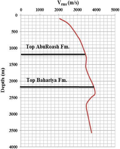

  

  V _rms for CDP 120 inline 10235

• 3. In case of dipping layers; V _rms = V _NMO.cosθ, where θ is the dip angle.

• 4. Seismic interval velocities are obtained from root-mean-square velocities using Dix (1955) equation conversion

  $$V_{\text{int}} = \left[ {\frac{{\left( {V_{{{\text{rms}}\;n}} } \right)^{2} t{}_{n} - \left( {V_{{{\text{rms}}\;\;n - 1}} } \right)^{2} t_{n - 1} }}{{t_{n} - t_{n - 1} }}} \right]^{1/2}$$

  (2)

  where V _{rms n−1}, V _{rms n} are the RMS velocities on the top and bottom of the nth layer, t _n−1 and t _n are the zero-offset travel times on the top and bottom of the nth layer.

These interval velocities (Fig. 5) depend mainly on porosity, matrix type, matrix density, fluid type, and fluid density.

Fig. 5

V _int for CDP 120 inline 10235

• 5. Interval thicknesses in m. were calculated at each CDP on reflection horizons by multiplying their two-way travel times by their interval velocities and divided by two.

  $$H_{\text{int}} { = }V_{\text{int}} \times \frac{ (\Delta T )}{ 2}$$

  (3)

  where H_int is the interval thicknesses, V _int is the interval velocity, ΔT is the two-way time difference between bottom and top of the formation.

• 6. Depths to any formation top can be calculated by summation of all overlying interval thicknesses above it.

• 7. Interval transit time (∆t) in μs/ft which is also a porosity-dependent parameter (i.e., increases with increasing porosity) can be calculated for the same CDP 120 from seismic interval velocities using:

  $$\Delta t(\upmu{\text{s}}/{\text{ft}}) = \frac{{0.3048 \times 10^{6} }}{{V_{\text{int}} }}$$

  (4)

These interval transit times are plotted in their logarithmic values against depths for each CDP as shown in (Fig. 6). This plot is very important not only for marking the onset of the abnormally high-pressure zones when the transit times are increasing with depth but also for the generation of a normal-pressure trend line that can be used for the calculation of the normal pore pressure gradient from the slope of that line opposite to the normal compaction intervals.

Fig. 6

Interval transit time for CDP 120 inline 10235

• 8. The bulk density which depends also on porosity, matrix type, matrix density, fluid type, and fluid density can be estimated either in terms of interval velocities using ENI (1999) formula:

  $$\rho_{b,i} = \rho_{\text{mat}} - 2.11\left[ {\frac{{1 - \frac{{V_{{\text{int} ,i}} }}{{V_{\text{mat}} }}}}{{1 + \frac{{V_{{\text{int} ,i}} }}{{V_{\text{mat}} }}}}} \right],$$

  (5)

  where V _int and V _mat are the interval and matrix velocities of the formation (m/s) or in terms of interval transit times using:

  $$\rho_{b,i} = \rho_{\text{mat}} - 2.11\left[ {\frac{{\Delta t_{\text{int}} - \Delta t_{\text{mat}} }}{{\Delta t_{\text{int}} + \Delta t_{f} }}} \right],$$

  (6)

  where ∆t _mat and ∆t _f are the interval transit time in the rock matrix and fluid (μs/ft).

These estimated bulk densities were compared with the measured log densities of the offset EBS-3X well as shown in (Fig. 7). A good matching was observed between the estimated and the measured well log densities for reliability of our results.

Fig. 7

Bulk densities from CDP 120 and from EBS-3X

• 1. Then the overburden pressure (P_ovb) is calculated as follows:

  $$p_{ovb} = \sum\limits_{i = 1}^{N} {\sigma_{ovb,i} } = \int {\rho_{b,i} } dD$$

  (7)

  where D is the depth of interest

• 1. Finally, pore pressure can easily be predicted from the modified Eaton’s equations (Fig. 8) as follows:

  Fig. 8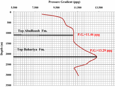

  

  Pore pressure gradient for CDP 120 along inline 10235

  $$P_{p} = \sigma_{ovb} - \left( {\sigma_{ovb} - P_{{p{\text{normal}}}} } \right)\left( {\frac{{V_{\text{observed}} }}{{V_{\text{normal}}}}}\right)^{3}$$

  (8)

  where V _observed and V _normal are the observed interval velocity of the abnormally compacted and the normally compacted zones, respectively.

Results and interpretation

Totally, 154 CDPs along 28 seismic lines were examined in the study area. For pore pressure prediction, 84 CDPs were selected on 14 inline seismic sections and 70 CDPs selected on 14 crosslines. Wide variability and great contrasts of acoustic impedances are observed on the reflection horizons of this section which are indicated by clear reflections with good amplitude data quality.

Tectonic activities are represented by several normal faults along this section causing more changes in the position (depth) of each formation relative to one another and providing several horsts (high structural features) and graben structures.

When fault elements dissect a permeable layer, a connection can be developed between shallower part (up thrown side) with the deeper one (downthrown side) that, in turn, will provide vertical fluid flow path and the pressure transfer from the higher-pressured part (deeper) to the shallower part until the two pressures are equalized. Then the shallower part will have a higher pore pressure than it should as a result of two natural causes: faulting and repressuring.

However, in case of a permeable layer (sand) surrounded by impermeable barriers (shale or carbonate seal) on all sides and intact uplifting to a shallower depth, the pore pressure within this layer will be the same anywhere within its boundaries, and it is also the same before and after uplifting, while the pore pressure gradient in the uplifted part of this layer increases after uplifting because it is now at a shallower depth relative to the surface and will require heavier mud weight to drill.

Root-mean-square velocities represented by 2D cross-sectional RMS velocity model for all CDPs along that inline seismic section 10235 is illustrated in (Fig. 9). In normal situations, the velocity increases with depth. However, two velocity reversal zones were observed with lower values for most of CDPs on that seismic line at depth intervals of 1417–1817 m and 2373–2491 m which are correlated with Abu Roash members “A” to “E” and Bahariya Formation, respectively, as shown in V _int relation with depth (Fig. 10). These two zones of lower velocities are separated from each other by higher velocity carbonates of Abu Roash member “F”.

Fig. 9

2D cross-sectional RMS velocity model for all CDPs along inline 10235

Fig. 10

Interval velocity for 6 CDPs along inline 10235

The 2D cross-sectional V _int model (Fig. 11) indicates that these two low-velocity anomalies are characterized by lower bulk densities as shown in (Fig. 12), and therefore, they are under compacted zones. Overburden pressures were calculated from the integration of these bulk densities multiplied by their corresponding thicknesses.

Fig. 11

2D interval velocity model along inline 10235

Fig. 12

2D bulk density model along inline 10235

Finally, the pore pressures were calculated along that inline 10235 using the modified Eaton’s Eq. (8) in lb/gal (ppg) and confirmed that these two zones of lower interval velocities are overpressured zones as shown in (Fig. 13), and 2D pore pressure gradient model for this line is shown in (Fig. 14). It is possible to predict fluid (water, oil, gas) producing reservoirs in these abnormal formation pressure regions.

Fig. 13

Pore pressure gradient along inline 10235

Fig. 14

2D pore pressure gradient model along inline 10235

It can be concluded from inline 10235 that the pore pressures and the pore pressure gradients of the first zone start increasing gradually from normal-pressure trendline in the shallower parts to a transition zone in a depth of about 1417 m (top Abu Roash member “A”), then to an abnormal pressure region that cwontinues till a depth of 1817 m base of this member attaining maximum values of pore pressure about 4407 psi and pore pressure gradient of 11.46 ppg or 0.59 psi/ft, while the second abnormal pressure zone starts at a depth of about 2373 m from top Bahariya Formation and continues up to its base and sometimes till Kharita Formation with maximum pore pressure of 5659 psi and pore pressure gradient of 13.292 or 0.69 psi/ft.

The same analysis was carried out for the rest of inline seismic sections in the NE–SW direction and also for all crosslines in the NW–SE direction. These relations verify and prove that Abu Roash members “A” to “F” and Bahariya till Kharita Formations have abnormal pressure zones, and they might be oil producing reservoirs in Beni Suef Field area as it was confirmed later while drilling that Abu Roash A, E, and “G” members and Bahariya and Kharita Formations are really oil producing reservoirs.

For dynamic equilibrium during drilling, it is necessary to equalize (balance) the hydrostatic pressures with those predicted abnormal pore pressures and gradients, to avoid any drilling problem. The abnormal pore pressures at these two zones can now be considered as hydrostatic pressures that can be used for the calculation of the compensated mud weights as follows: mud weight (ppg) = hydrostatic pressure (psi)/0.052 × h (ft). The required heavier mud weight to drill is 11.98 ppg for Abu Roash and 13.8 ppg for Bahariya Formation.

Rouchet (1981) mentioned that the migration of oil seems to involve two processes: (1) lateral transfer, by channeling into the more coarsely microporous layers of the source rock, from the oil generation site toward the geologic structure or lower-pressured zone; and (2) vertical transfer from the source rock to reservoir by the opening or reopening of vertical fractures in the few areas, such as structural tops, where the least compressive stress is equal to the pore pressure, and where the capillary pressure increment of oil in the microporosity exceeds the tensile strength of the rock.

Migration processes depend mainly upon the tectonic activities which have occurred through fault elements and uplifting in the study area. The migration of the generated oil starts from basins to ridges and high structural features laterally, diagonally, or vertically. The migration paths are primarily depending on the interconnected pore channel ways and secondly on the open fracture system (faulting). The fluids are distributed outward from the higher pressures and higher pressure gradients to the lowest ones, and the fluid flow paths are oriented perpendicular to the isopressure and isopressure gradient contour lines pointing toward the parts of the lowest pressure gradient (Dahlberg 1982).

Finally, we had to establish pore pressure gradient maps (Figs. 15, 16) within these two promising zones for Abu Roash and Bahariya Formations to have a look at the areal distribution of the pore pressure gradients within them and to indicate the directions of the horizontal fluid flows (migration paths) by black arrows to propose prospects with little drilling problems.

Fig. 15

Pore pressure gradient map within Abu Roash Formation

Fig. 16

Pore pressure gradient map within Bahariya Formation

Pore pressure gradient map within Abu Roash Formation (Fig. 15) exhibits the locations of both higher and lower pressure gradients. Higher-pressure-gradient anomalies occupy the southwestern, northeastern, and eastern parts attaining a maximum value of 12.5 ppg (0.66 psi/ft), while the southern and northwestern corners represent the lower-pressure-gradient anomalies reach 8 ppg (0.41 psi/ft).Three possible locations (P1, P2, and P3) are proposed within the Abu Roash Formation (Fig. 15) as proposed prospects based on the pre-drill pore pressure prediction, seismic interpretation, and geological information due to their lower pore pressures, lower pore pressure gradients, and seismic structurally high.

Pore pressure gradient map within Bahariya Formation (Fig. 16) exhibits the locations of both higher and lower pressure gradients. Higher-pressure-gradient anomalies occupy the southeastern, central, northeastern, and western parts attaining a maximum value of 13.8 ppg (0.72 psi/ft), while the southwestern and northwestern corners represent the lower-pressure-gradient anomalies reach 10 ppg (0.52 psi/ft). Four possible locations (P1, P2, P3, and P4) are proposed within the Bahariya Formation (Fig. 16) as proposed prospects based on the pre-drill pore pressure prediction, seismic interpretation and geological information due to their lower pore pressures, lower pore pressure gradients, and seismic structurally highs.

Finally, it could be concluded from Abu Roash and Bahariya pore pressure gradient maps that they indicate:

• 1. The proposed locations of abnormally high pore pressure and gradient anomalies,

• 2. The expected depths of possible kicks at these anomalies,

• 3. The expected faster penetration rates at these abnormal pressure anomalies,

• 4. The heavier mud weight that is required and recommended to drill (13.8 ppg),

• 5. The direction of the possible horizontal fluid flow (migration paths) as indicated by black arrows,

• 6. The proposed locations of the new prospects (lowest pressure and lower pressure gradient).

We can correlate our prediction for the new prospects from Abu Roash and Bahariya Formations pressure gradient maps with the depth structure maps on the tops of these formations. Figure 17 shows the structure features affecting Abu Roash Formation, which are represented by several faulted folds. The predicted prospect locations of the lower pressure zones on (Fig. 15) will occur on structurally highs on (Fig. 17).

Fig. 17

Depth structural contour map on the top of Abu Roash Member(A) Formation

Conclusions

Numerous problems such as dangerous well kicks, lost circulation, blowouts, stuck pipe, excessive costs, and borehole instability may arise while drilling, if pore pressure is not predicted before drilling. Pre-drill pore pressure prediction in the form of velocity-to-pressure transform has been carried out utilizing surface seismic survey data. Estimated bulk densities from seismic interval velocities at each seismic line were compared with the measured densities of the closest well. Good matching has been observed between the estimated and measured densities for reliability of our pressure results. Overburden pressure at any interested depth was calculated from summation products of interval bulk densities and their corresponding thicknesses of all layers overlying that depth. Pore pressures were predicted from subtraction of the effective stresses (skeleton pressure, matrix stress) in terms of normal and observed interval velocities from overburden pressures using the modified Eaton’s equation method.

Two velocity reversal zones (low-velocity layers) for all of the 154 CDPs along 28 seismic lines separated from each other by higher velocity carbonates of Abu Roash member “F” were observed and correlated to Abu Roash members “A” to “E” and Bahariya Formation. Skeleton pressures as well as elastic parameters are decreased on the expense of increasing pore pressures in these abnormal pressure zones due to their decrease in interval velocities and densities.

Knowledge of pore pressure is very important in deciding the drilling mud weight to be used. Drilling mud in the borehole creates hydrostatic head to balance the formation pressure during drilling. For dynamic equilibrium during drilling, it is necessary to equalize (balance) the hydrostatic pressures with those predicted abnormal pore pressures and gradients, to avoid drilling problems. The abnormal pore pressures at these two zones can now be considered as hydrostatic pressures that can be used for the calculation of the compensated equivalent mud weights. The heavier mud weight that are required and recommended to drill is 13.8 ppg. It is possible to predict the fluid (water, oil, gas) producing reservoirs in these abnormal pore pressure zones.

Moreover, pore pressure gradient maps were established for these two abnormal pressure zones indicating (1) their areal locations and distributions, (2) possible kicks starting from their tops, (3) expected faster rate of penetration, (4) heavier mud weight that is required and recommended to drill (13.8 ppg), (5) direction of possible horizontal fluid flow (migration paths), (6) proposed locations of prospects of the lowest pore pressures and pore pressure gradients with least drilling problems.

References

Babu S, Sircar A (2011) A comparative study of predicted and actual pore pressures in Tripura, India. J Pet Technol Altern Fuels 2(9):150–160
Bourgoyne AT, Millheim KK, Chenevert ME, Young FS (1991) Applied drilling engineering, revised 2nd printing, Society of Petroleum Engineering, Richardson, TX, pp 246–667
Bowers GL (1995) Pore pressure estimation from velocity data: accounting for overpressure mechanisms besides under compaction. SPE Drill Completion 10(2):89–95
Brahma J, Sircar A, Karmakar G (2013) Pre-drill pore pressure prediction using seismic velocities data on flank and synclinal part of Atharamura anticline in the Eastern Tripura, India. J Pet Explor Prod Technol 3(2):93–103
Carcione JM, Helle HB (2002) Rock physics of geopressure and prediction of abnormal pore fluid pressures using seismic data. CSEG Rec 9:8–32
Chopra S, Huffman A (2006) Velocity determination for pore pressure prediction. CSEG Rec 3:28–46
Dahlberg EC (1982) Applied hydrodynamics in petroleum exploration. Springer, New York, p 155
Dix CH (1955) Seismic velocities from surface measurements. Geophysics 20:68–86
Dutta NC, Ray A (2002) Geopressure detection using seismic data: current status and the road ahead. Geophysics 67(6):2012–2041
Dvorkin J, Mavko G, Nur A (1999) Overpressure detection from compression and shear-wave data. GRL 26:3417–3420
Eaton BA (1975) The equation for geopressure prediction from well logs. SPE of AIME, Dallas, TX, SPE 5544 September 28–October 1, Dallas, pp 1–11
Egyptian General Petroleum Corporation (1996) Gulf of Suez Oil Fields: EGPC. Special publication, Egypt
ENI SPA (1999) Overpressure evaluation manual, company manual, pp 141–170
Fertl WH (1976) Abnormal formation pressures. Elsevier Scientific Publishing Company, Amsterdam, p 424
Gardner GHF, Gardner LW, Gregory AR (1974) Formation velocity and density—the diagnostic basis for stratigraphic traps. Geophysics 39:770–780
Kan TK, Kisdonik B, West CL (1999) 3-D geopressure analysis in the deepwater Gulf of Mexico. Lead Edge 18(4):502–508
Lu XX, Jiao WW, Zhou XY, Li JJ, Yu HF, Yang N (2009) Paleozoic carbonate hydrocarbonaccumulation zones in Tazhong Uplift, Tarim Basin, western China. Energy Explor Exploit 27(2):69–90
Rieke HH III, Chilingarian GV (1974) Compaction of argillaceous sediments. Elsevier, Amsterdam, p 424
Rouchet JD (1981) Stress fields, a key to oil migration. Bull AAPG 65:74–85
Rubey WW (1927) Effect of gravitational compaction on the structure of sedimentary rocks. AABG Bull 11:621–632
Sayers CM, Johnson GM, Denyer G (2002) Pre-drill pore-pressure prediction using seismic data. Geophysics 67(4):1286–1292
Schlumberger (1984) Well evaluation conference, Egypt, Ch. 1: In Geology of Egypt, 64 p
Sundaram KM, Jain R (2008) Eaton’s equation and compaction—a study. In: 7th International conference & exposition on petroleum geophysics, SPG, pp 311–317
Swarbick RE, Huffman AR, Bowers GL (1999) Pressure regimes in sedimentary basins and their prediction. Lead Edge 18:511–513
Author information
Authors and Affiliations
Corresponding author
Rights and permissions
Open Access This article is distributed under the terms of the Creative Commons Attribution 4.0 International License (http://creativecommons.org/licenses/by/4.0/), which permits unrestricted use, distribution, and reproduction in any medium, provided you give appropriate credit to the original author(s) and the source, provide a link to the Creative Commons license, and indicate if changes were made.
About this article
Cite this article
El-Werr, A., Shebl, A., El-Rawy, A. et al. Pre-drill pore pressure prediction using seismic velocities for prospect areas at Beni Suef Oil Field, Western Desert, Egypt. J Petrol Explor Prod Technol 7, 1011–1021 (2017). https://doi.org/10.1007/s13202-017-0359-6
Received:
Accepted:
Published:
Issue Date:
DOI: https://doi.org/10.1007/s13202-017-0359-6