Palaeoclimatic models - predicted changes in the potential Neogene distribution patterns of Phlebotomus similis and Phlebotomus sergenti (Insecta: Diptera: Psychodidae)

Abstract

Former studies proposed that the speciation of the subgenus Paraphlebotomus happened in the Neogene Epoch in the circum-Mediterranean region due to the geographical segregation effect of the former Paratethys Sea. It was aimed to study whether the modelled Neogene ranges of Phlebotomus sergenti and Phlebotomus similis support or contradict this barrier role of the Paratethys in the speciation of Paraphlebotomus sandfly. For this purpose, the potential Neogene geographical ranges of Phlebotomus sergenti and Phlebotomus similis were modelled based on the present climatic requirements of the taxa. The Miocene models do not support the circum-Paratethyan migration of the ancestor of Phlebotomus similis. In general, Phlebotomus similis shows a low affinity to the North Paratethyan shorelines during the entire Miocene epoch. The only exceptions are the Tortonian and early Messinian periods when the climatic conditions could be suitable for Phlebotomus similis in the North Paratethyan shorelines. It was found that neither the modelled late Miocene, Pliocene nor the mid-Pleistocene period distributions of Phlebotomus sergenti and Phlebotomus similis shows notable differences in the suitability values in the Balkans and the Middle East. It is most plausible that the divergence of the Phlebotomus similis and its relatives was related to the tectonic subsidence of the Hellene Orogenic Belt and Phlebotomus similis specialised in the Balkan Peninsula and the present-day North Pontic area during the middle-late Miocene epoch. The Messinian desiccations of the Mediterranean Basin and the Zanclean re-flood caused the migration, but not the speciation of Phlebotomus similis and its sister taxa.

Introduction

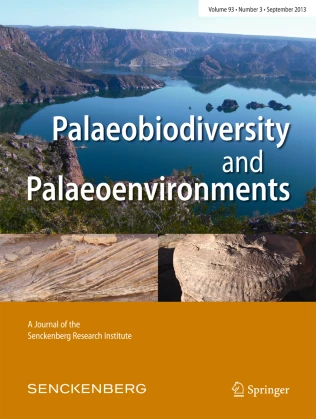
As members of the Mediterranean fauna, the Mediterranean sandfly species are the vectors of several Phleboviruses and Leishmania parasites which are the causative agents of serious veterinary and human diseases. Leishmaniasis is an emerging epidemiological hazard in Europe (Ready 2010). Sandfly-borne diseases not only mean significant health risks, but they also impose a notable economic burden on society. For example, only in Italy, the direct costs for hospital admissions related to human leishmaniasis were between 1,637 and 1,370 thousand euro per year in the period 1999–2003 (Mannocci et al. 2007). Sandfly-borne diseases also cause great veterinary expenditures in Europe. In Spain, a study revealed that up to 13–20% of dogs can be infected with Leishmania infantum Nicolle, 1908 in the thermo-Mediterranean and meso-Mediterranean territories (Martín-Sánchez et al. 2009). These dogs also serve as the source of zoonotic leishmaniasis for humans (Quinnell and Courtenay 2009). The members of the Phlebotomine sandfly subgenus Paraphlebotomus are typical members of the Mediterranean entomofauna. Phlebotomus (Paraphlebotomus) sergenti Parrot, 1917, the main and only proven vector of Leishmania tropica Wright, 1903 among the members of the subgenus Paraphlebotomus (Depaquit et al. 2002), presently has a circum-Mediterranean range, including North Africa, the Hispanian Peninsula, South France, Sicily, the Balkans, the Greek islands, Asia Minor, Levant and the Caucasus (ECDC 2020). In contrast, Phlebotomus (Paraphlebotomus) similis Perfiliev, 1963, the second, suspected vector of L. tropica within the subgenus Paraphlebotomus (Antoniou et al. 2013), only can be found in the Balkans, the Greek islands and Asia Minor (ECDC 2020).

There is growing interest to understand the influences of past climate changes on vector arthropod species for the better prediction of the possible effects of the anthropogenic climate change (e.g. Perrotey et al. 2005). It seems that the Neogene period played an important role in the speciation and the determination of the present climatic requirements of certain members of the Mediterranean arthropod fauna (e.g. Esseghir et al. 1997, 2000; Depaquit et al. 2000; Trájer et al. 2018a). The Neogene palaeogeography of the Tethys and the Paratethys and the Pliocene-Pleistocene climatic fluctuations strongly influenced the recent area and the primary diversification of several circum-Mediterranean faunae (Oosterbroek and Arntzen 1992). This is rooted in the parallel cooling of the Earth from the turn of the Oligocene and Miocene epochs (McKay et al. 2016) and the complex geographical history of the circum-Mediterranean area which was strongly affected by the tectonic motions of Africa, Europe and several minor landmasses during the Alpine orogenesis (Rosenbaum et al. 2002). The opening of the Provencal Basin in the Oligocene, and the extension of the Pannonian Basin during the Miocene, fundamentally transformed the geography of the entire Mediterranean area (Carminati and Doglioni 2005; Balázs et al. 2016). In the early Miocene epoch (ca. 20 Ma), the Paratethys was well-connected with the Mediterranean (the Tethys) Sea and the Indian Ocean (Steininger and Rögl 1984). The geography of the seaways and the level of connectivity between the two large seas dramatically changed in the Neogene Epoch (Popov et al. 2006). In the middle Miocene era, the Dinaric-Hellenic Orogenic Arc formed a land bridge between Asia and the land of the present-day Balkan Peninsula (Jones et al. 1992). At that time, the fauna of the Balkan and the Middle East was separated from continental Europe due to the Central Paratethys Basin and the Slovenian corridor (Fodor et al. 1998). In the early Serravallian (ca. 13 Ma), the waters of the Central Paratethys and the Mediterranean Sea communicated with each other (Bartol et al. 2014) which caused the alternating level of separation of the landmasses of the Central Paratethys, the Middle East and the European Continent. In the latest Miocene period, the Messinian, the Tethys repeatedly desiccated and flooded again, which allowed the terrestrial fauna to migrate to the islands of the Mediterranean (Hsü 1974). Generally, this event is thought to be a milestone in the speciation of the Mediterranean sandfly species (e.g. Kasap et al. 2015). In the Pliocene epoch, the former Paratethys Sea was divided into several inland seas, which meant the disappearance of the former geographical barrier between the Middle East and Europe (Popov et al. 2006) (Fig. 1).

Fig. 1

The geography of the wider Mediterranean area in the Sarmatian (late Serravallian), ca. 13–14 Ma

It is very plausible that the origin of the different actual ranges of the species goes back at least to the first part of the Neogene epoch (Esseghir et al. 2000; Trájer et al. 2018a). The colonisation of the Mediterranean Basin by the subgenus Paraphlebotomus may have occurred in the Miocene period (Depaquit et al. 1998). The extant Mediterranean Paraphlebotomus species had a common Asiatic ancestor and the centre of dispersion of the genus Paraphlebotomus might have been somewhere in South Asia (Depaquit et al. 2000; Alten 2010). Two migration routes were proposed, one, north of the Paratethys Sea and another south of the Paratethys and Tethys Seas. The first route was postulated as the cause for the isolation of Ph. similis, the second route may have contributed to the speciation of Ph. sergenti (Depaquit et al. 1998). Based on the internal transcribed spacer 2 (ITS2) sequences of 12 sandfly populations from 10 countries, Depaquit et al. (2002) and Alten (2010) found that the ancestor of Ph. similis originally colonised the Caucasus, the Crimean and the Balkan Peninsulas, including the Aegean islands and the western part of Asia Minor. In contrast, it was hypothesised that Ph. sergenti followed an east-west Asiatic migration route through the landmasses between the former Tethys and the Paratethys Seas in Asia. The species colonised North Africa and migrated to the Iberian Peninsula passing through the formerly dryland Betic Bridge (Léger and Depaquit 2002; Alten 2010). Esseghir et al. (2000) and Trájer et al. (2018A) found that the ecological niches and the climatic distribution limiting values of the extant Mediterranean Phlebotomus species are the consequence of the climatic and geographical events of the Neogene era. While the present eastern distribution area of Ph. sergenti and Ph. similis is highly similar, the distribution limiting values of the two species are somewhat different. This may be due to the fact that the two species developed in different areas and climate zones (Trájer et al. 2018a). Based on the proposed North Paratethyan former range of Ph. similis, it can be hypothesised that this species should be more cold-tolerant than Ph. sergenti, which might rather have kept the climatic needs of the common ancestor of the two taxa. Because the retreat of the Central Paratethys Sea occurred in the Pliocene Period, this era may be the time when the geographical barrier between the two species disappeared. If the zoogeographic hypothesis outlined above is true, the modelled distributions of the ancestors of the two species had to be different around the Paratethys realm in the Pliocene era.

Aims

It was aimed to test the hypothesis that Ph. similis originally evolved in the northern, Ph. sergenti on the southern coastal areas of the Paratethys. To investigate the hypothesis, it was aimed to model the middle Pliocene and middle Pleistocene potential distribution of Ph. similis and Ph. sergenti, the climatic suitability of the North Pontic area for Ph. similis during the Miocene epoch and the suitability of the East Mediterranean and Paratethys area for the two species in the late Miocene (Tortonian) era. The approach was based on the principle of actualism, using the present climatic requirements of the species for Europe and the Middle Paratethys region. A specific aim was to examine whether Ph. similis could have more affinity to the North Paratethys region than its sister taxa or not. If the proposed difference in the potential ranges cannot be confirmed, the modification of the speciation theory of the two species in correspondence with the previous phylogenetic results of the literature is required.

Materials and methods

The logical framework and methodological considerations of the study

The following work plan has been identified:

• 1) According to the previously published Paraphlebotomus speciation theories, the North Pontic area, as the part of the northern coastline region of the East Paratethys Basin, should have a prominent role in the speciation of Ph. similis (Depaquit 1998, 2000, 2002). Due to geographical considerations, this area could also be the source of the southward migration of the species further to their current in Southeast Europe and Asia Minor in the Pliocene, when the remains of the Paratethys became individual seas. Due to these considerations, the suitability of the North Pontic area was modelled for the entire Miocene epoch to determine whether this area could be the speciation centre and migration route of the species or not (model A).

• 2) Because the Tortonian-early Messinian era could be the last period when the speciation of Paraphlebotomus occurred (see the ‘Discussion’ section for the explanation), this period which is called ‘Pannonian’ in the Central Paratethyan regional stratigraphy was considered separately in the modelling (model B).

• 3) The mid-Pliocene and mid-Pleistocene potential distribution of Ph. sergenti and Ph. similis were modelled to investigate the similarities and differences of the distribution of the two species around the Central and East Paratethys area, after the disintegration into sub-basins of the formerly unified Paratethys Sea. This step is important to investigate whether immediately after the Pliocene disappearance of the unified basin Ph. similis had a better climatic affinity to the North Paratethys area compared to Ph. sergenti or not because this time was the time when the geographical segregation of the Ph. similis and its sister taxa ended (model C).

It is a basic methodological difficulty that if we look back to the ages of earth history, we have no statistically significant amount of occurrence data which could provide the basis for the determination of distribution limiting climatic values. Fossil Phlebotominae species can be found in the fossil record, e.g. †Phlebotomites aphoe Stebner et al., 2015, †Phlebotomites burmaticus Malak et al., 2013, †Phlebotomites grimaldii Malak et al., 2013, †Phlebotomus khludae Stebner et al., 2015, †Phlebotomites neli Malak et al., 2013 and †Phlebotomus vetus Stebner et al., 2015 from the Burmese amber (Stebner et al. 2015), which is in a Cenomanian (99.7 to 94.3 Ma old) terrestrial amber in Myanmar or †Phlebotomus pungens Loew, 1845 from a single Quaternary occurrence of Tanzania (Ross 2018). This fossil record is so poor that the known occurrence data of extinct species is completely useless for modelling purposes. Naturally, it cannot be set that the ecological (e.g. climatic) requirements of the ancestors of the extant species did not change in the Neogene period and were equal to the ecological demands of the present species. Although the environmental requirements of the ancestors of the recent sandfly species are not known, the climatic demands of the extant species can provide the basis for the examination of the Miocene-Pliocene-Middle Pleistocene distribution of the taxa. Climate determines the range of sandfly taxa, and it is possible that climatic variables also strongly influenced the past occurrences of the species. As it was described in the ‘Introduction’, sandfly species appear to be quite conservative in their environmental demands, and it is possible that the environmental requirements of the Mediterranean sandfly were determined by the climatic effects and geographic conditions of the Neogene period (Esseghir et al. 2000; Trájer et al. 2018a). It is also known that the distribution limiting climatic values of Ph. sergenti, which is one of the closest living relatives of Ph. similis, is very similar to the previous species (Table 1; Trájer et al. 2013) even though the divergence of the two species should occur in the mid-Miocene epoch, before the disappearance of the Paratethys Sea (Depaquit et al. 2002). This indicates that the common ancestors of the two species may have had similar climatic needs, and that, throughout their history, similar climatic needs have been maintained by the sister species. Based on the above-described considerations, although with certain restrictions and cautions, the present climatic requirements of the two species can be used as the basis of the modelling of the former distribution of their ancestors.

Table 1 The ages of the fossil palaeoflora sites in the palaeoclimatic reconstruction of Syabryaj et al. (2007) expressed in regional and global stratigraphic units; *local, southern Ukrainian stratigraphic unit, **Paratethyian stratigraphic unit, ***global stratigraphic unit

Although Phlebotomus (Paraphlebotomus) jacusieli Theodor, 1947 has a slightly closer phylogenetic relationship to Ph. similis than Ph. sergenti (Depaquit et al. 2002), the past occurrences of Ph. jacusieli were not modelled in the present study. This is partly because of the previously established speciation models, which described the parallel development of Ph. similis and Ph. sergenti. On the other hand, the climatic requirements of Ph. jacusiely are not known sufficiently. For these reasons, in this study, primarily the speciation of Ph. similis in the Miocene epoch, and in parallel, the potential former distribution of Ph. sergenti, was studied in the mid-Pliocene and the mid-Pleistocene periods.

The climatic extrema used in the study

To create the distribution models, the occurrence limiting climatic variables of Trájer et al. (2013) were used. The authors performed their analyses based on the distribution data of the European Centre for Disease Prevention and Control. This uses several occurrence categories, like ‘present’ and ‘introduced’. Trájer et al. (2013) handled only the ‘present’ category data as positive areas for permanent occurrence. For the explanation of the employed distribution limiting values, see the model identification subchapters.

Sources of the used climate models

The Miocene climate models used in this study were based on the determination of the differences between the past and the present bioclimatic values. These regional climate models were created by the modification of the reference period’s climate model using the difference values from the present climatic conditions in the case of each climatic factor. To maintain the validity and reliability of the developed models, the georeferenced models were only specified for the northern area of the Black Sea. The palaeoclimatic data of the North Pontic region was gained from Syabryaj et al. (2007). Because the reconstructed values were not directly used in modelling and the utilisation of climatic reconstructions for modelling purposes cannot be distinguished from the explanation of the development of model environment A, see the detailed explanation of this climate model in the related subchapter ‘Model identification of model environment A’. The model environment B covers the Tortonian period, which is equal to the Paratethyan regional stratigraphy unit Pannonian period sensu stricto. The Pannonian (Tortonian) climate model was based on the palaeoclimatic reconstruction of Bruch et al. (2006). In model environment C, previously developed, global-scale climate models were used. The georeferenced climate data were taken from WorldClim database. The WorldClim version 2 (Fick and Hijmans 2017) has average monthly climate data for minimum, mean and maximum temperature and for precipitation for 1970–2000, which reference period was used for comparison and verification purposes. For modelling the past conditions, cold and warm period models of the mid-Pliocene epoch were used. The cold period model was constructed by Dolan et al. (2015) and it represents the M2 mid-Pliocene warm period 3.264–3.025 Ma. The warm period model was constructed by Hill (2015) and represents the middle Pliocene glaciation stage 3.3 Ma (more exactly: 3.29–3.42 Ma) in the Piacenzian. The MIS19 mid-Pleistocene period’s model (ca. 787 ka) was constructed by Brown et al. (2018).

Topographical reconstructions

Naturally, the sea level model of the Miocene epoch can only be indicative. It cannot be the object of a palaeobiogeographic study to exactly reconstruct the past fluctuations of the global and the Paratethyan sea levels or the tectonic history of the area. What is important in this aspect is that the Mediterranean terranes approximately reached their present positions at the turn of the Oligocene and Miocene epochs in the Central Paratethys (Kvaček et al. 2006; Kováč et al. 2017) creating geographic patterns that were similar to the present conditions in the central basins of the sea. For a general approximation, it can be accepted that about a plus 60-m enhancement of the present sea level conditions can be used to indicate the former seashore patterns. The geological reconstructions show very similar shorelines in the Paratethys that was used in the present study (compare with the reconstructions of Popov et al. 2006; Palcu et al. 2019). The approximate shoreline patterns of the Pannonian Lake in about 10 Ma in model C was based on Magyar et al. (1999).

Identification of model environment A

The first model environment (model environment A) was performed to model the Miocene potential distribution of Ph. similis, using the climatic requirements of the extant species. Since available, high-resolution climate models were not available for the North Pontic area, which is identical to the former northwester seashore region of the East Paratethys, climate models were developed based on the modifications of the reference climate maps according to the palaeoclimatic data of Syabryaj et al. (2007). The authors investigated the fossil Miocene vegetation of South Ukraine. Because the Miocene strata of Ukraine belong to the Central and Eastern Paratethys, this region is the target area of the speciation of Ph. similis according to the theory of Depaquit (1998) and Alten (2010). Using the Coexistence Approach (Mosbrugger and Utescher 1997), Syabryaj et al. (2007) reconstructed the Miocene palaeoclimate of the region for the Aquitanian, Burdigalian, Tarkhanian (lower-middle Langhian), Badenian (Langhian and lower Serravallian), Sarmatian (upper Serravallian), Maeotian (upper Tortonian-lower Messinian) and the Pontian (upper Messinian) ages (for the explanation of the periods see Table 1). The reconstruction of Syabryaj et al. (2007) does not cover the period of the Pannonian regional stratigraphic unit (the Tortonian).

The Coexistence Approach concept is based on the distribution of limiting values of the closest extant relatives of the fossil taxa. This method can be accepted for the Neogene period due to the time proximity; if the fossil record is treated with caution, many fossil taxa are involved, and the climatic demands of the living taxa are analysed with appropriate statistical tools (Mosbrugger and Utescher 1997). Syabryaj et al. (2007) investigated microflora and concerned three thermal and four precipitation climate variables: the mean annual temperature, the cold month mean temperature, the warm month mean temperature, the mean annual precipitation, the precipitation in the warmest month, the precipitation in the driest month and the precipitation in the wettest month. Because Syabryaj et al. (2007) used classic bioclimatic categories, some georeferenced bioclimatic variables of the PaleoClim database could easily correspond, others not. To increase the number of variables, two derived variables, i.e. the annual monthly average and July Thornthwaite agrometeorological aridity indices (sing. abbr.: TAI), were introduced which values directly can be derived from the precipitation and temperature values (Kemp, 2002). The common formula of the TAI index is the following:

$$ \mathrm{TAI}=1.65\times {\frac{P}{T+12.2}}^{\left(\frac{10}{9}\right)} $$

where TAI is the Thornthwaite agrometeorological aridity index in millimetres per °C, P is the monthly precipitation sum in millimetres and T is the monthly mean temperature in °C.

In the present study, the annual mean values of the climatic variables and the July values were used. The use of the aridity index is justified by the act that sandfly species are highly sensitive to the combination of strong solar radiation and atmospheric drought (Elnaiem et al. 1998; Trájer et al. 2018b).

The used climatic variables were as follows: the lower and upper limits of the annual mean of the temperature (Tam; °C; Bioclim1), the lower and upper limits of the January mean temperature (T1mmin,max, °C); the lower and upper limits of the July mean temperature (T7mmin,max, °C); the lower and upper limits of the annual precipitation sum (Paslimit.min,max, mm; Bioclim12); the July precipitation sum (P7slimit.min,max, mm); the lower and upper limits of the annual mean monthly Thornthwaite agrometeorological aridity index (TAIalimit.min,max, mm°C⁻¹); the lower and upper limits of the July Thornthwaite agrometeorological aridity index (TAI7limit.min,max, mm°C⁻¹). Supplementary Table 1 shows the calibration of the climate models.

This means 7 × 2 bioclimatic factors in the model, in the case of both species, that is an acceptable number for distribution modelling purposes. For the numerical modelling of the potential distribution areas of species, these 7 × 2 extrema of climatic factors were used. Similarly, in the Pliocene-Pleistocene models, the modelling was based on the binary logic of the Boolean algebra that means that should indicate that the mathematical formalism of the deterministic unit step functions should also be similar:

$$ {\displaystyle \begin{array}{c}1(Tam)=\left\{\begin{array}{c}0\kern1.25em if\kern1.25em {Tam}_{limi\mathrm{t}.\mathit{\min}}> Tam>{Tam}_{limi t.\mathit{\max}}\\ {}1\kern1.25em if\kern1.5em {Tam}_{limi t.\mathit{\min}}\le Tam\le {Tam}_{limi t.\mathit{\max}}\end{array}\right.\\ {}1(T1m)=\left\{\begin{array}{c}0\kern1.25em if\kern1.25em T1{m}_{limi t.\mathit{\min}}>T1m>T1{m}_{limi t.\mathit{\max}}\\ {}1\kern1.25em if\kern1.5em T1{m}_{limi t.\mathit{\min}}\le T1m\le T1{m}_{limi t.\mathit{\max}}\end{array}\right.\\ {}\begin{array}{c}1(T7m)=\left\{\begin{array}{c}0\kern1.25em if\kern1.25em T7{m}_{limi t.\mathit{\min}}>T7m>T7{m}_{limi t.\mathit{\max}}\\ {}1\kern1.25em if\kern1.5em T7{m}_{limi t.\mathit{\min}}\le T7m\le T7{m}_{limi t.\mathit{\max}}\end{array}\right.\\ {}1(Pas)=\left\{\begin{array}{c}0\kern1.25em if\kern1.25em {Pas}_{limi t.\mathit{\min}}> Pas>{Pas}_{limi t.\mathit{\max}}\\ {}1\kern1.25em if\kern1.5em P{as}_{limi t.\mathit{\min}}\le Pas\le {Pas}_{limi t.\mathit{\max}}\end{array}\right.\\ {}\begin{array}{c}1(P7s)=\left\{\begin{array}{c}0\kern1.25em if\kern1.25em P7{s}_{limi t.\mathit{\min}}>P7s>P7{s}_{limi t.\mathit{\max}}\\ {}1\kern1.25em if\kern1.5em P7{s}_{limi t.\mathit{\min}}\le P7s\le P7{s}_{limi t.\mathit{\max}}\end{array}\right.\\ {}1\left( TAI a\right)=\left\{\begin{array}{c}0\kern1.25em if\kern1.25em {TAIa}_{limi t.\mathit{\min}}> TAI a>{TAIa}_{limi t.\mathit{\max}}\\ {}1\kern1.25em \mathrm{i}f\kern1.5em {TAIa}_{limi t.\mathit{\min}}\le TAI a\le {TAIa}_{limi t.\mathit{\max}}\end{array}\right.\\ {}1(TAI7)=\left\{\begin{array}{c}0\kern1.25em if\kern1.25em TAI{7}_{limi t.\mathit{\min}}> TAI7> TAI{7}_{limi t.\mathit{\max}}\\ {}1\kern1.25em if\kern1.5em TAI{7}_{limi t.\mathit{\min}}\le TAI7\le TAI{7}_{limi t.\mathit{\max}}\end{array}\right.\end{array}\end{array}\end{array}} $$

where Tam represents the lower and upper limits of the annual mean temperature, T1m is the georeferenced climate model data of the lower and upper limits of January mean temperature and T7m is the georeferenced climate model data of the lower and upper limits of July mean temperature. Pas represents the georeferenced climate model data of the annual precipitation sum and P7s is the georeferenced climate model data of the July precipitation sum. TAIa is the annual mean monthly Thornthwaite agrometeorological aridity index, and TAI7 is the July Thornthwaite agrometeorological aridity index.

The potential areas can be determined according to the following mathematical formalism:

$$ A\left( Tam;T1m;T7m; Tmc; Pas; Pswm; Psdm; Pscq\right)= Tam\bigcap T1m\bigcap T7m\bigcap Pas\bigcap P7s\bigcap TAI a\bigcap TAI7 $$

where A(Tam;T1m;T7m; Pas; P7s;TAIa;TAI7) shows the potential distribution area of the given species, which contains the remaining areas after taking into consideration the temperature and precipitation limitations.

Identification of model environment B

This model environment was established to investigate the potential range of Ph. sergenti and Ph. similis during the Pannonian (Tortonian) era. The late Miocene Pannonian age model was based on the palaeoclimatic reconstruction of Bruch et al. (2006). The Pannonian is a Central Paratethys Stage that lasted from 11.6 to 6.15 Ma and equal to the Tortonian and lower Messinian era (see Table 1), but the analyses of Bruch et al. (2006) covered the ∼11 to ∼7 Ma section (=Pannonian sensu stricto) of these regional stratigraphic intervals. The palaeoclimatic reconstruction of Bruch et al. (2006) was based on 28 palaeofloras to obtain the following climatic variables: the annual mean temperature, the mean temperature of the summer months, the mean temperature of the winter months and the annual precipitation sum. The method of the palaeoclimatic reconstruction was based on the Coexistence Approach concept which was briefly presented in the identification of model A. The number of the involved sites was 17.

The used climatic variables were as follows: the lower and upper limits of the annual mean of the temperature (Tam; °C; Bioclim1), the mean temperature of the warmest quarter (Tmwa_{limit.min,max}, mm; Bioclim10) and the mean temperature of the coldest quarter (Tmc_{limit.min,max}, mm; Bioclim11), as well as the lower and upper limits of the annual precipitation sum (Pas_{limit.min,max}, mm; Bioclim12) and the lower and upper limits of the annual mean monthly Thornthwaite agrometeorological aridity index (TAIalimit.min,max, mm°C⁻¹); as can be seen, the limitation factor values are climate model-independent (Suppl.Tab. 2).

The difference value layers of the Pannonian (Tortonian) climatic variables from the present ones were created by inverse distance weighting (IDW) interpolation method which is mathematical assuming closer values are more related than further values with its function. Then, the reference period’s climatic variable layers were modified by the identical interpolated difference value layers. To increase the number of the variables, the annual monthly average of the Thornthwaite agrometeorological aridity index was also calculated. Figure 2 a–d show the IDW interpolated maps of the primary four climatic variables.

Fig. 2

The IDW interpolated differences of the Pannonian regional stratigraphic unit-age climatic variables from the reference period’s values (Δvalue_{past climate model}; value_1970-2000). a mean annual temperature, b mean temperature of the summer months, c mean temperature of the winter months and d the annual precipitation sum

This means 5 × 2 bioclimatic factors in the model in the case of both species that is an acceptable number for distribution modelling purposes. For the numerical modelling of the potential distribution areas of species, these 5 × 2 extrema of climatic factors were used. Similarly, in the above-described A- and B-type models, the modelling was based on the binary logic of the Boolean algebra:

$$ {\displaystyle \begin{array}{c}1(Tam)=\left\{\begin{array}{c}0\kern1.25em if\kern1.25em {Tam}_{limit.\mathit{\min}}> Tam>{Tam}_{limit.\mathit{\max}}\\ {}1\kern1.25em if\kern1.5em {Tam}_{limit.\mathit{\min}}\le Tam\le {Tam}_{limit.\mathit{\max}}\end{array}\right.\\ {}1(Tmwa)=\left\{\begin{array}{c}0\kern1.25em if\kern1.25em {Tmwa}_{limit.\mathit{\min}}> Tmwa>{Tmwa}_{limit.\mathit{\max}}\\ {}1\kern1.25em if\kern1.5em {Tmwa}_{limit.\mathit{\min}}\le Tmwa\le {Tmwa}_{limit.\mathit{\max}}\end{array}\right.\\ {}\begin{array}{c}1(Tmc)=\left\{\begin{array}{c}0\kern1.25em if\kern1.25em {Tmc}_{limit.\mathit{\min}}> Tmc>{Tmc}_{limit.\mathit{\max}}\\ {}1\kern1.25em if\kern1.5em {Tmc}_{limit.\mathit{\min}}\le Tmc\le {Tmc}_{limit.\mathit{\max}}\end{array}\right.\\ {}\begin{array}{c}1(Pas)=\left\{\begin{array}{c}0\kern1.25em if\kern1.25em {Pas}_{limit.\mathit{\min}}> Pas>{Pas}_{limit.\mathit{\max}}\\ {}1\kern1.25em if\kern1.5em P{as}_{limit.\mathit{\min}}\le Pas\le {Pas}_{limit.\mathit{\max}}\end{array}\right.\\ {}1(TAIa)=\left\{\begin{array}{c}0\kern1.25em if\kern1.25em {TAIa}_{limit.\mathit{\min}}> TAIa>{TAIa}_{limit.\mathit{\max}}\\ {}1\kern1.25em if\kern1.5em {TAIa}_{limit.\mathit{\min}}\le TAIa\le {TAIa}_{limit.\mathit{\max}}\end{array}\right.\end{array}\end{array}\end{array}} $$

where Tam represents the lower and upper limits of the annual mean temperature, the Tmwa is the georeferenced climate model data of the lower and upper limits of the mean temperature of the warmest quarter and Tmc is the georeferenced climate model data of the lower and upper limits of the mean temperature of the coldest quarter. Pas represents the georeferenced climate model data of the annual precipitation sum. TAIa is the annual mean monthly Thornthwaite agrometeorological aridity index.

The potential areas can be determined according to the following mathematical formalism:

$$ A\left( Tam; Tmwa; Tmc; Pas; TAIa\right)= Tam\bigcap Tmwa\bigcap Tmc\bigcap Pas\bigcap TAIa $$

where A(Tam;Tmwa;Tmc; Pas; TAIa) shows the potential distribution area of the given species, which contains the remaining areas after taking into consideration the temperature and precipitation limitations.

Summarising the used climatic factors, a total of 14 variables was involved, but it varied by the model environments in which variables were used in the modelling in a given geological period (Table 2).

Table 2 Summarisation of the used climatic variables in the case of the different model environments and species (* in the case of Phlebotomus sergenti, models were not generated in model environment A)

Identification of model environment C

The third model environment (model environment C) was performed to model the Pliocene and middle Pleistocene distribution of Ph. sergenti and Ph. similis. Pliocene and Middle Pleistocene models were run for both Ph. sergenti and Ph. similis. The steps of the modelling were as follows: the suitable climatic parameters were selected from the climate extrema results of Trájer et al. (2013) for modelling. Since the original climatic range limiting values data were given in monthly values, data was converted into bioclimatic variables according to the definitions of the WordClim database (Wordclim-Bioclimatic variables, n.d.). The used climatic variables were as follows: the lower and upper limits of the mean temperature of the wettest quarter (Tmwe_{limit.min,max}, °C; Bioclim8), the mean temperature of the driest quarter (Tmd_{limit.min,max}, °C; Bioclim9), the mean temperature of the warmest quarter (Tmwa_{limit.min,max}, mm; Bioclim10) and the mean temperature of the coldest quarter (Tmc_{limit.min,max}, mm; Bioclim11), as well as the lower and upper limits of the annual precipitation sum (Pas_{limit.min,max}, mm; Bioclim12), the precipitation sum of the wettest month (Pswm_limit.min,_max, mm; Bioclim13), the precipitation sum of the driest month (Psdm_limit.min, mm; Bioclim14) and the precipitation sum of the coldest quarter (Pscq_limit.min, mm; Bioclim19). As can be seen, the limitation factor values are climate model-independent.

This means 10 × 2 bioclimatic factors in the model in the case of both species. For the numerical modelling of the potential distribution areas of species, the above-described extrema of climatic factors were used. There is a distribution function within the extrema which shows the distribution maximum for the given factor, but in the proposed approach the distribution of the internal interval is neglected, and the appearance of the species is characterised by true or false (0; 1) values according to the Boolean algebra.

Using climatic factors, deterministic unit step functions can be written in the following form:

$$ {\displaystyle \begin{array}{c}1(Tmwe)=\left\{\begin{array}{c}0\kern1.25em if\kern1.25em {Tmwe}_{limit.\mathit{\min}}> Tmwe>{Tmwe}_{limit.\mathit{\max}}\\ {}1\kern1.25em if\kern1.5em {Tmwe}_{limit.\mathit{\min}}\le Tmwe\le {Tmwe}_{limit.\mathit{\max}}\end{array}\right.\\ {}1(Tmd)=\left\{\begin{array}{c}0\kern1.25em if\kern1.25em {Tmd}_{limit.\mathit{\min}}> Tmd>{Tmd}_{limit.\mathit{\max}}\\ {}1\kern1.25em if\kern1.5em {Tmd}_{limit.\mathit{\min}}\le Tmd\le {Tmd}_{limit.\mathit{\max}}\end{array}\right.\\ {}\begin{array}{c}1(Tmwa)=\left\{\begin{array}{c}0\kern1.25em if\kern1.25em {Twa}_{limit.\mathit{\min}}> Twa>{Twa}_{limit.\mathit{\max}}\\ {}1\kern1.25em if\kern1.5em {Twa}_{limit.\mathit{\min}}\le Twa\le {Twa}_{limit.\mathit{\max}}\end{array}\right.\\ {}1(Tmc)=\left\{\begin{array}{c}0\kern1.25em if\kern1.25em {Tmc}_{limit.\mathit{\min}}> Tmc>{Tmc}_{limit.\mathit{\max}}\\ {}1\kern1.25em if\kern1.5em {Tmc}_{limit.\mathit{\min}}\le Tmc\le {Tmc}_{limit.\mathit{\max}}\end{array}\right.\\ {}\begin{array}{c}1(Pas)=\left\{\begin{array}{c}0\kern1.25em if\kern1.25em {Pas}_{limit.\mathit{\min}}> Pas>{Pas}_{limit.\mathit{\max}}\\ {}1\kern1.25em if\kern1.5em P{as}_{limit.\mathit{\min}}\le Pas\le {Pas}_{limit.\mathit{\max}}\end{array}\right.\\ {}1(Pswm)=\left\{\begin{array}{c}0\kern1.25em if\kern1.25em {Pswm}_{limit.\mathit{\min}}> Pswm>{Pswm}_{limit.\mathit{\max}}\\ {}1\kern1.25em if\kern1.5em {Pswm}_{limit.\mathit{\min}}\le Pswm\le {Pswm}_{limit.\mathit{\max}}\end{array}\right.\\ {}\begin{array}{c}1(Psdm)=\left\{\begin{array}{c}0\kern1.25em if\kern1.25em {Psdm}_{limit.\mathit{\min}}> Psdm>{Psdm}_{limit.\mathit{\max}}\\ {}1\kern1.25em if\kern1.5em {Psdm}_{limit.\mathit{\min}}\le Psdm\le {Psdm}_{limit.\mathit{\max}}\end{array}\right.\\ {}1(Pscq)=\left\{\begin{array}{c}0\kern1.25em if\kern1.25em {Pscq}_{limit.\mathit{\min}}> Pscq>{Pscq}_{limit.\mathit{\max}}\\ {}1\kern1.25em if\kern1.5em {Pscq}_{limit.\mathit{\min}}\le Pscq\le {Pscq}_{limit.\mathit{\max}}\end{array}\right.\end{array}\end{array}\end{array}\end{array}} $$

where Tmwe represents the georeferenced climate model data of the mean temperature of the wettest quarter, the Tmd is the georeferenced climate model data of the mean temperature of the driest quarter, Tmwa is the georeferenced climate model data of the precipitation sum of the warmest quarter and Tmc shows the georeferenced climate model data of the mean temperature of the coldest quarter. Pas represents the georeferenced climate model data of the annual precipitation sum, Pswm is the georeferenced climate model data of the precipitation sum of the wettest month, Psdm is the precipitation sum of the driest month and Pscq is the precipitation sum of the coldest quarter.

The temperature and precipitation climate models are available in a monthly resolution. The areas excluded by the limiting factors must be summed, and the intersection of the potential area designated by the factors gives the aggregated distribution area, formally:

$$ A\left( Tmwe; Tmd; Twma; Tmc; Pas; Pswm; Psdm; Pscq\right)= Tmwe\bigcap Tmd\bigcap Tmwa\bigcap Tmc\bigcap Pas\bigcap Pswm\bigcap Psdm\bigcap Pscq $$

where A(Tmwe;Tmd;Twa;Tmc;Pas;Pswm;Psdm;Pscq) shows the potential distribution area of the given species, which contains the remaining areas after taking into consideration the temperature and precipitation limitations.

Modelling results were displayed using Quantum GIS 3.4.4 software. The Lambert Azimuthal Equal Area (EPSG:3035) was used as a projection system in each case. The lower colour code limit of model A is 50%, and the lower limit of model B is 62%. The upper limit is 100% in each cases.

Model verification

Utilising the A and C model environments for the reference period’s climate values, both Ph. sergenti and Ph. similis presently can be found in those regions where the modelled suitability values exceed the 87–87.5% values. The modelled current distribution patterns of Ph. sergenti and Ph. similis do correspond well to the presently observed distributions of the two species (ECDC 2020). In the case of model environment B, it can be stated that the model environment is more permissive compared to the previous ones, and the maximum suitability value covers both the sporadic and permanent present occurrence of the species (Suppl.Fig.1). Based on these facts, model environments A and C can be handled as the permanent distribution models of the occurrence of the sandfly species, model environment B shows sensitively the borders of the sporadic occurrence, but this model is not able to make a difference between the permanent and the sporadic distribution areas.

Sampling grids

To quantify the mapped model results, the suitability values of the modelled sandfly species were sampled according to two grids. The first one was a so-called North Pontic grid’ that covers the former northwest part of the ‘East Paratethys grid (Fig. 3(a)). This grid was utilised in the Miocene suitability models of Ph. similis. The so-called East Paratethys grid covers the large areas of former East Paratethys (Fig. 3(b)).

Fig. 3

The used sampling grids in the study. a ‘North Pontic grid’, b ‘East Paratethys grid’

Results

Phlebotomus similis in the North Pontic region (23.03–5.33 Ma)

In the Aquitanian and the Burdigalian (early Miocene) periods, the climatic suitability of the North Pontic area for the presently existing Ph. similis generally could be 68–74% (Fig. 4(a, b)). For the Tarkhanian (early-middle Langhian) period, this value could be between 62 and 74% (Fig. 4(c)). In the Badenian (Langhian and early Serravallian) models, the suitability values generally could range between 68 and 74% again (Fig. 4(d–f)). In the Sarmatian (late Serravallian) and the Maeotian 1 and 2 (late Tortonian–early Messinian), the modelled suitability values reach the 87% value in the southern shorelines (Fig. 4(g–i)), but in the Pontian (late Messinian) model, the maximums decrease to 74% (not including any small regions; Fig. 4(j)). It can be stated that between the Aquitanian and the Pontian (late Messinian) period, concerning the climatic requirements of the present Ph. similis populations, the climatic suitability of the North Pontic area never could reach the 100% value and only in the late Miocene area approximated the 90% value. Based on the verification models, the modelled maximally suitable areas are equal to the permanently inhabited regions by Ph. similis.

Fig. 4

The modelled suitability values of Phlebotomus similis in the North pontic area from the Aquitanian to the Pontian (upper Messinian) era a Aquitanian, b Burdigalian, c Tarkhanian (early-middle Langhian), d early Badenian (Langhian), e middle Badenian 2 (late Langhian), f late Badenian (early Serravallian), g Sarmatian (late Serravallian), h Maeotian 1 (late Tortonian), i Maeotian 2 (early Messinian), j Pontian (late Messinian)

In the Aquitanian, the three quarters of the sampled area could belong to the 74–80%, about the remaining part to the 81–86% suitability value intervals. In the Burdigalian and the entire Badenian (Langhian and early Serravallian), about 90% of the area could belong to the 74–80% suitability interval. In the Tarkhanian (early-middle Langhian), the most frequent suitability value in the investigated area could be 68–73%. In the Sarmatian (late Serravallian) and the Maeotian 1 (late Tortonian), about 10% of the areas could reach 87–93% suitability values. In the Maeotian 2 (early Messinian), 54% of the area could belong to the 81–93% interval. For the Pontian (late Messinian) period, this value could fall to 16%. It can be stated that the Sarmatian-Maeotian (late Serravallian-early Messinian) interval could provide the most suitable climatic conditions for Ph. similis in the North Paretethys area. Figure 5 shows the histographic depictions of the modelled suitability values.

Fig. 5

The histogram of the relative frequencies of the modelled suitability values of Phlebotomus sergenti and Phlebotomus similis in the ‘North Pontic grid’ in the Miocene epoch. The colour codes are the same as those used in Fig. 4

Possible Pannonian (Tortonian) distribution areas

In the Pannonian (Tortonian), a major part of Asia Minor, the eastern parts of the Balkan Peninsula and the northwest part of the East Paratethys shoreline could be suitable for Ph. sergenti (Fig. 6(a)). In the case of Ph. similis, the modelled area of highly suitable regions is somewhat smaller, but the patterns are similar. For Ph. similis, the model displayed lower suitability values for the West Caspian region. Based on the verification models, the modelled maximally suitable areas are equal to the permanently and sporadically inhabited regions by the two species (Fig. 6(b)).

Fig. 6

The modelled suitability of Phlebotomus sergenti (a) and Phlebotomus similis (b) in the Pannonian (Tortonian; 10 Ma) in the East Mediterranean Basin and East and Central Paratethys realm

In the Pannonian (Tortonian), about 21 and 9% of the ‘North Pontic grid’ area could reach the maximum suitability value in the case of Ph. sergenti and Ph. similis. The 90–99% suitability values were the most frequent in both cases (Fig. 7).

Fig. 7

The histogram of the relative frequencies of the modelled suitability values of Phlebotomus sergenti (a) and Phlebotomus similis (b) in the ‘North Pontic grid’ in the Pannonian (Tortonian) era. The colour codes are the same as those used in Fig. 6

Possible ranges in the mid-Pliocene and mid-Pleistocene periods

During the M2 mid-Pliocene glaciation (3.3 Ma), Ph. similis and Ph. sergenti could have very similar suitability patterns. Neither north nor south to the Ponto-Caspian area, the modelled suitability values do not show notable differences comparing the two species. Theoretically, at that time, both sandflies could inhabit the Atlantic and the southwest Baltic area and several parts of the Mediterranean Basin. The predicted suitability values are lower in the M2 mid-Pliocene glaciation era in those regions where the two species exist than in the western and east-central European regions. The Alps and the Carpathian Ranges could form notable geographic barriers against the migration of the species (Fig. 8(a, b)). In the mid-Pliocene warm period (3.264–3.025 Ma), the high suitability values of Ph. similis were restricted south to the Ponto-Caspian area in the Paratethys realm. Ph. sergenti shows somewhat higher suitability values also north to the Black Sea and in other areas of Europe, but the suitability profile of the two species could be similar. Both species show higher suitability values in the Pannonian Basin, but the suitability values of Phlebotomus sergenti could be higher. East to the former Caspian Sea, both species show very low suitability values. Theoretically, both species could occur in wide regions of Europe. The modelled suitability values are generally low in North Africa (Fig. 8(c, d)). In the MIS19 mid-Pleistocene (787 ka), high suitability values of Ph. similis could be restricted to the Balkans and the Northern regions of the Middle East in Southeast Europe. The modelled suitability patterns of Ph. sergenti could be very similar to Ph. similis that time. At the south distribution border, the suitability profile could be almost the same. That time, the Dinarids and the Alps could form notable barriers against the migration of the species between the Apennine and the Balkan Peninsulas (Fig. 8(e, f)). Based on the verification models, the modelled maximally suitable areas are equal to the permanently inhabited regions by the two species.

Fig. 8

The modelled suitability of Phlebotomus similis (a) and Phlebotomus sergenti (b) in the M2 mid-Pliocene cold period (3.3 Ma) in western Eurasia and the East and Central Paratethys realm. The modelled suitability of Phlebotomus similis (c) and Phlebotomus sergenti (d) in the mid-Pliocene warm period (3.264–3.025 Ma) in western Eurasia and the East and Central Paratethys realm. The modelled suitability of Phlebotomus similis (e) and Phlebotomus sergenti (f) in the MIS19 mid-Pleistocene period (787 ka) in western Eurasia and the East and Central Paratethys realm

In the case of the M2 middle-Pliocene glaciation period, only a few regions could be suitable for both species on the north coasts of the East Paratethys area. In the mid-Pliocene warm period, a somewhat higher percentage area belongs to the highest suitability group, but the difference between Ph. similis and Ph. sergenti in the absolute number of the sampled values is moderate. In the selected Pleistocene period, 787 ka, neither Ph. sergenti nor Ph. similis could persist in the northern regions of the East Paratethys realm according to the model. The values also depend on the changing sea level patterns (Fig. 9).

Fig. 9

The histogram of the relative frequencies of the modelled suitability values of Phlebotomus sergenti and Phlebotomus similis in the ‘East Paratethys grid’ in the M2 mid-Pliocene cold and warm periods and in the MIS19 mid-Pleistocene period. The colour codes are the same as those used in Fig. 8

Comparing the modelled suitability values of the different periods (pairs: Fig. 10(a, b): the M2 mid-Pliocene glaciation and the mid-Pliocene warm period; Fig. 10(c, d): the mid-Pliocene warm period and the MIS19 mid-Pleistocene period in 787 ka), it can be stated that the trends are similar whether we compare individual periods or species. It indicates that the climate of the Northeast Paratethys realm could be somewhat more suitable for Ph. sergenti than Ph. similis in general, but neither Ph. sergenti nor Ph. similis could be associated with this region. The differences in the modelled suitability values between the periods are quite similar comparing the two sandfly species in the modelled south distribution border.

Fig. 10

Changes of the modelled suitability values between the M2 mid-Pliocene cold and warm periods (Δvalue_{mid-Pliocene warm period model}; value_{mid-Pliocene M2 cold period model}; a Phlebotomus similis, b Phlebotomus sergenti); differences in the modelled suitability values between the mid-Pliocene warm and the MIS19 mid-Plesistocene (787 ka) periods (Δvalue_{mid-Pliocene warm period model}; value_{mid-Pleistocene MIS19 period model}; c Phlebotomus similis, d Phlebotomus sergenti)

Discussion

This is the first case in the literature when an originally phylogenetic-based Phlebotomine sandfly speciation theory was tested by multiple palaeobiogeographic models. The inter- and post-glacial migration and glacial refugia hypotheses of the Mediterranean sandfly were tested using a similar approach using existing palaeoclimate models (Trájer and Sebestyén, 2019). However, this is also the first case when multiple regional palaeoclimate models were applied to investigate a speciation theory. This novelty in the speciation theory development of arthropod vector species is very important because due to the lack of fossil remains of evidence, the reconstruction of the speciation history of these arthropods requires a complex, phylogenetic-ecological, niche-based modelling approach.

A basic hypothesis of the adaptive speciation theories is that species should adapt to the permanently changing environmental conditions of the area where they occur; otherwise, the species would be extinct (Weissing et al. 2011). However, it is known that the environment permanently changes, that is the field of adaptive dynamic theories (e.g. Doebeli and Dieckmann 2005) and contra-theories (e.g. Waxman and Gavrilets 2005). The crucial problem of past ecological niche modelling is whether the present species have a similar niche to their ancestors or not. Several authors concluded in the twentieth century that theoretically, the selection-driven speciation will only occur under specific and extreme conditions and adaptive speciation should be relatively rare (Felsenstein 1981). In contrast, the more novel ecological speciation models suggest that selection-driven speciation is much more frequent under complex and permanently changing environmental conditions in nature than it was projected by former mathematical models (Weissing et al. 2011). The phylogenetic relations and the climatic requirements of certain Mediterranean taxa confirm the flexible adaptation capability of sandfly species to the changing climatic conditions. For example, Phlebotomus sergenti, Ph. smilis and the non-Paraphlebotomus species Phlebotomus (Phlebotomus) papatasi Scopoli, 1786 belong to the same ‘East Mediterranean’ ecological group of Mediterranean sandflies. Because Ph. similis and Ph. sergenti are close relatives of each other within the subgenus Paraphlebotomus (Depaquit et al. 2002), as it was mentioned above, it is not plausible that a co-evolution process could explain the similarities in the climatic requirements of the species. However, it is questionable whether the above-mentioned three species became similar in their environmental demands by adapting to similar conditions, or it is an ancient, plesiomorph ecological character of Phlebotomine sandflies.

A possible, adequate solution to the problem would be that the distribution limiting climatic demands of Ph. similis notably changed in the last million years. However, this presumption is contradicted by the fact that the climatic requirements of the sister species Ph. sergenti is very similar to the demands of Ph. similis (Trájer et al. 2013). If Ph. similis should adapt to the subtropical humid environment of the Miocene North Paratethys, the extant species could have merely different climatic requirements compared to Ph. sergenti. If the ancestor of Ph. similis inhabited the northern regions of the Paratethys; it would be expected that this species would be more tolerant of a cooler environment and higher annual precipitation than Ph. sergenti. In present-day Europe, Phlebotomus (Larroussius) ariasi Tonnoir, 1921 and Phlebotomus perniciosus Newstead, 1911 have such kind of climatic tolerance characters (Trájer et al. 2013), but in the case of Ph. similis, it is not the fact.

If the adaptation flexibility of Phlebotomine species could be high, it would imply that sandfly species could be able to adapt quickly to the changing environments. This assumption is not supported by the essentially warm climate-dependent worldwide distribution of the sandfly species. In certain cases, sandflies could adapt quickly to new environments. Rosário et al. (2017) documented that several New World sandfly species were adapted to the urbanised regions of Brazil in the last few decades. However, it should be noted that warmer, nutrient-rich and predator-poor habitats provided by cities are favoured by sandfly species. It seems that the glacial-interglacial cycles of the last few million years may not notably affect the ecological limits of sandflies. Several authors showed that the range of the Mediterranean sandflies during the glacials of the last half-million year was restricted to South European and Asian Minor refugees (e.g. Mahamdallie et al. 2011; Akhoundi et al. 2016). It is also notable that those sandfly species which still occur in the warmer continental areas of Europe only survive in special, protected environments like in the protected walls of abandoned quarries (Trájer et al. 2018b). On the other hand, the overwintering and development of the Mediterranean sandfly larvae require high temperatures which rather evoke conditions typical of Miocene-Pliocene periods in Europe. For example, the lower temperature limit of Ph. papatasi larvae in Greece is about −4 °C, and the optimum is about 28–34 °C; the lower temperature limit of Ph. sergenti larvae are unknown, but the optimum is about 31–33 °C. These survival and development-limiting values are characteristic of subtropical arthropods, not for continental taxa (Lindgren et al. 2006). It is worth recalling that the hypothesis that the present species share several common characters in their ecological needs with their Neogene ancestors is an accepted idea. For example, the Coexistence Approach itself is also based on the principle of actualism (Mosbrugger and Utescher 1997). It is based on the central hypothesis that the distribution limiting requirements of the flora elements did not change markedly (in most of the species) during the Neogene. Trájer et al. (2018A) showed that Ph. similis and Ph. sergenti was adapted to the hot, dry summer Mediterranean climate during the last million years. In any case, all the 16 Neogene age fossil taxa of the New World Phlebotominae (Lutzomyia, Micropygomyia, Pintomyia and Psathyromyia) species were found in those regions (Dominica and Mexico; Poinar 2008; Ibañez-Bernal et al. 2014), where the climate was tropical-subtropical during the Neogene era. Because these genera are close relatives of the Old World Phlebotomine sandflies, it could be hypothesised that Phlebotomine sandflies originally were adapted strictly to the tropical-subtropical environments which were also proposed by Ready (2000) and this trait of the species has not changed significantly during the Neogene era.

The modelled former ranges of the studied two Paraphlebotomus species call into question the formerly described hypothesis that the speciation of Ph. sergenti and Ph. similis could be the consequence of the geographical segregation of their former Paraphlebotomus populations around the Central and East Paratethys realm (Depaquit et al. 1998, 2000, 2002; Esseghir et al. 2000). The modelled suitability values of Ph. similis never reached the maximum suitability value in the Miocene epoch in the northwest part of the East Mediterranean Basin in the model environment A. In fact, the values never overwhelmed the 93% value. It is curious if we hypothesise that Ph. similis were adapted to the climatic conditions of the North Paratethys and the Southward migration of the species to its present distribution area originated from this region. From the Aquitanian to the Badenian (Langhian and early Serravallian) period, the climate of the area was too humid for Ph. similis along the north shoreline of the Paratethys (compare the limiting and the climatic values presented in Table 3 and Supplementary Table 1) and it is very plausible that the ancestor of Ph. similis could not be able to colonise the Northwest shoreline of the Paratethys. This presumption is also supported by the former Miocene flora elements. It is known that there is a connection between the environmental requirements of the extant Mediterranean sandfly taxa and flora elements (Bede-Fazekas and Trájer 2013). For example, in Central Paratethys, the Pannonian Domain had during the Badenian (Langhian and early Serravallian) a typical warm and humid climate-dwelling flora that became a warm temperate one in the late Miocene era (Erdei et al. 2007). Similar climatic and floral trends were observed by Jiménez-Moreno (2006) during the middle Miocene in Central Europe, and by Ivanov et al. (2011) in the East Paratethys Basin in the Miocene. The fossil late Miocene (Pannonian=Tortonian) age flora of Pécs-Danitzpuszta, Hungary suggests thermophilous, Mediterranean laurophyllous (evergreen broadleaf) vegetation with evergreen Quercus species (Hably and Sebe 2016) that could provide very similar conditions where the extant Mediterranean sandfly species live (Trájer et al. 2013). It also indicates that the late Miocene could be the first time when the Paraphlebotomus species could inhabit the shorelines of the Central and East Paratethys area.

Table 3 The used bioclimatic distribution limiting values (T in °C, P in mm, TAI in mm/°C)

It is also not plausible that Ph. similis became similar to Ph. sergenti after the disintegration of the Paratethys Sea, because the common distribution area of the two species is relatively small, which is not notable if we see the total range of Ph. similis. Nevertheless, the climatic requirements of Ph. sergenti is very similar to that Ph. similis has (Trájer et al. 2013). Using the Occam’s razor principle that postulates that conceptual entities should not be multiplied without necessity (Blumer et al. 1990), it is much more plausible that both Ph. similis and Ph. sergenti have largely preserved the environmental needs of their common Asian ancestors that were adapted plausibly to summer dry and hot subtropical climates (Trájer et al. 2018a). If, however, the earlier speciation theory is true, then the climate of the Sarmatian (late Serravallian) and the Maeotian (late Tortonian-early Messinian) was the most suitable for Ph. similis, but in this case, it is worth emphasising that the modelled suitability values are lower than 94% and restricted to a relatively narrow coastline area. It is questionable whether the species could have been present at all in the North Paratethys region. According to the current models, in areas where the suitability value just reaches 87%, Ph. similis and Ph. sergenti only sporadically can occur. For example, Ph. similis occur under the humid subtropical climate of the coastal regions of the Crimean Peninsula, forming only 0.1% of the sandfly fauna (Baranets et al. 2019). It raises the possibility that Ph. similis is only an introduced species in Crimea or this area belongs to the unstable, sporadic range of the species.

It was found that Ph. similis does not have a better adaptation to the cooler and wetter climatic conditions of the mid-Pliocene and mid-Pleistocene interstadial North Pontic area than of Ph. sergenti, which also manifests in the very similar northern modelled and the observed permanent distribution areas in the Southeast Mediterranean area. The southern distribution borders are also quite similar, which is a curious circumstance if one of the species was originally adapted to the somewhat cooler climate of the north Paratethys coastal areas. When the contiguous marine body of the Paratethys still existed, the distance between the north and the south coasts of the Paratethys could overwhelm the 800 km in the eastern basin in the north to south direction. Such a great longitudinal distance theoretically could result in notable climatic differences between the two sides of the Paratethys. Bruch et al. (2007) showed that in the early late and middle Miocene era, the annual mean temperature of Asia Minor was about 17–19 °C, the same climatic value in the North Paratethys area could be ‘only’ 14–16 °C. It shades the image that the north part of the Middle East could have elevated, mountainous topography, even in the late Miocene and the Pliocene. This geographical condition causes the alternating pattern of cool highland and relatively warm valley areas in present-day Turkey and Iran and the territory of the Caucasian states (in this region, the annual mean temperature could be 16–17 °C). However, this difference cannot explain the very similar climatic needs of the two species if Ph. similis evolved along the north coasts of the former Paratethys.

The outcomes of the model environment B indicated that both Ph. sergenti and Ph. similis could occur in the northwest shoreline of the East Paratethys Basin where theoretically Ph. similis could be evolved. Although due to the previously mentioned accuracy of this model environment, it can only be said that both species could occur sporadically or permanently in this region during the Tortonian. The results of the model environment B somewhat contradict the results of certain parts of the model environment A and C models. The reason for the difference can be found in the accuracy of the models. Even the models were based on similar methods and share some common factors; it cannot be expected that the outcomes of the models be the same. It is an important difference between the models, that the number of the used climatic limits is different: it is 14 in the case of model environment A, 10 in model environment B and 16 in model environment C. As it could be expected, while the results of model environment B are relatively permissive and, in the case of the present period, covers also the sporadic ranges of the species, model environment A and C are more stringent and accurately show both the permanently and the sporadically inhabited regions of the two species. The model of Koch et al. (2017), which was based on the occurrence data of Artemiev and Neronov (1984), also showed this wider distribution of Ph. similis which also contains the area of the sporadic observations due to the nature of the data source of sandfly distribution. This fact is very important in the evaluation of the outcomes of the models. Because the maximal suitability values of model environment B show the borders of the sporadic distribution, and these borderline areas can well correspond to the 87% value of model environment A, it can be stated that Ph. similis plausibly were not permanently present at the present-day North Pontic area during the late Miocene. It is also supported by the Maeotian 1 and 2 (late Tortonian-early Messinian) models of model environment B which shows the same patterns but were based on a different palaeoclimatic reconstruction. It is also very important that the model environment B was based on interpolated values and did not contain South Ukrainian palaeoclimatic data. Based on this fact, the outcomes of model environ-ment A could be handled as the accurate model environment for the prediction of the Miocene distribution of Ph. similis, including the Tortonian era. Based on the above-described considerations, the continuously updated mapped Phlebotomine sandfly distribution maps of the European Centre for Disease Prevention and Control (ECDC 2020) provide more reliable information of the persistent occurrence of sandfly species than the data of Artemiev and Neronov (1984) and the European database is a more reliable base of ecological modelling. On the other hand, models confirm that the present Crimean populations of Ph. similis could not be the remnants of old, late Neogene populations because, in the Last Glacial Maximum (~21 ka), the area was too cold for the continuous persistence of the species (Trájer and Sebestyén 2019).

The Messinian Salinity Crisis–related speciation theory of the Mediterranean Paraphlebotomus species (Esseghir et al. 2000; Kasap et al. 2015) must also face some contradictions. First, it should be added that there is no doubt that the Messinian Crisis played a very important role in the divergence of the different lineages of the species. But it may be not true for the speciation of the Paraphlebotomus species. It seems that Phlebotomus (Paraphlebotomus) kazeruni Theodor and Mesghali, 1964, Ph. jacusieli, Ph. similis and Ph. sergenti still existed when the Messinian Salinity crisis led the sandfly populations to migrate from the continents to the islands and peninsulas. It can be hypothesised that because of Ph. similis could migrate to Malta, Ph. sergenti Cyprus, Sicily, and the Iberian Peninsula and the only period in the Neogene when these migrations could be possible was the Messinian Salinity Crisis. Maybe Ph. similis migrated to a land bridge of the sinking Hellenic Orogeny somewhat earlier (Fig. 11).

Fig. 11

The modified most parsimonious phylogram of Phlebotomus kazeruni, Phlebotomus jacusieli, Phlebotomus similis and Phlebotomus sergenti according to Depaquit et al. (2002). Empty star: continent-inland migration related to the presence of the land bridge of the Hellenic Orogenic Belt, filled star: continent-inland migration related to the Messinian desiccation of the Mediterranean Basin, purple highlight: the interval of the Messinian migrations in the phylogram. Note that the ends of the branches are not fixed

It is also a more problematic point of the previous theory that if Ph. similis originally adapted to the North Paratethys environment, this area could provide the highest suitability values in one of the periods of the Miocene epoch. In contrast, the modelled suitability values indicate that this area at most could belong to the northern distribution zone of the species in 9.0–5.3 Ma and not the speciation centre of the species. However, because the divergence of the two species should occur somewhere in the East Mediterranean area according to the phylogenetic studies (Esseghir et al. 2000), the explanation of the present, partly overlapping range and the species requires the explanation. Because the modelled south distribution borders of the two species are quite similar in each period, it can be hypothesised that (1) the speciation of the two species was very rapid, their geographical isolation was relatively episodic and the formerly hypothesised north Paratethyan species saved their adaptation to the drier and hotter Tethyan Mediterranean conditions; or (2) Ph. similis evolved from the common ancestor in similar climate regions where the ancestor lived, but a geographical barrier created the patterns of the divergence of the populations of Ph. sergenti and Ph. similis. To localise the origin of Ph. similis, the present ranges and the climatic distribution limiting values of the two species provide the basis: (1) the climatic requirements of the two species are very similar and despite the similar niche, the two species do not displace each other in Southeast Europe and Asia Minor; (2) while Ph. sergenti has circum-Mediterranean range, Ph. similis is restricted to the Aegean area. According to these facts, it can be hypothesised that Ph. similis evolved close to its recent distribution area. Based on the model results and the phylogenetic evidence, the rethought steps of the speciation of the studied sandfly species were as follows:

• 1) In the early or middle Miocene Period, the ancestors of Ph. jacusieli, Ph. sergenti and Ph. similis invaded the East Tethys and South Paratethsy area (Fig. 12(a)).

• 2) During the late Miocene Period, the tectonic subsidence of the Hellene Orogenic Belt divided the sandfly populations of the Balkan and Asia Minor. The speciation of Ph. jacusieli, Ph. sergenti and Ph. similis happened after this event. One of the land bridges of the Hellenic Orogeny plausibly existed between Crete and the Peloponnese Peninsula when Ph. similis migrated to Crete some million years before the Messinian Crisis (Fig. 12(b)).

• 3) In the last Miocene period, in the Messinian period, the water table of the Tethys (the Mediterranean) Sea disappeared and the pathways opened for Ph. similis to migrate to Asia Minor and Malta. That time, Ph. similis migrated to Crete, the Balkan Peninsula and Cyprus and the Hispanian Peninsula through the Betic-Rif Orogenic Belt (in the location of the present-day Gibraltar Strait). Sporadically, Ph. similis could occur in the northwest part of the East Paretethys Basin (Fig. 12(c)).

• 4) After the final flood of the Mediterranean Basin in the Zanclean, the continental and insular populations became isolated again from the other populations of the ancestor species as it was proposed by Kasap et al. (2015) (Fig. 12). Paraphlebotomus species became rare or extinct only after the mid-Pleistocene cooling in East Europe and the Pannonian Basin (Fig. 12(d)).

Fig. 12

The steps of the migration and speciation of the ancestors of Phlebotomus jacusiely, Phlebotomus sergenti and Phlebotomus similis (a) early or middle Miocene Period, (b) late Miocene Period, (c) uppermost stage of the Miocene (Messinian) Period, (d) a Pliocene cold period. Phlebotomus kazeruni was not depicted

It is important to note that the outputs of this study do not contradict previous phylogenetic studies but provide an alternative interpretation of the speciation of Ph. similis and its sister taxa. It should be noted that Depaquit et al. (2000) originally did not investigate the phylogenetic relationships of the proposed Crimean, Romanian and Serbian Ph. similis populations because entomological materials from these areas were not involved in their study. Seeing the other results of their study, for example, the migration theory of Ph. similis, their results form the basis of understanding the present phylogenetic and distribution patterns of Ph. sergenti.

Conclusions

The model results do not provide hard evidence for the previously hypothesised North Paratethyan speciation of Phlebotomus similis in the Miocene or Pliocene epochs, but neither falsifies that. The northwest part of the former East Paratethys Basin could not be the speciation area of Ph. similis, because the only sporadic occurrence of the species can be hypothesised in the late Miocene era in this area. It was concluded that Ph. sergenti and Ph. similis, that sister Paraphlebotomus species are allopatric presently in the Balkan Peninsula and Asia Minor, should diverge from each other before the Messinian Salinity Crisis, perhaps at the turn of the middle and late Miocene era. However, further studies needed to test whether the hot and dry conditions of the former dry Mediterranean abyssal plain could allow the cross-basin migrations of sandfly taxa or not during the Messinian Period. Our model results indicate that the two species inhabited similar climate regions in the Miocene epoch and the Middle Miocene subsidence of the Hellene Orogenic Belt created the circumstances of the speciation of Ph. similis. This hypothesis can explain why the distribution limiting climatic factors of Ph. sergenti and Ph. similis are so similar to each other. The resulting Aegean Sea divided the ancient Paraphlebotomus population into east, west and southwest sub-populations, as would have been the case if the Paratethys Sea could be the geographic barrier.

References

Akhoundi, M., Kuhls, K., Cannet, A., Votýpka, J., Marty, P., Delaunay, P., & Sereno, D. (2016). A historical overview of the classification, evolution, and dispersion of Leishmania parasites and sandflies. PLoS Neglected Tropical Diseases, 10(3), 1–40. https://doi.org/10.1371/journal.pntd.0004349.
Alten, B. (2010). Speciation and dispersion hypotheses of Phlebotomine sand flies of the subgenus Paraphlebotomus (Diptera: Psychodidae): the case in Turkey. Hacettepe Journal of Biology and Chemistry, 38(3), 229–246.
Antoniou, M., Gramiccia, M., Molina, R., Dvorak, V., & Volf, P. (2013). The role of indigenous phlebotomine sandflies and mammals in the spreading of leishmaniasis agents in the Mediterranean region. Eurosurveillance, 18(30), 20540. https://doi.org/10.2807/1560-7917.ES2013.18.30.20540.
Artemiev, V. M., & Neronov, V. M. (1984). Distribution and ecology of sandflies of the Old World (genus Phlebotomus) (pp. 1–208). Moscow: the USSR Committee for the Unesco Programme on Man and the Biosphere (MAB); Institute of Evolutionary Morphology and Animal Ecology; USSR Academy of Science.
Balázs, A., Matenco, L., Magyar, I., Horváth, F., & Cloetingh, S. (2016). The link between tectonics and sedimentation in back-arc basins: new genetic constraints from the analysis of the Pannonian Basin. Tectonics, 35(6), 1526–1559. https://doi.org/10.1002/2015TC004109.
Baranets, M. S., Ponirovsky, E. N., & Razumeiko, V. N. (2019). New data on sand flies (Diptera, Psychodidae, Phlebotominae) of the Crimean Peninsula. Entomological Review, 99(4), 508–512. https://doi.org/10.1134/S0013873819040109.
Bartol, M., Mikuž, V., & Horvat, A. (2014). Palaeontological evidence of communication between the Central Paratethys and the Mediterranean in the late Badenian/early Serravalian. Palaeogeography, Palaeoclimatology, Palaeoecology, 394(2014), 144–157. https://doi.org/10.1016/j.palaeo.2013.12.009.
Bede-Fazekas, À., & Tràjer, A. J. (2013). Ornamental plants as climatic indicators of arthropod vectors. Acta Universitatis Sapientiae, Agriculture and Environment, 5(1), 19–39. https://doi.org/10.2478/ausae-2014-0002.
Blumer, A., Ehrenfeucht, A., Haussler, D., & Warmuth, M. K. (1990). Occam’s razor. In J. W. Shavlik, T. Dietterich, G. Dietterich, & T. Morgan (Eds.), Readings in machine learning (pp. 201–204). San Mateo, Chapter 2.4.3.: Kaufmann Publishers Inc..
Brown, J. L., Hill, D. J., Dolan, A. M., Carnaval, A. C., & Haywood, A. M. (2018). PaleoClim, high spatial resolution paleoclimate surfaces for global land areas. Scientific Data, 5(2018), 180254. https://doi.org/10.1038/sdata.2018.254.
Bruch, A. A., Utescher, T., Mosbrugger, V., Gabrielyan, I., & Ivanov, D. A. (2006). Late Miocene climate in the circum-Alpine realm-a quantitative analysis of terrestrial palaeofloras. Palaeogeography, Palaeoclimatology, Palaeoecology, 238(1–4), 270–280. https://doi.org/10.1016/j.palaeo.2006.03.028.
Bruch, A. A., Uhl, D., & Mosbrugger, V. (2007). Miocene climate in Europe-patterns and evolution: a first synthesis of NECLIME. Palaeogeography, Palaeoclimatology, Palaeoecology, 253(1–2), 1–7. https://doi.org/10.1016/j.palaeo.2007.03.030.
Carminati, E., & Doglioni, C. (2005). Mediterranean tectonics. Encyclopedia of Geology, 2(2005), 135–146. https://doi.org/10.1016/B0-12-369396-9/00135-0.
Colorado Plateau Geosystems (2012). The geography of the wider Mediterranean area in the Sarmatian, ca. 13-14 Ma. https://deeptimemaps.com/. .
Depaquit, J., Léger, N., & Ferté, H. (1998). The taxonomic status of Phlebotomus sergenti Parrot, 1917, vector of Leishmania tropica (Wright, 1903) and Phlebotomus similis Perfiliev, 1963 (Diptera-Psychodidae). Morphologic and morphometric approaches. Biogeographical and epidemiological corollaries. Bulletin de la Societe de Pathologie Exotique, 91(4), 346–352.
Depaquit, J., Ferte, H., Leger, N., Killick-Kendrick, R., Rioux, J. A., Killick-Kendrick, M., Hanafi, H. A., & Gobert, S. (2000). Molecular systematics of the phlebotomine sandflies of the subgenus Paraphlebotomus (Diptera, Psychodidae, Phlebotomus) based on ITS2 rDNA sequences. Hypotheses of dispersion and speciation. Insect Molecular Biology, 9(3), 293–300. https://doi.org/10.1046/j.1365-2583.2000.00179.x.
Depaquit, J., Ferté, H., Léger, N., Lefranc, F., Alves-Pires, C., Hanafi, H., Maroli, M., Morillas-Marquez, F., Rioux, J.-A., Svobodova, M., & Volf, P. (2002). ITS 2 sequences heterogeneity in Phlebotomus sergenti and Phlebotomus similis (Diptera, Psychodidae): possible consequences in their ability to transmit Leishmania tropica. International Journal for Parasitology, 32(9), 1123–1131. https://doi.org/10.1016/S0020-7519(02)00088-7.
Doebeli, M., & Dieckmann, U. (2005). Adaptive dynamics as a mathematical tool for studying the ecology of speciation process. International Institute for Applied Systems Analysis Schlossplatz 1, Interim Report IR-05-022, Laxenburg, Austria. http://pure.iiasa.ac.at/id/eprint/7813/1/IR-05-022.pdf.
Dolan, A. M., Haywood, A. M., Hunter, S. J., Tindall, J. C., Dowsett, H. J., Hill, D. J., & Pickering, S. J. (2015). Modelling the enigmatic late Pliocene glacial event-Marine isotope stage m2. Global and Planetary Change, 128(2015), 47–60. https://doi.org/10.1016/j.gloplacha.2015.02.001.
ECDC (2020) Phlebotomine sandflies maps. https://ecdc.europa.eu/en/publications-data.
Elnaiem, D. A., Connor, S. J., Thomson, M. C., Hassan, M. M., Hassan, H. K., Aboud, M. A., & Ashford, R. W. (1998). Environmental determinants of the distribution of Phlebotomus orientalis in Sudan. Annals of Tropical Medicine and Parasitology, 92(8), 877–887. https://doi.org/10.1080/00034983.1998.11813353.
Erdei, B., Hably, L., Kázmér, M., Utescher, T., & Bruch, A. A. (2007). Neogene flora and vegetation development of the Pannonian domain in relation to palaeoclimate and palaeogeography. Palaeogeography, Palaeoclimatology, Palaeoecology, 253(1–2), 115–140. https://doi.org/10.1016/j.palaeo.2007.03.036.
Esseghir, S., Ready, P. D., Killick-Kendrick, R., & Ben-Ismail, R. (1997). Mitochondrial haplotypes and phylogeography of Phlebotomus vectors of Leishmania major. Insect Molecular Biology, 6(3), 211–225. https://doi.org/10.1046/j.1365-2583.1997.00175.x.
Esseghir, S., Ready, P. D., & Ben-Ismail, R. (2000). Speciation of Phlebotomus sandflies of the subgenus Larroussius coincided with the late Miocene-Pliocene aridification of the Mediterranean subregion. Biological Journal of the Linnean Society, 70(2), 189–219. https://doi.org/10.1111/j.1095-8312.2000.tb00207.x.
Felsenstein, J. (1981). Skepticism towards Santa Rosalia, or why are there so few kinds of animals? Evolution, 35(1), 124–138. https://doi.org/10.1111/j.1558-5646.1981.tb04864.x.
Fick, S. E., & Hijmans, R. J. (2017). WorldClim 2: new 1-km spatial resolution climate surfaces for global land areas. International Journal of Climatology, 37(12), 4302–4315. https://doi.org/10.1002/joc.5086.
Fodor, L., Jelen, B., Márton, E., Skaberne, D., Čar, J., & Vrabec, M. (1998). Miocene-Pliocene tectonic evolution of the Slovenian Periadriatic fault: implications for Alpine-Carpathian extrusion models. Tectonics, 17(5), 690–709. https://doi.org/10.1029/98TC01605.
Hably, L., & Sebe, K. (2016). A late Miocene thermophilous flora from Pécs-Danitzpuszta, Mecsek Mts., Hungary. Neues Jahrbuch für Geologie und Paläontologie Abhandlungen, 279(3), 261–272. https://doi.org/10.1127/njgpa/2016/0554.
Hill, D. J. (2015). The non-analogue nature of Pliocene temperature gradients. Earth and Planetary Science Letters, 425(2015), 232–241. https://doi.org/10.1016/j.epsl.2015.05.044.
Hsü, K. J. (1974). The Miocene desiccation of the Mediterranean and its climatical and zoogeographical implications. Naturwissenschaften, 61(4), 137–142. https://doi.org/10.1007/BF00602586.
Ibañez-Bernal, S., Kraemer, M. S., Stebner, F., & Wagner, R. (2014). A new fossil species of Phlebotominae sand fly from Miocene amber of Chiapas, Mexico (Diptera: Psychodidae). Paläontologische Zeitschrift, 88(2), 227–233. https://doi.org/10.1007/s12542-013-0191-3.
Ivanov, D., Utescher, T., Mosbrugger, V., Syabryaj, S., Djordjević-Milutinović, D., & Molchanoff, S. (2011). Miocene vegetation and climate dynamics in Eastern and Central Paratethys (Southeastern Europe). Palaeogeography, Palaeoclimatology, Palaeoecology, 304(3–4), 262–275. https://doi.org/10.1016/j.palaeo.2010.07.006.
Jiménez-Moreno, G. (2006). Progressive substitution of a subtropical forest for a temperate one during the middle Miocene climate cooling in Central Europe according to palynological data from cores Tengelic-2 and Hidas-53 (Pannonian Basin, Hungary). Review of Palaeobotany and Palynology, 142(1–2), 1–14. https://doi.org/10.1016/j.revpalbo.2006.05.004.
Jones, C. E., Tarney, J., Baker, J. H., & Gerouki, F. (1992). Tertiary granitoids of Rhodope, northern Greece: magmatism related to extensional collapse of the Hellenic Orogen? Tectonophysics, 210(3-4), 295–314. https://doi.org/10.1016/0040-1951(92)90327-3.
Kasap, O. E., Dvorak, V., Depaquit, J., Alten, B., Votypka, J., & Volf, P. (2015). Phylogeography of the subgenus Transphlebotomus Artemiev with description of two new species, Phlebotomus anatolicus n. sp. and Phlebotomus killicki n. sp. Infection, Genetics and Evolution, 34(2015), 467–479. https://doi.org/10.1016/j.meegid.2015.05.025.
Kemp, D. (2002). Global environmental issues: a climatological approach (217 p). London: Routledge.
Koch, L. K., Kochmann, J., Klimpel, S., & Cunze, S. (2017). Modeling the climatic suitability of leishmaniasis vector species in Europe. Scientific Reports, 7(1), 1–10. https://doi.org/10.1007/978-3-540-92874-4.
Kováč, M., Hudáčková, N., Halásová, E., Kováčová, M., Holcová, K., Oszczypko-Clowes, M., Báldi, K., Less, G., Nagymarosy, A., Ruman, A., Klučiar, T., & Jamrich, M. (2017). The Central Paratethys palaeoceanography: a water circulation model based on microfossil proxies, climate, and changes of depositional environment. Acta Geologica Slovaca, 9(2), 75–114.
Kvaček, Z., Kováč, M., Kovar-Eder, J., Dolakova, N., Jechorek, H., Parashiv, V., Kováčová, M., & Sliva, L. (2006). Miocene evolution of landscape and vegetation in the Central Paratethys. Geologica Carpathica, 57(4), 295–310.
Léger, N., & Depaquit, J. (2002). Systematique et biogeographie des phlebotomes (Diptera: Psychodidae). Annales de la Société Entomologique de France, 38(ns), 163–175.
Lindgren, E., Naucke, T., Marty, P., & Menne, B. (2006). Leishmaniasis: influences of climate and climate change epidemiology, ecology and adaptation measures, Climate change and adaptation strategies for human health (pp. 131–156). Darmstadt, Germany: Springer.
Magyar, I., Geary, D. H., & Müller, P. (1999). Paleogeographic evolution of the late Miocene Lake Pannon in Central Europe. Palaeogeography, Palaeoclimatology, Palaeoecology, 147(3–4), 151–167. https://doi.org/10.1016/S0031-0182(98)00155-2.
Mahamdallie, S. S., Pesson, B., & Ready, P. D. (2011). Multiple genetic divergences and population expansions of a Mediterranean sandfly, Phlebotomus ariasi, in Europe during the Pleistocene glacial cycles. Heredity, 106(5), 714–726. https://doi.org/10.1038/hdy.2010.111.
Mannocci, A., La, G. T., Chiaradia, G., De, C. W., Mainelli, M. T., Cernigliaro, A., Bruno, S., & Ricciardi, W. (2007). Epidemiology and direct medical costs of human leishmaniasis in Italy. Journal of Preventive Medicine and Hygiene, 48(1), 27–36. https://doi.org/10.15167/2421-4248/jpmh2007.48.1.86.
Martín-Sánchez, J., Morales-Yuste, M., Acedo-Sánchez, C., Barón, S., Díaz, V., & Morillas-Márquez, F. (2009). Canine leishmaniasis in southeastern Spain. Emerging Infectious Diseases, 15(5), 795–798. https://doi.org/10.1186/1756-3305-5-60.
McKay, R. M., Barrett, P. J., Levy, R. S., Naish, T. R., Golledge, N. R., & Pyne, A. (2016). Antarctic Cenozoic climate history from sedimentary records: ANDRILL and beyond. Philosophical Transactions of the Royal Society A: Mathematical, Physical and Engineering Sciences, 374(2059), 20140301.
Mosbrugger, V., & Utescher, T. (1997). The coexistence approach-a method for quantitative reconstructions of Tertiary terrestrial palaeoclimate data using plant fossils. Palaeogeography, Palaeoclimatology, Palaeoecology, 134(1–4), 61–86. https://doi.org/10.1016/S0031-0182(96)00154-X.
Oosterbroek, P., & Arntzen, J. W. (1992). Area-cladograms of Circum-Mediterranean taxa in relation to Mediterranean palaeogeography. Journal of Biogeography, 19(1), 3–20. https://doi.org/10.2307/2845616.
Palcu, D. V., Vasiliev, I., Stoica, M., & Krijgsman, W. (2019). The end of the Great Khersonian Drying of Eurasia: magnetostratigraphic dating of the Maeotian transgression in the Eastern Paratethys. Basin Research, 31(1), 33–58. https://doi.org/10.1111/bre.12307.
Perrotey, S., Mahamdallie, S. S., Pesson, B., Richardson, K. J., Gállego Culleré, M., & Ready, P. D. (2005). Postglacial dispersal of Phlebotomus perniciosus into France. Parasite, 12(4), 283–291. https://doi.org/10.1051/parasite/2005124283.
Poinar, G. (2008). Lutzomyia adiketis sp. (Diptera: Phlebotomidae), a vector of Paleoleishmania neotropicum sp. n. (Kinetoplastida: Trypanosomatidae) in Dominican amber. Parasites & Vectors, 1(22), 1–8. https://doi.org/10.1186/1756-3305-1-22.
Popov, S. V., Shcherba, I. G., Ilyina, L. B., Nevesskaya, L. A., Paramonova, N. P., Khondkarian, S. O., & Magyar, I. (2006). Late Miocene to Pliocene palaeogeography of the Paratethys and its relation to the Mediterranean. Palaeogeography, Palaeoclimatology, Palaeoecology, 238(1–4), 91–106. https://doi.org/10.1016/j.palaeo.2006.03.020.
Quinnell, R. J., & Courtenay, O. (2009). Transmission, reservoir hosts and control of zoonotic visceral leishmaniasis. Parasitology, 136(14), 1915–1934. https://doi.org/10.1017/S0031182009991156.
Ready, P. D. (2000). Sand fly evolution and its relationship to Leishmania transmission. Memórias do Instituto Oswaldo Cruz, 95(4), 589–590. https://doi.org/10.1590/S0074-02762000000400024.
Ready, P. D. (2010). Leishmaniasis emergence in Europe. Eurosurveillance, 15(10), 19505.
Rosário, I. N., Andrade, A. J. D., Ligeiro, R., Ishak, R., & Silva, I. M. (2017). Evaluating the adaptation process of sandfly fauna to anthropized environments in a leishmaniasis transmission area in the Brazilian Amazon. Journal of Medical Entomology, 54(2), 450–459. https://doi.org/10.1093/jme/tjw182.
Rosenbaum, G., Lister, G. S., & Duboz, C. (2002). Relative motions of Africa, Iberia and Europe during Alpine orogeny. Tectonophysics, 359(1–2), 117–129. https://doi.org/10.1016/S0040-1951(02)00442-0.
Ross, A. J. (2018). Burmese (Myanmar) amber taxa, on-line checklist v. 2017.4.
Stebner, F., Kraemer, M. M. S., Ibáñez-Bernal, S., & Wagner, R. (2015). Moth flies and sand flies (Diptera: Psychodidae) in Cretaceous Burmese amber. PeerJ, 3(2015), e1254. https://doi.org/10.7717/peerj.1254.
Steininger, F. F., & Rögl, F. (1984). Paleogeography and palinspastic reconstruction of the Neogene of the Mediterranean and Paratethys. Geological Society, London. Special Publications, 17(1), 659–668. https://doi.org/10.1144/GSL.SP.1984.017.
Syabryaj, S., Utescher, T., Molchanoff, S., & Bruch, A. A. (2007). Vegetation and palaeoclimate in the Miocene of Ukraine. Palaeogeography, Palaeoclimatology, Palaeoecology, 253(1–2), 153–168. https://doi.org/10.1016/j.palaeo.2007.03.038.
Trájer, A. J., & Sebestyén, V. (2019). The changing distribution of Leishmania infantum Nicolle, 1908 and its Mediterranean sandfly vectors in the last 140 kys. Scientific Reports, 9(1), 1–15. https://doi.org/10.1051/parasite/2014014.
Trájer, A. J., Bede-Fazekas, Á., Hufnagel, L., Horváth, L., & Bobvos, J. (2013). The effect of climate change on the potential distribution of the European Phlebotomus species. Applied Ecology and Environmental Research, 11(2), 189–208. https://doi.org/10.15666/aeer/1102_189208.
Trájer, A. J., Hammer, T., & Padisák, J. (2018a). Reflection of the Neogene–Quaternary phylogeography in the recent distribution limiting climatic factors of eight Mediterranean Phlebotomus species (Diptera: Psychodidae). Journal of Natural History, 52(27–28), 1763–1784. https://doi.org/10.1080/00222933.2018.1485981.
Trájer, A., Tánczos, B., Hammer, T., & Padisák, J. (2018b). Solar radiation and temperature conditions as the determinants of occurrence of Phlebotomus neglectus Tonnoir (Diptera: Psychodidae). Journal of the Entomological Research Society, 20(2), 13–27.
Waxman, D., & Gavrilets, S. (2005). Issues of terminology, gradient dynamics and the ease of sympatric speciation in adaptive dynamics. Journal of Evolutionary Biology, 18(5), 1214–1219. https://doi.org/10.1111/j.1420-9101.2005.00953.x.
Weissing, F. J., Edelaar, P., & Van Doorn, G. S. (2011). Adaptive speciation theory: a conceptual review. Behavioral Ecology and Sociobiology, 65(3), 461–480. https://doi.org/10.1007/s00265-010-1125-7.
Wordclim-Bioclimatic variables https://www.worldclim.org/bioclim
Acknowledgements
The author would like to respectfully acknowledge the work of the reviewers—among them the proposals of Dany Azar—for their thorough improvements and helpful suggestions. The author would like to say many thanks to Ray Goodship (UK) for his grammatical help. The author also acknowledges the financial support of Széchenyi 2020 under the GINOP-2.3.2-15-2016-00016. The research presented in this article was also carried out with the support of the NKFIH-872 project.
Funding
Open access funding provided by University of Pannonia.
Author information
Authors and Affiliations
Corresponding author
Ethics declarations
Conflict of interest
The authors declare that they have no conflict of interest.
Additional information
Publisher’s note
Springer Nature remains neutral with regard to jurisdictional claims in published maps and institutional affiliations.
Supplementary Information
Supplementary Figure 1.
The modelled present (1979-2003) distribution of Phlebotomus sergenti and Phlebotomus similis according to model environments A, B and C (a, c and e Phlebotomus sergenti; b, d and f Phlebotomus similis). (PNG 4469 kb)
ESM 2
(DOCX 15 kb)
ESM 3
(DOCX 20 kb)
Rights and permissions
Open Access This article is licensed under a Creative Commons Attribution 4.0 International License, which permits use, sharing, adaptation, distribution and reproduction in any medium or format, as long as you give appropriate credit to the original author(s) and the source, provide a link to the Creative Commons licence, and indicate if changes were made. The images or other third party material in this article are included in the article's Creative Commons licence, unless indicated otherwise in a credit line to the material. If material is not included in the article's Creative Commons licence and your intended use is not permitted by statutory regulation or exceeds the permitted use, you will need to obtain permission directly from the copyright holder. To view a copy of this licence, visit http://creativecommons.org/licenses/by/4.0/.
About this article
Cite this article
Trájer, A.J. Palaeoclimatic models - predicted changes in the potential Neogene distribution patterns of Phlebotomus similis and Phlebotomus sergenti (Insecta: Diptera: Psychodidae). Palaeobio Palaeoenv 102, 149–172 (2022). https://doi.org/10.1007/s12549-021-00483-2
Received:
Revised:
Accepted:
Published:
Issue Date:
DOI: https://doi.org/10.1007/s12549-021-00483-2